Abstract
Pomegranate is a temperature-sensitive fruit during postharvest storage. If exposed to cold temperatures above its freezing point for a long time, it will suffer from cold stress. Failure to pay attention to the symptoms that may occur during storage will result in significant damage. Identifying pomegranates susceptible to cold damage in a timely manner requires considerable skill, time and cost. Therefore, non-destructive and real-time methods offer great benefits for commercial producers. To this end, the purpose of this study is the non-destructive identification of healthy frozen pomegranates. First, healthy pomegranates were collected, and hyperspectral images were acquired using a hyperspectral camera. Then, to ensure that enough frozen pomegranates were collected for model training, all samples were kept in cold storage at 0 °C for two months. They were then transferred to the laboratory and hyperspectral images were taken from all of them again. The dataset consisted of frozen and healthy images of pomegranates in a ratio of 4:6. The data was divided into three categories, training, validation and test, each containing 1/3 of the data. Since there is a class imbalance in the training data, it was necessary to increase the data of the frozen class by the amount of its difference with the healthy class. Deep learning networks with ResNeXt, RegNetX, RegNetY, EfficientNetV2, VisionTransformer and SwinTransformer architectures were used for data analysis. The results showed that the accuracies of all models were above 99%. In addition, the accuracy values of RegNetX and EfficientNetV2 models are close to one, which means that the number of false positives is very small. In general, due to the higher accuracy of EfficientNetV2 model, as well as its relatively high precision and recall compared to other models, the F1 score of this model is also higher than the others with a value of 0.9995.
1. Introduction
Pomegranate is a fruit with multiple usages, including the edible use of its seeds, medicinal and industrial applications such as tanning and dyeing, and other uses such as concentrate, juice, paste, syrup and vinegar. Its cubes are also added to jelly, salads and sweets and sold in the market. Currently, the main pomegranate producing countries are Iran, Uzbekistan and Spain. Due to the low use of pomegranate in European and American countries, not much research has been conducted on it [1].
As a semi-tropical fruit, pomegranate is sensitive to post-harvest storage temperatures and, if exposed to cold temperatures above freezing for a long period of time, it will suffer chilling stress [2]. During the storage of pomegranates in the cold store, signs may appear that, if not detected and remedied in time, will cause significant damage. Therefore, pomegranates should be inspected every 10 days in the storage room and damaged fruits should be removed from the consumer market. These signs include skin burns, dry skin, discoloration, fungal diseases, such as rot and acidity, and freezing. Observable signs of frozen pomegranates include browning of the skin, surface depressions, discoloration of the arils and browning of the membrane separating the arils. The minimum suitable temperature for storing pomegranate fruit is 5 °C for two months [3], but this temperature also depends on the genotype and the environmental conditions of the place of cultivation.
Many physical and anatomical changes can occur during pomegranate freezing, including weight loss, dead skin, dehydration and increased ion leakage. According to Ghasemi-Soloklui and Gharaghani [4], freezing had a significant effect on properties such as weight, pH and titratable acidity and flavor. Malekshahi and Valizadeh-Kaji [5] conducted a study to determine the time of occurrence of chilling damage in two varieties of pomegranate fruit during cold storage at 0.5 ± 1 °C and relative humidity of 85 ± 3% for 3 months. Every 10 days, a number of them, including four replicates, were removed from storage and the amount of electrolyte leakage and weight loss were determined after 72 h. Electrolyte leakage was used as an indicator of chilling damage and represents changes in the plasma membrane. Skin pieces were also fixed in FAA formalin, alcohol and acetic acid for anatomical study. The results showed that during storage, ion leakage and weight loss increased until it increased more intensively after 40 days, indicating the time of changes in the membrane and the occurrence of chilling damage. However, it is quite obvious that the identification of pomegranates by such destructive methods is not suitable for the purpose of on-line separation due to fruit destruction, cost and time. Therefore, non-destructive methods that can classify and separate pomegranates with high accuracy and in real time should be sought.
Several methods can be found in the literature to classify fruits according to their qualitative characteristics [6,7,8], spectroscopy [9,10,11,12,13] and hyperspectral imaging [14]. Qualitative characteristics include ripeness, freshness, color, nutritional value and texture. Spectroscopy is an analytical technique that provides information about material properties based on the measurement and interpretation of information related to the wave behavior of the electromagnetic spectrum. In the field of fruits, spectroscopy can be used to study the physical, chemical and even diagnosis of diseases or quality of fruits. Hyperspectral images with spectral information extracted from fruits can be used for disease and contamination diagnosis, quality analysis, moisture and acidity determination, fruit species and type identification, production line quality control, fruit classification, etc. For example, Yu et al. [15] presented a study to identify ripe pomegranates. Their proposed method consists of three steps: (1) RGB-D R-CNN feature fusion mask for fruit recognition and segmentation; (2) PointNet combined with OPTICS algorithm based on manifold distance and PointFusion for segmentation of point clouds in truncated fruit area; and (3) sphere fitting to obtain the position and size of a pomegranate. The results showed that the RMSE was equal to 0.235 cm and R2 was equal to 0.826. Yan-hui et al. [16] investigated the morphological and chemical characteristics of 20 different pomegranate varieties in six regions of China. Zhao et al. [17] identified pomegranates based on their ripening stages. Their dataset consists of 5857 images taken during the growing season between May and September in China. The authors verified the applicability of this dataset through previous research. This dataset can help researchers develop computer applications using machine learning and computer vision algorithms. Alamar et al. [18] assessed the quality of frozen guava and passion fruit using NIR spectroscopy and chemometrics. Partial Least Squares Regression (PLSR) was used to develop calibration models for the correlation between NIR spectra and reference values. The best calibration models were presented for moisture and sugar parameters. Rezaei et al. [19] used image processing to distinguish between healthy and sunburned pomegranates. A total of 267 features were extracted from multiple color channels such as red channel, a* channel and cg channel. The accuracy was 100%.
In a study conducted by Jiang et al. [20], several multiple linear regression models were performed using near-infrared (NIR) spectroscopy combined with chemometric techniques to determine the soluble solids content (SSC) of pomegranate at different storage times. A total of 135 diffuse reflectance (NIR) spectra in the range of 950–1650 nm were obtained. Several preprocessing methods and variable selection were compared using partial least squares (PLS) regression models. The overall results showed that first derivative (1D) preprocessing was very effective, and that stability competitive adaptive reweighted sampling (SCARS) was powerful for extracting feature variables. Determining the ripening time of fresh okra fruit is important for farmers to optimize the harvest date of a product with good quality and very good economic returns. In another study by Xuan et al. [21], Vis-NIR hyperspectral imaging was used to accurately assess the maturity and moisture content of fresh okra fruit. Immature, mature and over-mature okra samples were identified by shear force measurement. Physical and chemical analysis revealed a negative correlation between maturity and moisture content. Grami et al. [22] identified frozen oranges of the Thomson variety using IR-FT spectroscopy and linear discriminant analysis (LDA) and reported a classification rate of 92%. Alimohammadi et al. [23] conducted a research on classification of maize kernel using multivariate analysis and artificial intelligence. They obtained hyperspectral images of three cultivars of maize kernels. This study analyzed four variables, weight, length, width and thickness of a single kernel, and 28 intensities of reflection wave for spectral imaging. Linear Discriminant Analysis (LDA) and Artificial Neural Network (ANN) methods were used for the analysis. The results showed an accuracy of 95%. Yuan et al. [24] studied on solving the noise in complex networks. They proposed a compact proxy-based deep learning framework to replace the dense classifier layers in conventional networks. Xie et al. [25] proposed YOLO-RS to detect object that devote adaptive weight parameters to fuse multi-scale feature information, improving detection accuracy. This leads to accelerating model convergence and improving regression accuracy of the detected frames. Lowe et al. [26] in a review focused on crop monitoring methods, greenhouse plants and techniques for healthy and diseased plant classification, with emphasis on the analysis of hyperspectral images.
According to the literature, pomegranate is a temperature sensitive fruit during storage. In Iran and many other countries, due to the lack of advanced facilities for temperature control, they suffer from frostbite during the storage period. Therefore, it is very important that pomegranates are graded so that the farmer is not allowed to pass off frozen pomegranates as healthy pomegranates and sell them to the customer at a high price. There are two main novelties in the proposed study. The first novelty, as opposed to previous works, is the focus on band-level classification of the hyperspectral images, i.e., classification is conducted for each spectral band captured by the camera. An advantage of this approach is that, in the future, it can be applied to images captured in a field by a remote sensing device and analyzed off-site by hybrid machine learning algorithms. The second novelty is the application of different deep learning network methods. In fact, the main innovation in this field comes from two things: first, comparing different deep learning methods with different implementation ideas, and second, checking the efficiency of some methods by changing their learning rate.
2. Materials and Methods
In our study, we have utilized grayscale images derived from hyperspectral imaging (HSI) data for the classification of healthy versus frozen damaged fruit. These images have been captured and internally processed by the hardware of the camera in reflectance mode and not pre-processed to convert them to relative reflectance. Alternatively, a calibration technique could be employed to remove potential noise from the HSI data using the relative reflectance conversion, as discussed in Section 3.
2.1. Data Collection
First, 70 healthy pomegranates of the Wonderful variety were harvested when they were at a stage of ripeness suitable for commercial use, as indicated by expert farmers. They were prepared and labeled, and hyperspectral images of individual pomegranates were taken by a hyperspectral camera (Iman Tajhiz Co., Kashan, Iran; http://hyperspectralimaging.ir, accessed on 31 December 2023) in the range of 400–1100 nm using a reflectance mode. Before the experiment, dark and white-body references were captured by the spectral camera. Then, the samples were converted to relative reflectance values (for 0 to 100%) with respect to the references, using the process detailed in [12].
For each pomegranate sample, 196 spectral images were obtained in the given range. The resolution of these images is 254 × 254 pixels. Then, all the pomegranates were stored in the cold storage at 0° C for two months to ensure obtaining frozen pomegranates (as frozen class in the model). Then, hyperspectral images of all frozen pomegranates were obtained. In this second step, some samples were not valid for experimentation due to technical handling problems, so the number of frozen pomegranates was 43. Because the software tool used does not include a batch process to save the images in a systematic way, this task was manually performed by a human operator, so that some images were lost (most probably, they were not correctly saved), 10 images for the healthy class and 89 images for the frozen class. Therefore, the final number of images amounts to 13,710 for healthy pomegranates and 8339 for frozen pomegranates, which means a loss of less than 0.5% of the total. They are images of 1 spectral band, which are used as the input to the models.
2.2. Dataset of Hyperspectral Images
The dataset contains frozen and healthy hyperspectral images of pomegranates, split in a 4:6 ratio. This data was divided into three categories, training, validation and testing, each containing 1/3 of the data, as shown in Figure 1. Since there is a class imbalance in the training data, it is necessary to augment the data of the frozen class by the amount of its difference with the healthy class. These augmentations include RandomHorizontalFlip and RandomVerticalFlip with a probability of 1/2, RandomRotation with a size of 10 degrees, RandomPerspective with a scale of 0.1 and a probability of 1/2, RandomAdjustSharpness with a degree of 2 and RandomAutoContrast with a probability of 1/2. As an implementation detail, the classification models used have been slightly adapted, since they use 3-channel input images, but, in our case, each spectral band is a single channel image. The adapted models use 1-channel images, corresponding to the spectral band images, which are processed and classified independently in our proposed approach. The adaptation is performed by simply repeating the input channel three times in order to obtain a 3-channel image.
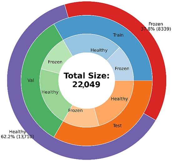
Figure 1.
Proportions of healthy and frozen samples of the dataset of pomegranates.
2.3. Proposed Methods for Image Analysis
The proposed methodology for the identification of frozen pomegranates combines hyperspectral images and detection algorithms using deep neural networks. After obtaining the hyperspectral images, they are analyzed with a neural network model. This network receives each of the spectral images and produces a binary classification, healthy/frozen. For this purpose, we used six different models: ResNeXt, RegNetX, RegNetY, EfficientNetV2, VisionTransformer and SwinTransformer. Each of these networks is trained with the training data, measuring its accuracy on the test set. Their results are compared to determine the best classification methods for the problem of interest. Each of these deep network models is described in detail below.
2.3.1. ResNeXt
Residual Networks (ResNeXt) [27] is a convolutional neural network model based on ResNet. In this model, there are a number of cardinal blocks, each of which contains a number of convolutional layers. In addition, like ResNet, there are hop layers in each path. Finally, the results in the parallel paths are summarized in each cardinal block. The main hyperparameters of this model are cardinal width (number of parallel paths), block depth and bottleneck width.
2.3.2. RegNet (RegNetX and RegNetY)
Regularized Networks (RegNet) [20] attempt to constrain the design space and find the best set of parameters and hyperparameters using regularization techniques. This model, by applying changes to the ResNet network, tries to build more general networks called AnyNetX and AnyNetY, which have multiple hyperparameters. The main difference between AnyNetX and AnyNetY networks is in the way the hyperparameters are searched, so that AnyNetY networks have gone through the fine-tuning process more than AnyNetX and have better results. The training process of RegNet is such that it first considers a large design space and at each stage it trains the models in this space a little (about ten epochs). Then, according to the results of the networks, it limits the design space so that networks with better performance than the threshold should be placed in this new space.
2.3.3. EfficientNetV2
EfficientNetV2 [28] tries to solve the problem of the slowness of the EfficientNet training for large images. This network has used the progressive learning technique. Thus, in the early stages, it resizes the photos to small sizes, and in the later stages, while enlarging their size, it uses regularization techniques such as augmentation to prevent the phenomenon of overfitting. In addition, EffientNetV2 has used the Training-Aware NAS method, which tries to stabilize the training time by choosing the most appropriate architecture while increasing the prediction accuracy.
2.3.4. VisionTransformer
VisionTransformer [29] is a Transformer model that divides the input image into 16 parts (patches) and serially passes them along with additional information (including patch index and overall image class) to the Transformer encoder unit to finally obtain the prediction result. Up to now, Transformer models have generally been used for Natural Language Processing (NLP). In the current model, the whole image and its parts are similar to the sentence and its tokens in natural language, respectively. This model has quadratic spatial complexity due to the division of the image into fixed parts, and its neglect of the locality of the image content makes it less accurate for classifying small datasets.
2.3.5. SwinTransformer
SwinTransformer [30] tries to solve the problems of VisionTransformer. It uses a hierarchical design that first divides the image into four windows and then divides each window into more parts. At each stage, by calculating the self-attention of each part, it finds the parts that have complementary information while being placed in different windows and adjusts the windows accordingly. This process linearizes spatial complexity.
2.4. Evaluation Criteria of the Classifiers
2.4.1. Cross Entropy Loss
The cross-entropy loss function is used to check the loss of the prediction model compared to the actual labels of the inputs. This function calculates the loss for each yi and pi, which are the actual label values and the probability of being labeled as yi by the model, respectively, as indicated in Equation (1) [31].
2.4.2. Confusion Matrix
The confusion matrix is constructed using the original data class and the class predicted by the considered model by determining the number of samples that the model predicted correctly and incorrectly for each positive or negative class. In the confusion matrix, the healthy class is considered positive and the frozen class is considered negative, as shown in Table 1. The number of samples correctly labeled as positive and negative are considered true positive and true negative, respectively. Similarly, the number of samples falsely labeled as positive or negative is called False Positive and False Negative, respectively.

Table 1.
2D confusion matrix for the classification of pomegranate.
2.4.3. Accuracy
Accuracy is the overall correctness of the model prediction and is calculated according to Equation (2) [32].
2.4.4. Precision
Precision is the percentage of correct predictions made by the model out of all its positive predictions and is calculated according to Equation (3) [33].
2.4.5. Recall
Recall is the percentage of positive labels that the model correctly classifies and is calculated according to Equation (4) [32].
2.4.6. F1-Score
F1-Score is a measure to check the trade-off between Precision and Recall and is obtained by calculating the harmonic average of these two values. In other words, a high F1-Score value indicates that the model does not have too many false positive predictions (indicating low Precision) or false negative predictions (indicating low Recall), as presented in Equation (5) [32].
2.4.7. Precision-Recall Curve (PRC)
The PRC curve measures the trade-off between precision and recall by examining different thresholds. In fact, for a low threshold, the probability of getting a positive label for more entries increases. Also, for a high threshold, the probability of getting a negative label for more entries is high. Therefore, a high PRC indicates a good trade-off between precision and recall.
2.4.8. ROC Curve and ROC-AUC
The receiver operating characteristic (ROC) curve examines the trade-off between true positive rate (TPR) and false positive rate (FPR) for different thresholds (Equation (7)). The value of the area under this curve (AUC) measures the model’s balance between TPR and FPR [32].
2.5. Structure and Implementation of the Classifiers
The Adam optimizer was used to load the data with a batch size of 10 and to optimize the process of fitting the models, which has low memory cost and high speed [31]. The cross-entropy loss function was used as the criterion function of the optimizer. The training rate of the models was 0.001, and, in cases where the performance of the model was not suitable, this value was reduced to 0.0001 or 0.00001.
The process of training, validating and testing the models was implemented in the Google Colab environment and with the Tesla T4 GPU. The reason for using this batch size was the memory limitation of this environment. All models were trained for 30 epochs; in each epoch they were measured with validation data and, if they had more accuracy than the previous checkpoint, they were saved as a new checkpoint.
3. Results
3.1. Comparison of Models in Terms of Training Time and Size
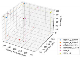
Unlike other models, such as ResNeXt, RegNet models do not have a fixed network size due to the use of the Gradual Channel Growth technique, and during training the number of layers and neurons in each layer changes as needed. As a result, its memory consumption is 3 to 16 times less than other models. On the other hand, due to the fine-tuning of the design space, its accuracy is very high and its training process is about 2 to 3 times faster than other models.
The reason for the insufficient accuracy of the small EfficientNetV2 model is that it requires data for larger models (medium and large). However, these models are much slower than the other models used, and at the same time their size is several times larger than other models, as shown in Table 2.

Table 2.
Comparison of models in terms of training time and size.
3.2. Classification Results of the Classifiers
3.2.1. ResNeXt
The accuracy and loss plots of the ResNeXt model, trained with a training rate of 0.001, are shown in Figure 2. This model reached the highest accuracy value during the 30th epoch in the 23rd epoch. In this epoch, the value of accuracy and loss of the test data is shown with a green dashed line.
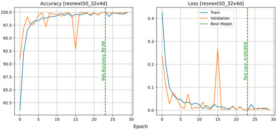
Figure 2.
Accuracy and loss plots of the ResNeXt model.
The confusion matrix of the ResNeXt model is shown in Figure 3. As can be seen, the number of FN is higher than FP, which may be the reason for the class imbalance solution. Therefore, if the negative class data were increased to a smaller number or the threshold was adjusted more compulsively, probably a better fit between the incorrect and correct predictions would be established. Nevertheless, the performance of the model was very good.
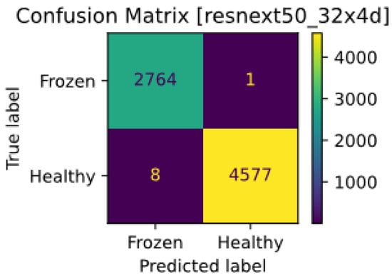
Figure 3.
Confusion matrix of the ResNeXt model.
From the sum of the precision-recall graphs and the ROC-AUC shown in Figure 4, which is 1, it can be concluded that the ResNeXt model is able to maintain a proportional balance between positive and negative class predictions, and the number of false predictions was generally negligible.
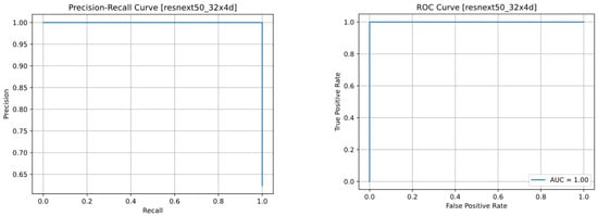
Figure 4.
Precision-recall (left) and receiver operating characteristic (ROC) (right) curves of ResNeXt.
3.2.2. RegNet (RegNetX and RegNetY)
In this article, RegNetX and RegNetY of the same size are used to investigate functional and non-functional differences. Both models are trained with a learning rate of 0.001. The accuracy and loss plots of the RegNetX800MF and RegNetY800MF models are shown in Figure 5. These two models have both been able to fit and reach the accuracy of 99.9% on the test data, with the difference that the RegNetY model reached the best performance earlier. In addition, after the 10th epoch, the fluctuations of the RegNetY model are less, which is due to the difference in the algorithm used during training to find the best design space.
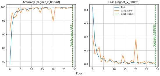
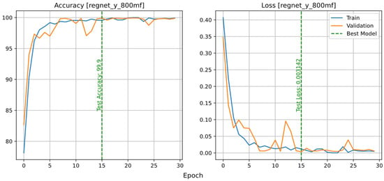
Figure 5.
Accuracy and loss plot of the RegNetX (top row) and RegNetY (bottom row) models.
As mentioned in the previous section, the accuracy of both models was the same on the test data, and as a result, the number of incorrect predictions is the same. The difference is that the RegNetX model has more FN predictions and RegNetY has more FP predictions, as shown in Figure 6.

Figure 6.
Confusion matrices of the RegNetX (left) and RegNetY (right) models.
Considering that both models had high precision and recall, their ROC and Precision-Recall plots are ideal, as shown in Figure 7.
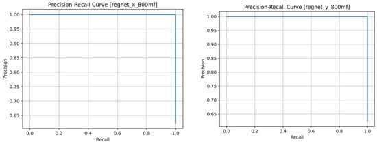
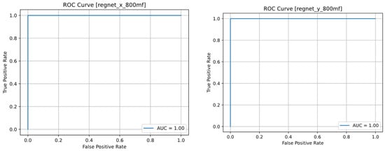
Figure 7.
Precision-recall and ROC curves of the RegNetX (left column) and RegNetY (right column) models.
3.2.3. EfficientNetV2
This network has three different sizes, small, medium and large, as indicated in Table 3. As shown in Figure 8, the small model did not perform well on the test data. On the other hand, according to Table 3, the medium and large models are much slower and larger than the other models. The reason for this is that these models use larger and a greater number of filters, as well as more layers. In addition, the accuracy of the test data of the large model is slightly lower than that of the medium model, which may mean that the medium model is a better fit and there is no need for a model with the complexity of the large model.

Table 3.
Comparison of the proposed classifiers with other methods in the literature for detection of frozen agricultural products.
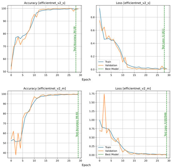
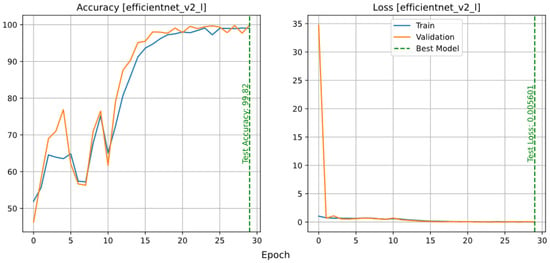
Figure 8.
Accuracy and loss plots of the EfficientNetV2 model in three different sizes: small (top row), medium (middle row), and large (bottom row).
The confusion matrices of the EfficientNetV2 models are shown in Figure 9. As expected, the small model has many errors for both classes, but the medium model has a lower number of incorrect predictions than the other models. The precision-recall and ROC curves of the EfficientNet models are shown in Figure 10. As expected, the curves of the medium and large models are almost vertical and their ROC-AUC is equal to one, which means that the balance between precision and recall is proportional to the number of correct positive and negative predictions. On the other hand, to analyze the Precision-Recall plot and the ROC of the small model, it is necessary to check the effect of different threshold values on Precision, Recall and FPR and TPR ratios (Figure 11). As the threshold increases, the value of Recall or TPR first has a slow downward slope and then a sudden drop for values higher than 0.9, which means that the model has continuous FN predictions. The higher the threshold, the higher the rate of these predictions (this problem can be caused by slow training and can be solved with more training). On the other hand, by examining the changes in Precision and FPR, it can be concluded that increasing the threshold reduces the number of FP predictions of the model, although the rate of these predictions decreases. According to the trend of the first graph, another solution that can be offered to maximize Precision and Recall is to consider the intersection point of these two graphs as the decision probability (for the EfficientNetV2S model it is about 0.32). Trying this solution increased the accuracy of the model from 94.08% to 94.57%.
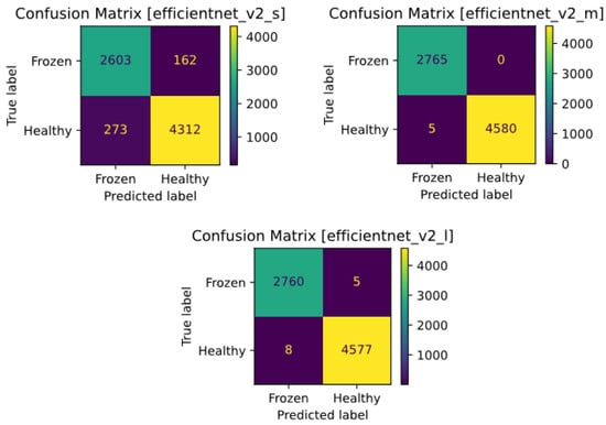
Figure 9.
Confusion matrices of the EfficientNetV2 model with different learning rates: small (top left), medium (top right), and large (bottom row).
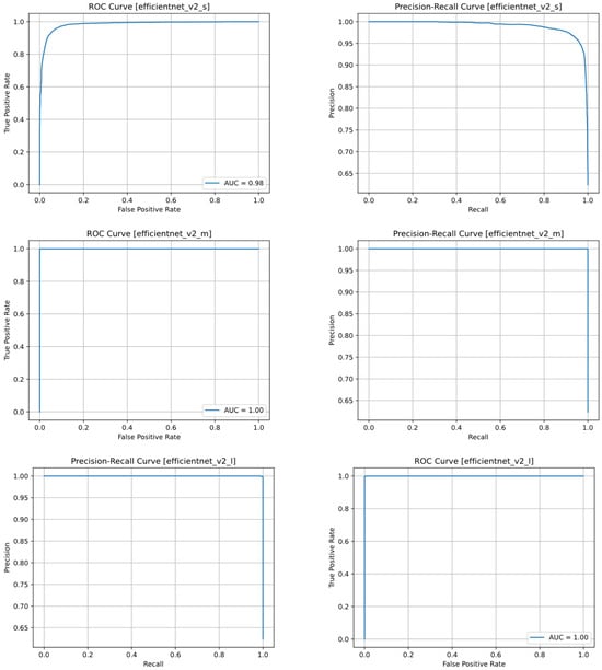
Figure 10.
Precision-recall and ROC curves of the EfficientNetV2 model for 3 different sizes: small (top row), medium (middle row), and large (bottom row).
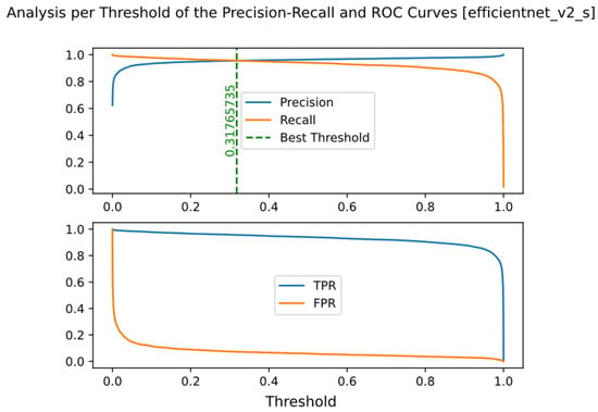
Figure 11.
Investigation of the thresholds on precision and recall (top row), FPR and TPR (bottom row) ratios for the small size of the EfficientNetV2 model.
3.2.4. VisionTransformer
In the case of the VisionTransformer model, the learning rate of 0.001 was not sufficient for it to learn, and only when the learning rate was reduced to 0.00001 did it fit properly. Figure 12 shows that this model could not be fitted with values of 0.001 and 0.0001. At a learning rate of 0.001, it predicted almost randomly; this problem slightly improved using a learning rate of 0.0001, and it was fully solved at a learning rate of 0.00001.
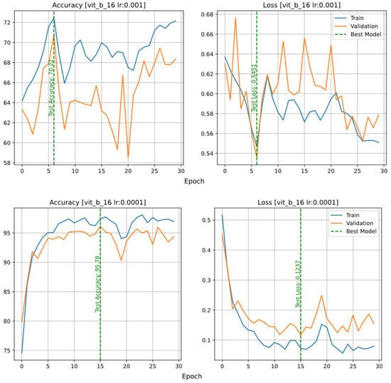
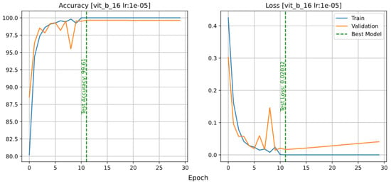
Figure 12.
Accuracy and loss plots of the VisionTransformer model with different learning rates: 0.001 (top row); 0.0001 (middle row); 0.00001 (bottom row).
The confusion matrices of the models with different learning rates are shown in Figure 13. As expected, the model with a learning rate of 0.001 predicted almost randomly, but its performance was more accurate in predicting negative labels. This problem was improved and solved for the models with learning rates of 0.0001 and 0.00001 incrementally.
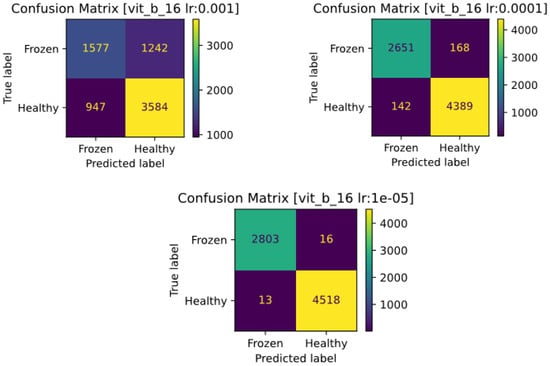
Figure 13.
Confusion matrices of the VisionTransformer model with different learning rates: 0.001 (top left); 0.0001 (top right); 0.00001 (bottom row).
The Precision-Recall and ROC curves of the VisionTransformer model with different learning rates are shown in Figure 14. The appearance of the diagonal ratio of the curves of the model with a learning rate of 0.001 clearly shows the randomness of its selection. In addition, the incremental improvement of the models with learning rates of 0.0001 and 0.00001 can also be seen in Figure 14.
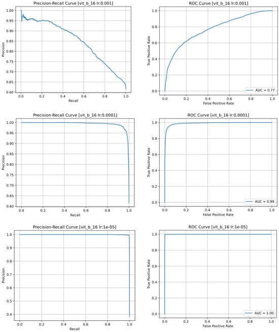
Figure 14.
Precision-recall and ROC curves of the VisionTransformer model for 3 different learning rates: 0.001 (top row); 0.0001 (middle row); 0.00001 (bottom row).
3.2.5. SwinTransformer
As in the previous case, the SwinTransformer model did not fit properly with a learning rate of 0.001, so it also had to be reduced to 0.00001. The accuracy and loss plots are shown in Figure 15. The graph of the models with learning rates of 0.001 and 0.0001 produced completely random output values, but by reducing the learning rate to 0.00001, the model fits correctly.
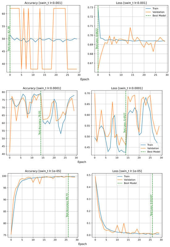
Figure 15.
Accuracy and loss plots of the SwinTransformer model with different learning rates: 0.001 (top row); 0.0001 (middle row); 0.00001 (bottom row).
The confusion matrices of the models with different learning rates are shown in Figure 16. The model with a learning rate of 0.001 is marked with positive data for all inputs. This problem can also explain the successive jumps in the accuracy and loss values of this model. Reducing the learning rate by 0.0001 still has a random output, but its superiority over the first model is that it does not consistently have the same output. Further decreasing the learning rate to 0.00001 makes the model learn more accurately.
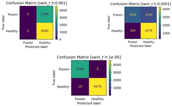
Figure 16.
Confusion matrices of the SwinTransformer model with different learning rates: 0.001 (top row); 0.0001 (middle row); 0.00001 (bottom row).
The Precision-Recall and ROC curves of the SwinTransformer model with different learning rate values are shown in Figure 17. In the graphs related to the learning rate of 0.001, the number of TP and FP labels is high for low thresholds and gradually decreases almost uniformly. The low precision, even when the recall is high, indicates the completely positive predictions of this model. The model with a learning rate of 0.0001 has some correct predictions for small Threshold values, but around 0.1 the number of FNs suddenly increases, and after a while it increases due to the increase in the number of TPs. Finally, by doubling the Threshold value, the number of all model predictions will be FN, and as a result, the Precision will reach zero. In contrast to these models, the third model, trained with a learning rate of 0.00001, fits well and its Precision-Recall and ROC graphs are vertical.
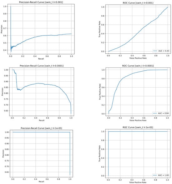
Figure 17.
Precision-recall and ROC curves of the SwinTransformer model for 3 different learning rates: 0.001 (top row); 0.0001 (middle row); 0.00001 (bottom row).
3.3. Comparison of the Classifiers
As a summary of the results presented in the previous subsections, Figure 18 shows the accuracy, precision, recall, and F1 values of all models, namely ResNeXt, RegNetY, RegNetX, EfficientNetV2, VisionTransformer, and SwinTransformer. The accuracy values of the ResNeXt, RegNetX, RegNetY and EfficientNetV2 models are all around 99.9%, and the other two models are probably lower due to lack of data. Clearly, SwinTransformer performs better than VisionTransformer because it considers the interaction (locality) between the windows contained in the image. Among the models, the precision value of the VisionTransformer model is lower, while its recall value is high, which means that it has more FPs and less FNs. In addition, the precision value of RegNetX and EfficientNetV2 models is almost equal to 1, which means that the number of their FPs is 0. In general, due to the higher accuracy value of the EfficientNetV2 model, as well as its relatively high precision and recall compared to other models, the F1 value of this model is also higher than the others.
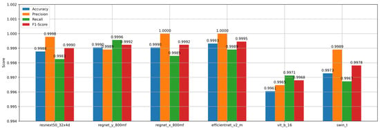
Figure 18.
Comparison of the accuracy (blue), precision (orange), recall (green), and F1 (red) scores for all the studied models.
For completion, some color pictures of the healthy and frozen pomegranates are depicted in Figure 19. Note that these images have been included here only to show what healthy and frozen fruits look like, and that this type of image is not used in the classification models.

Figure 19.
Color pictures of two healthy (left) and frozen (right) pomegranates used in the experiments.
In addition, some sample images of correct and incorrect classifications associated with each of the aforementioned models are shown in Figure 20. Since the EfficientNetV2M and RegNetX models did not produce any false positive image, no figure is available for them.
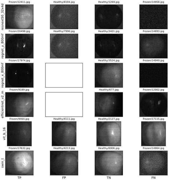
Figure 20.
Some examples of images predicted as true positive (TP), false positive (FP), true negative (TN), and false negative (FN) by each of studied models.
Finally, in Table 3 we can compare the results obtained with the results reported by other authors, which constitute the state of the art in freezing detection in fruits and agricultural products. This comparison has been made using similar research works, but it should be noted that they use different products and different datasets, so the results cannot be directly compared. It can be seen that the results obtained in identifying healthy/frozen pomegranates are very promising. The best state-of-the-art methods can detect frozen products with an accuracy between 90 and 98.86%, which is comparable to the results obtained by our proposal. Thus, convolutional neural networks (CNN), which have demonstrated their good characteristics in many other image analysis problems, are also very effective for the classification of frozen products with hyperspectral images, with a slight advantage for networks that do not use transformers.
The results obtained in this research confirm the statements of Nalepa [34] that current advances in sensor technology have provided new possibilities in multispectral and hyperspectral imaging in various fields including precision agriculture. On the other hand, in another study, Bauriegel et al. [35] concluded that hyperspectral imaging can quickly detect head blight seven days after contamination. This conclusion is very valuable because early detection of pollution is important in maintaining human health. Finally, in order to expand the horizon regarding the use of hyperspectral images, we refer to the research of Grosjean et al. [36], who concluded that hyperspectral imaging offers great opportunities for the analysis of lake sediments with sub-varve size and can be used for marine sediments, tree rings or speleothems.
3.4. Discussion and Model Interpretation Using Integrated Gradients
The focus of the present study is on classification at the level of hyperspectral images, not on the spectral analysis. This is because, in the future, it could be applied to images taken in a field by a remote sensing device with some specific spectral band and analyzed off-site by hybrid machine learning algorithms. Figure 21 shows the interpretation of the different models used using Integrated Gradients [33] for some examples. Using Integrated Gradients, it is possible to understand which parts or pixels of the input images are more important in the final decision of the model. The figures on the left show the samples in the 662 nm spectrum and the figures on the right show the result of Integrated Gradients corresponding to each model.
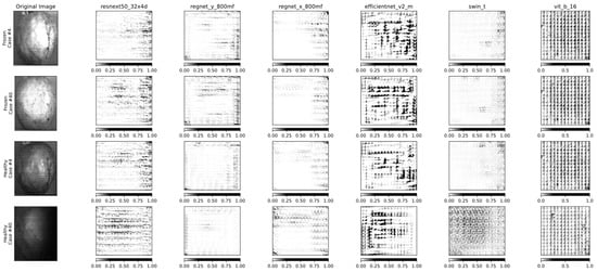
Figure 21.
Different model interpretation using Integrated Gradients [33] for some healthy and frozen pomegranate samples and the 6 deep learning models.
The pixels that contribute most to the final model decision are darker in color. As we can see, the efficientnet_v2_m model is more robust than other models because its decisions are based on different parts of the fruit skin. In addition to the edges and the body of the fruit, this model also pays great attention to the parts of the skin that are more affected by freezing to predict its label and recognize its health. This is a logical decision and interpretation because we see that spots and edges can indicate whether the fruit sample is healthy or frozen.
It is worth mentioning that, in this study, we employed raw grayscale images derived from hyperspectral imaging data to classify healthy versus damaged fruit. This decision was underpinned by our hypothesis that in a comparative analysis between two distinct classes, any inherent noise in the raw data would contribute similarly to both categories. Consequently, we theorized that such noise would be effectively neutralized, minimizing its impact on the relative comparison of these classes. It is important to note, however, that while this approach simplifies the processing pipeline and reduces computational demands, it also bypasses potential benefits offered by calibration techniques, such as removing systematic noise and improving data consistency.
Our findings, within the scope of this study, suggest that the use of raw grayscale images can yield meaningful insights for the classification task at hand. However, we recognize that the incorporation of calibration procedures could further refine our analysis. Such an approach would be particularly relevant in extending our methodology to a broader range of fruits and more diverse conditions, where the nature and magnitude of noise could differ significantly.
Looking ahead, we envisage a comprehensive exploration of calibration techniques in future work. This will not only enhance the robustness of our current model but also expand its applicability and accuracy across various fruit types and conditions. By delving into the nuanced impacts of calibration, our future research aims to establish a more standardized and universally applicable approach in the field of fruit classification using hyperspectral imaging data. This endeavor will contribute significantly to the evolving landscape of agricultural technology and food quality assessment, offering more refined tools for producers and consumers alike.
4. Conclusions
Pomegranates are an agricultural product sensitive to low storage temperatures, which can lead to freezing damage. In many cases, frozen pomegranates cannot be identified by skin color unless they are exposed to ambient temperature for at least 24 h after cold storage. Unfortunately, many fruit fraudsters use colored waxes similar to the color of pomegranate skin to cover the signs of frozen fruits so that they can be easily sold at a high price. In this paper, a method has been developed to identify grenades susceptible to cold damage in a timely and nondestructive manner using hyperspectral imaging. This method would allow for more efficient storage of products, reducing product losses and market value reduction. For this purpose, deep learning neural networks based on ResNeXt, RegNetX, RegNetY, EfficientNetV2, VisionTransformer and SwinTransformer architectures have been used.
The results show that the accuracy values of all proposed models are above 99% with the correct training parameters while the best state-of-the-art methods can detect the frozen products with an accuracy between 90 and 98.86%, which is comparable to the results obtained by our proposal. More specifically, the precision value of RegNetX and EfficientNetV2 models is almost equal to 1, which indicates that the number of their false positive predictions is zero. In general, due to the higher accuracy value of the EfficientNetV2 model, as well as its relatively high precision and recall compared to other models, the F1 score of this model is also higher than the others with a value of 0.9995.
As a future research line, one possibility that has been proposed to improve the accuracy of the small models, such as EfficientNetV2, without sacrificing too much memory is knowledge distillation. It consists in transferring knowledge from a large model to a smaller one, thus maintaining the computational efficiency of the base model. Another possible line of future research is to investigate the wavelengths that are most effective for the detection of frozen fruit. This would allow the construction of specific cameras capable of detecting them using a reduced set of spectral bands.
Author Contributions
Conceptualization, R.P.; methodology, S.S.; software, D.S., M.M.; validation, M.H.R., S.K.; formal analysis, S.S.; investigation, A.M., R.P., S.S., D.S., S.K., G.G.-M., M.M. and M.H.R.; resources, A.M.; data curation, R.P.; writing—original draft preparation, R.P.; writing—review and editing, G.G.-M.; visualization, M.H.R., S.K.; supervision, R.P.; project administration, R.P. and S.S.; funding acquisition, G.G.-M. All authors have read and agreed to the published version of the manuscript.
Funding
This research was funded by project 22130/PI/22 financed by the Region of Murcia (Spain) through the Regional Program for the Promotion of Scientific and Technical Research of Excellence (Action Plan 2022) of the Fundación Séneca-Agencia de Ciencia y Tecnología de la Región de Murcia.
Data Availability Statement
Data is unavailable due to privacy or ethical restrictions.
Conflicts of Interest
The authors declare no conflicts of interest.
References
- Ain, H.B.U.; Tufail, T.; Bashir, S.; Ijaz, N.; Hussain, M.; Ikram, A.; Farooq, M.A.; Saewan, S.A. Nutritional importance and industrial uses of pomegranate peel: A critical review. Food Sci. Nutr. 2023, 11, 2589–2598. [Google Scholar] [CrossRef] [PubMed]
- Maghoumi, M.; Amodio, M.L.; Cisneros-Zevallos, L.; Colelli, G. Prevention of Chilling Injury in Pomegranates Revisited: Pre-and Post-Harvest Factors, Mode of Actions, and Technologies Involved. Foods 2023, 12, 1462. [Google Scholar] [CrossRef] [PubMed]
- Taghipour, L.; Rahemi, M.; Assar, P.; Ramezanian, A.; Mirdehghan, S.H. Alleviating chilling injury in stored pomegranate using a single intermittent warming cycle: Fatty acid and polyamine modifications. Int. J. Food Sci. 2021, 2021, 2931353. [Google Scholar] [CrossRef] [PubMed]
- Ghasemi-Soloklui, A.A.; Gharaghani, A. Determination of freezing tolerance in twenty iranian pomegranate cultivars and its relationship to geographic and climatic distribution and some tree characteristics. Erwerbs-Obstbau 2023, 65, 819–827. [Google Scholar] [CrossRef]
- Malekshahi, G.; ValizadehKaji, B. Effects of postharvest edible coatings to maintain qualitative properties and to extend shelf-life of pomegranate (Punica granatum L.). Int. J. Hortic. Sci. Technol. 2021, 8, 67–80. [Google Scholar]
- Alharbi, A.H.; Alkhalaf, S.; Asiri, Y.; Abdel-Khalek, S.; Mansour, R.F. Automated Fruit Classification using Enhanced Tunicate Swarm Algorithm with Fusion based Deep Learning. Comput. Electr. Eng. 2023, 108, 108657. [Google Scholar] [CrossRef]
- Gill, H.S.; Murugesan, G.; Mehbodniya, A.; Sajja, G.S.; Gupta, G.; Bhatt, A. Fruit type classification using deep learning and feature fusion. Comput. Electron. Agric. 2023, 211, 107990. [Google Scholar] [CrossRef]
- Azgomi, H.; Haredasht, F.R.; Motlagh, M.R.S. Diagnosis of some apple fruit diseases by using image processing and artificial neural network. Food Control 2023, 145, 109484. [Google Scholar] [CrossRef]
- Ditcharoen, S.; Sirisomboon, P.; Saengprachatanarug, K.; Phuphaphud, A.; Rittiron, R.; Terdwongworakul, A.; Malai, C.; Saenphon, C.; Panduangnate, L.; Posom, J. Improving the non-destructive maturity classification model for durian fruit using near-infrared spectroscopy. Artif. Intell. Agric. 2023, 7, 35–43. [Google Scholar] [CrossRef]
- Liao, S.; Wu, Y.; Hu, X.; Weng, S.; Hu, Y.; Zheng, L.; Lei, Y.; Tang, L.; Wang, J.; Wang, H. Detection of apple fruit damages through Raman spectroscopy with cascade forest. Spectrochim. Acta Part A Mol. Biomol. Spectrosc. 2023, 296, 122668. [Google Scholar] [CrossRef]
- Nakajima, S.; Kuroki, S.; Ikehata, A. Selective detection of starch in banana fruit with Raman spectroscopy. Food Chem. 2023, 401, 134166. [Google Scholar] [CrossRef] [PubMed]
- Pourdarbani, R.; Sabzi, S.; Rohban, M.H.; Garcia-Mateos, G.; Paliwal, J.; Molina-Martinez, J.M. Using metaheuristic algorithms to improve the estimation of acidity in Fuji apples using NIR spectroscopy. Ain Shams Eng. J. 2022, 13, 101776. [Google Scholar] [CrossRef]
- Pourdarbani, R.; Sabzi, S.; Kalantari, D.; Paliwal, J.; Benmouna, B.; García-Mateos, G.; Molina-Martínez, J.M. Estimation of different ripening stages of Fuji apples using image processing and spectroscopy based on the majority voting method. Comput. Electron. Agric. 2020, 176, 105643. [Google Scholar] [CrossRef]
- Li, X.; Wei, Y.; Xu, J.; Feng, X.; Wu, F.; Zhou, R.; Jin, J.; Xu, K.; Yu, X.; He, Y. SSC and pH for sweet assessment and maturity classification of harvested cherry fruit based on NIR hyperspectral imaging technology. Postharvest Biol. Technol. 2018, 143, 112–118. [Google Scholar] [CrossRef]
- Yu, T.; Hu, C.; Xie, Y.; Liu, J.; Li, P. Mature pomegranate fruit detection and location combining improved F-PointNet with 3D point cloud clustering in orchard. Comput. Electron. Agric. 2022, 200, 107233. [Google Scholar] [CrossRef]
- Yan-hui, C.; Hui-fang, G.; Sa, W.; Xian-yan, L.; Qing-xia, H.; Zai-hai, J.; Ran, W.; Jin-hui, S.; Jiang-li, S. Comprehensive evaluation of 20 pomegranate (Punica granatum L.) cultivars in China. J. Integr. Agric. 2022, 21, 434–445. [Google Scholar] [CrossRef]
- Zhao, J.; Almodfer, R.; Wu, X.; Wang, X. A dataset of pomegranate growth stages for machine learning-based monitoring and analysis. Data Brief 2023, 50, 109468. [Google Scholar] [CrossRef]
- Alamar, P.D.; Caramês, E.T.; Poppi, R.J.; Pallone, J.A. Quality evaluation of frozen guava and yellow passion fruit pulps by NIR spectroscopy and chemometrics. Food Res. Int. 2016, 85, 209–214. [Google Scholar] [CrossRef]
- Rezaei, P.; Hemmat, A.; Shahpari, N. Detecting sunburn in pomegranates using machine vision. In Proceedings of the Electrical Engineering (ICEE), Iranian Conference, Mashhad, Iran, 8–10 May 2018; pp. 654–658. [Google Scholar]
- Jia, W.; Gao, J.; Xia, W.; Zhao, Y.; Min, H.; Lu, J.-T. A performance evaluation of classic convolutional neural networks for 2D and 3D palmprint and palm vein recognition. Int. J. Autom. Comput. 2021, 18, 18–44. [Google Scholar] [CrossRef]
- Xuan, G.; Gao, C.; Shao, Y.; Wang, X.; Wang, Y.; Wang, K. Maturity determination at harvest and spatial assessment of moisture content in okra using Vis-NIR hyperspectral imaging. Postharvest Biol. Technol. 2021, 180, 111597. [Google Scholar] [CrossRef]
- Gerami, K.; Behfar, H.; Jamshidi, B.; Zomorodi, S. Detection of freezing of Thomson variety orange fruit using Fourier transform-infrared spectroscopy and hyperspectral imaging methods. Innov. Food Technol. 2023, 10, 203–214. [Google Scholar]
- Alimohammadi, F.; Rasekh, M.; Afkari Sayyah, A.H.; Abbaspour-Gilandeh, Y.; Karami, H.; Sharabiani, V.R.; Fioravanti, A.; Gancarz, M.; Findura, P.; Kwaśniewski, D. Hyperspectral imaging coupled with multivariate analysis and artificial intelligence to the classification of maize kernels. Int. Agrophysics 2022, 36, 83–91. [Google Scholar] [CrossRef] [PubMed]
- Yuan, Y.; Wang, C.; Jiang, Z. Proxy-based deep learning framework for spectral–spatial hyperspectral image classification: Efficient and robust. IEEE Trans. Geosci. Remote Sens. 2021, 60, 1–15. [Google Scholar] [CrossRef]
- Xie, T.; Han, W.; Xu, S. YOLO-RS: A More Accurate and Faster Object Detection Method for Remote Sensing Images. Remote Sens. 2023, 15, 3863. [Google Scholar] [CrossRef]
- Lowe, A.; Harrison, N.; French, A.P. Hyperspectral image analysis techniques for the detection and classification of the early onset of plant disease and stress. Plant Methods 2017, 13, 80. [Google Scholar] [CrossRef] [PubMed]
- Xie, S.; Girshick, R.; Dollár, P.; Tu, Z.; He, K. Aggregated residual transformations for deep neural networks. In Proceedings of the IEEE Conference on Computer Vision and Pattern Recognition, Honolulu, HI, USA, 21–26 July 2017; pp. 1492–1500. [Google Scholar]
- Tan, M.; Le, Q. Efficientnetv2: Smaller models and faster training. In Proceedings of the International Conference on Machine Learning, Baltimore, MD, USA, 17–23 July 2021; pp. 10096–10106. [Google Scholar]
- Dosovitskiy, A.; Beyer, L.; Kolesnikov, A.; Weissenborn, D.; Zhai, X.; Unterthiner, T.; Dehghani, M.; Minderer, M.; Heigold, G.; Gelly, S. An image is worth 16x16 words: Transformers for image recognition at scale. arXiv Preprint 2020, arXiv:2010.11929. [Google Scholar]
- Liu, Z.; Lin, Y.; Cao, Y.; Hu, H.; Wei, Y.; Zhang, Z.; Lin, S.; Guo, B. Swin transformer: Hierarchical vision transformer using shifted windows. In Proceedings of the IEEE/CVF International Conference on Computer Vision, Montreal, BC, Canada, 11–17 October 2021; pp. 10012–10022. [Google Scholar]
- Guo, Q.; Wang, C.; Xiao, D.; Huang, Q. A novel multi-label pest image classifier using the modified Swin Transformer and soft binary cross entropy loss. Eng. Appl. Artif. Intell. 2023, 126, 107060. [Google Scholar] [CrossRef]
- Ali, R.; Balamurali, M.; Varamini, P. Deep Learning-Based Artificial Intelligence to Investigate Targeted Nanoparticles’ Uptake in TNBC Cells. Int. J. Mol. Sci. 2022, 23, 16070. [Google Scholar] [CrossRef]
- Pourdarbani, R.; Sabzi, S.; Arribas, J.I. Nondestructive estimation of three apple fruit properties at various ripening levels with optimal Vis-NIR spectral wavelength regression data. Heliyon 2021, 7, e07942. [Google Scholar] [CrossRef]
- Nalepa, J. Recent advances in multi-and hyperspectral image analysis. Sensors 2021, 21, 6002. [Google Scholar] [CrossRef]
- Bauriegel, E.; Giebel, A.; Herppich, W.B. Hyperspectral and chlorophyll fluorescence imaging to analyse the impact of Fusarium culmorum on the photosynthetic integrity of infected wheat ears. Sensors 2011, 11, 3765–3779. [Google Scholar] [CrossRef] [PubMed]
- Grosjean, M.; Amann, B.J.-F.; Butz, C.F.; Rein, B.; Tylmann, W. Hyperspectral imaging: A novel, non-destructive method for investigating sub-annual sediment structures and composition. PAGES News 2014, 22, 10–11. [Google Scholar] [CrossRef]
- Zhang, J.; Dai, L.; Cheng, F. Classification of frozen corn seeds using hyperspectral VIS/NIR reflectance imaging. Molecules 2019, 24, 149. [Google Scholar] [CrossRef] [PubMed]
- Zhi-yong, Z.; Xiang-wei, W.; Yong-ming, C.; Yun-bo, B.; Li, W.; Ping, L. Investigation of Hyperspectral Imaging Technology for Detecting Frozen and Mechanical Damaged Potatoes. Spectrosc. Spectr. Anal. 2019, 39, 3571–3578. [Google Scholar]
- Siedliska, A.; Baranowski, P.; Zubik, M.; Mazurek, W. Detection of pits in fresh and frozen cherries using a hyperspectral system in transmittance mode. J. Food Eng. 2017, 215, 61–71. [Google Scholar] [CrossRef]
Disclaimer/Publisher’s Note: The statements, opinions and data contained in all publications are solely those of the individual author(s) and contributor(s) and not of MDPI and/or the editor(s). MDPI and/or the editor(s) disclaim responsibility for any injury to people or property resulting from any ideas, methods, instructions or products referred to in the content. |
© 2024 by the authors. Licensee MDPI, Basel, Switzerland. This article is an open access article distributed under the terms and conditions of the Creative Commons Attribution (CC BY) license (https://creativecommons.org/licenses/by/4.0/).
