Article

Using Entropy Metrics to Analyze Information Processing Within Production Systems: The Role of Organizational Constraints

by
Frits van Merode
1,2,*,
Henri Boersma
1,3,
Fleur Tournois
4,
Windi Winasti
5,
Nelson Aloysio Reis de Almeida Passos
6,7 and
Annelies van der Ham
1,8
1
Care and Public Health Research Institute (CAPHRI), Maastricht University, 6200 MD Maastricht, The Netherlands
2
Maastricht University Medical Centre+, 6229 HX Maastricht, The Netherlands
3
Department of Radiology & Nuclear Medicine, Maastricht University Medical Centre+, 6229 HX Maastricht, The Netherlands
4
Department of Gynecology and Obstetrics, Maastricht University Medical Centre+, Maastricht University, 6229 HX Maastricht, The Netherlands
5
Elisabeth-TweeSteden Ziekenhuis, 5022 GC Tilburg, The Netherlands
6
Department of Computer Science, University of Pisa, 56126 Pisa, Italy
7
Institute of Information Science and Technologies, National Research Council, 56124 Pisa, Italy
8
Rhythm, 1014 AX Amsterdam, The Netherlands
*
Author to whom correspondence should be addressed.
Logistics 2025, 9(2), 46; https://doi.org/10.3390/logistics9020046
Submission received: 9 January 2025 / Revised: 12 March 2025 / Accepted: 19 March 2025 / Published: 26 March 2025

Abstract

:
Background: The literature on measuring the complexity of production systems employs the graph and information theory. This study analyzes these systems and their coordination under varying states of control, with a focus on the probability of unfavorable events and their temporal characteristics. Methods: Coordination systems are represented as temporal networks, using entropy and node influence metrics. Two case studies are presented: a factory operating under the principles of the Toyota Production System (TPS) with adjacent (local) coordination and andon (global) coordination and a university obstetrics clinic with only adjacent (local) coordination. Results: Adjacent coordination leads to zero entropy in 38.40% of all situations in the TPS example, contrasted to 76.62% in the same system with andon coordination. Degree centrality of nodes outside of zero-entropy situations exhibits higher average and maximum values in andon coordination networks, compared to those with adjacent coordination in TPS. Entropy values in the university obstetric clinic range from 0.92 to 2.23, average degrees vary between 3 and 4.08, and maximum degrees range from 7 to 9. Conclusions: Coordination systems modeled as temporal networks capture the evolving nature of centralizing and decentralizing coordination in production systems.

1. Introduction

Research on assessing the complexity of production systems, including supply chain systems, using entropy measures has been ongoing since the 1980s. A key metric in this field is graph entropy, which quantifies the information processing structure of a production system and serves as an “effective measure of complexity” [1]. In this context, complexity can be attributed to the physical network of factories, distribution centers, warehouses, and outlets—referred to as nodes—connected through links that represent movements and transport—referred to as edges. In modern, highly integrated supply chain networks, such as multi-stage assembly systems and multi-echelon supply chains, entropy measures are essential for describing complexity propagation [2]. For instance, in mixed-model assembly systems, manufacturing complexity significantly influences complexity propagation, making the consideration of “system configuration, task-to-station assignment, and assembly sequences” essential for their analysis [1].
As manufacturing and supply chains become increasingly integrated, they are hereby collectively referred to as “production systems”. Assessing the probability that a production system remains in control, despite uncertainties in its coordination mechanisms, is crucial [3]. To achieve this, the coordination system must possess requisite variety to adapt to environmental changes. Furthermore, when disruptions occur, the production system must exhibit resilience to restore its original state [4,5,6,7,8]. When a production system is modeled as a network, the nodes represent locations where products are manufactured, stored, or sold, while the edges signify movements, such as transportation, between these nodes. In this context it does not fully capture the complexity of a supply chain network by itself, even though Shannon entropy serves as a robust measure of the structural properties of the physical network. Additional metrics, such as the number of edges and the distance between nodes, are often employed to provide a more comprehensive analysis. Certain nodes may be critical to the supply chain’s functionality, thereby requiring a thorough evaluation of their complexity, encompassing node influence metrics and the uncertainty associated with their activation, to ensure a comprehensive understanding of their role within the supply chain. Measuring the entropy of the coordination network is proposed here as a complementary metric to the existing measures of the physical structure’s complexity and stability.
A crucial distinction must be made between the coordination network and the physical network that it manages: the former can be understood as a set of constraints imposed on the latter. Note that although the two production systems may exhibit identical Shannon entropy values for their physical networks, they might differ significantly in the entropy of their coordination systems. The problem statement therefore is: How can Shannon entropy be calculated and utilized to measure the complexity of coordination in production systems? To answer this, a methodology for calculating the Shannon entropy of coordination networks is introduced and illustrated by two contrasting examples: a factory operating under the Toyota Production System (TPS) principles, characterized by low levels of uncertainty due to optimization, and an obstetrics clinic, which operates with high levels of uncertainty, necessitating a more flexible and complex coordination system. These two systems were selected for their contrasting characteristics, as these are expected to have a profound impact on their quantified entropy and additional complexity metrics. The obstetrics clinic is subject to three key types of uncertainties that are either absent or noticeably different in TPS: (1) in the clinic new patients arrive unpredictably, in contrast to TPS, where the arrival of orders at workstations is carefully planned; (2) the procedures required for admitted patients are not known in advance in the clinic, whereas in TPS, the processes for handling orders are well-defined; and (3) the length of stay for admitted patients varies, even when the procedure is known, while in TPS, order processing times are standardized or nearly precisely estimated. These differences highlight the varying coordination demands and complexities inherent in the two systems.
The two systems are analyzed through the lens of how constraints related to the coordination network influence the reduction in coordination complexity and the entropy of production systems. Both systems are modeled as graphs, and the effects of these constraints are evaluated by measuring the resulting complexity reduction. Notably, the entropy values of coordination networks can even differ among otherwise identical factories and production systems. Such variations may be intentional, because of deliberate design choices, or unintentional, occurring when the system operates beyond its designed parameters (i.e., in an open-loop state). By studying the constraints imposed on coordination networks, distinctions between entropies stemming from intentional design and those arising from out-of-control conditions can be made. The proposed method analyzes the structure of coordination networks only, therefore dismissing any additional information on their contents. Table 1 provides an overview of the study and the present article.

2. Coordination and Network Entropy

The contrasting examples studied can be placed in a typology of coordination systems, as presented in Appendix A. The university obstetric clinic is characterized by the absence of feedback loops: workflows from upstream to downstream, independently of the status of the latter, corresponding to coordination system type (a) in Appendix A. In contrast, Toyota Production Systems operate with both local and global feedback loops, which facilitate release and work-in-progress coordination. These correspond with coordination system types (f) and (g) in the typology presented in Appendix A. In systems with multiple production lines, a synchronization of release and work-in-progress occurs (coordination type (g) of the typology in Appendix A).
A coordination system can be viewed as the outcome of arbitrary communication [9], as cited by [10], and may be appropriately represented as a network. A network is mathematically described as a graph consisting of nodes (vertices) and edges (links), where an edge connects two nodes if they are related by a specific criterion [11]. Shannon’s entropy formulas can then be applied to quantify the information content within the coordination system. Since the mid-1980s, entropy measures have been used to analyze production systems, initially focusing on the flexibility of manufacturing systems. The first study on flexibility in this context, to the best of available knowledge, was conducted by Vinod Kumar [12]. The application of entropy measures to analyze the complexity and information-processing capacity of supply networks emerged later, with an early example being the work of Battini et al. [13], followed by numerous subsequent studies. The COVID-19 pandemic has recently drawn renewed attention to the risks of supply chain disruption, prompting studies to assess the complexity of supply chains using entropy measures [8] and optimize production system resilience [5], e.g., by determining their optimal amount of redundancy [7].
Over time, the fields of manufacturing and supply chain management have become increasingly integrated, particularly in industries where supply chains are tightly coupled with just-in-time manufacturing processes. In this context, graph entropy metrics have gained attention, due to their ability to distinguish between different types of networks from a structural perspective [14], i.e., by analyzing both individual nodes and the overall network’s structural properties. To fully quantify the entropy of a production system, it is essential to describe both aspects, as greater diversity among the nodes increases the amount of information required to describe the network [15]. This diversity can be captured, for example, by the nodes’ degrees, i.e., the sum of incoming and outgoing edges for each node in a directed graph.
A coordination system, therefore, arises from the network properties of the production system, combined with the emerging constraints on the set of possible coordination networks. Morzy argues that entropy metrics should reflect the properties of this generative process [16], or the effective complexity, as defined in the algorithmic information theory by Gregory Chaitin [17]. The effective complexity is quantified by the length of the most concise description of a system [18] (p. 228), [19]. The representation of a network also depends on its level of coarse-graining and aggregation, which can be arbitrary [16]. This implies that, when comparing various production systems, coordination networks must be generated with consistent coarse graining applied throughout. The process structure of a production or service network, along with the constraints that govern its possible states, can be viewed as a program (in the sense of algorithmic information theory) that generates a coordination network. Algorithmic complexity is low when the entropy of the coordination network is low. Conversely, when entropy is high, the algorithmic complexity can be either high or low. As Zenil et al. [20] note, high entropy may overestimate the randomness of a system, while low entropy may underestimate the randomness at the node level, and consequently, the overall randomness of the system. This suggests that in a coordination system with low entropy, certain nodes may become overloaded.
A recent overview of the use of entropy regarding production systems [21] shows that especially the Shannon entropy has been used to measure the complexity of production systems, due to its simplicity, generality, and strong theoretical foundations. Other entropy measures, such as an analogy of Boltzmann–Gibbs, are sometimes used as well. A distinction should be made in what is exactly measured, as these measures emphasize distinct aspects of complexity [21]. Shannon entropy measures information uncertainty and diversity in a system [22]. The focus is on task assignments and workflow changes, such as the diversity of product types or process variations. Boltzmann–Gibbs entropy originates from statistical mechanics and measures the number of microstates corresponding to a macrostate [22]. The focus is on the number of ways that the tasks/resources can be set up to establish a stable system. Considering the above, Shannon entropy is used in this study.
When analyzing the coordination complexity of production systems, Shannon entropy is frequently applied to quantify task unpredictability and coordination diversity. The total complexity of the production system is determined by the complexity of its structure (including the capability to deal with product variants) and the complexity which results from process uncertainty [23]. The measures of both types of complexity together lack consistency [23]. This problem is related to what Martignago et al. observe in their overview of research and applications of entropy measurement in supply networks. They observe that indexes (i.e., entropy measures) found in the literature compare alternative graphs and do not have much value when only a single graph is considered [21].

3. Graph Theory to Describe Network and Situation Entropy

3.1. Shannon Entropy

The states of production and service systems change constantly due to internal and external inputs. Managing these changes, whether desired or undesired, is at the core of coordination. This study focuses on the application of Shannon entropy [24], in which the uncertainty of outcomes is represented by a discrete random variable X . Shannon’s information entropy for n possible outcomes, with n outcomes ( x 1 , x 2 , x n ), can be calculated by Equation (1):
H X = i = 1 n P x i l o g 2 P x i
The information available in such a system, e.g., a supply chain, can be measured by probability distribution, and Shannon’s network entropy can be used to assess its complexity. To calculate it, the similarity between the node degrees in a graph is often used [15,25], leading to Equation (2):
H g r a p h = i = 1 n d e g v i m l o g 2 d e g v i m
where n is the number of nodes, m the number of edges, and d e g v i is the number of edges incident to node v i [25]. This definition of graph entropy will be used consistently throughout the study, unless otherwise specified, when the term ’entropy’ is used.

3.2. The Complexity of Coordination

To analyze the complexity of coordinating production systems, the following types of complexity are distinguished: design complexity, coordination complexity, and node complexity.

3.2.1. Design Complexity

Design complexity refers to the complexity involved in designing the coordination system. Before a production system can operate, it must first be designed. This can be a single-step process, but in most cases, it is a gradual development which may span several years. For example, building a physical factory may occur within a specific period, but developing operating systems that are effective and adaptable to changing circumstances can take much longer. The network of suppliers and customer channels can be even more intricate. Changing circumstances, along with continuous improvement efforts, aim to make the production system as effective and efficient as possible. To synchronize the flow of products and materials within the factory and across the entire supply chain, cycle times for all production phases should ideally be equal [26] (p. 348). This standard cycle time, which coordinates the whole production system and under which systems strive to operate, is called “Takttime”. However, achieving perfect equality across all cycle times without slack capacity is impossible due to inevitable disruptions in production. The design challenge is to minimize the probability that delays at one location—whether at a workstation or across the supply chain—will disrupt the entire system. The optimization task is to set the Takttime as low as possible while accepting the following conditions:
  • Extra coordination is needed when Takttime cannot be met at a specific moment or location in the production system.
  • Both additional capacity and coordination are required when Takttime is exceeded.
A fundamental concept of the Toyota Production System (TPS) is shortening the supply chain [27] (p. 203). In TPS, manufacturing systems and the supply chain have become highly integrated into a cohesive production system. Toyota (and other companies adopting TPS) expects their suppliers to adopt similar methods [27]( (p. 198). This integration is possible only when the main company has enough power to influence and control its suppliers. In TPS, workers in main factories are also required to be multiskilled. This flexibility enables workers to assist at different workstations, thus “keeping the flow” [28,29]. There can be many sources of disruptions [30]. For the scope of this study the distinction between internal and external sources is important. The design of production systems aims to convert uncontrollable factors into controllable ones. Sharma et al. [31] distinguish between internal and external factors. Variation in process times due to differences in workers’ skill levels is an internal factor that needs to be minimized to meet Takttime. However, if this variation is caused by external factors, such as the supply of raw materials from vendors who are not directly controlled by the production system, then it becomes an uncontrollable external factor. To work within Takttime, the supply of these materials should be internalized within the production system, and the key question becomes to what extent can external factors be made internal. Notably, full control over all factors is not attainable due to uncontrollable events, e.g., the COVID-19 pandemic resulting in supply chain disruptions. This study focuses on the coordination of internal factors.

3.2.2. Coordination Complexity

The complexity involved in coordination is related to the probability of situations occurring with certain levels of entropy. In a production system where cycle times align with Takttime, coordination is simplified and only required at the lowest tiers, as workers can maintain Takttime through routine tasks. The system is therefore designed to accommodate variability and uncertainty, resulting in a lower probability of requiring additional coordination, which stems from high process standardization, minimal errors, and/or slack capacity.

3.2.3. Node Complexity

While the complexity and entropy of the overall network may provide insight into the general challenges within a production system, as discussed in Section 2, it does not reflect the information-processing requirements of its individual agents. Therefore, it becomes crucial to also assess node complexity, which provides a simple yet effective means of evaluating the role of nodes and their influence on the coordination process. Distinct node influence metrics, such as degree centrality, may be employed to capture the extent to which individual agents are dependent on or central to the overall resource and flow within the network. As high-degree nodes are typically more critical to coordination, but face higher operational demands, this simple metric helps to identify potential bottlenecks and vulnerabilities in the system, potentially highlighting areas where additional coordination or resources may be required to maintain its efficiency.
It is assumed that a maximum of one edge can exist between the same pair of nodes at any given moment. Table 2 describes the variables used to describe coordination networks of different production systems.

3.3. Network Simulation

System modeling and analysis simulations were implemented in Python [32], using the following additional libraries: Pandas [33,34]; Matplotlib [35,36]; Plotly [37,38]; NumPy [39]; NetworkX [40,41]; and NetworkX-Temporal [42].

4. Two Examples of Coordination Systems

Two distinct production systems are described: the first is based on the principles of the Toyota Production System (TPS), and the second is a university obstetrics clinic. The TPS case was chosen to introduce key coordination concepts to the present study, which are subsequently applied to analyze both cases, facilitating a comparative examination of their coordination mechanisms.

4.1. Toyota Production System

In the TPS, constant synchronization occurs between the flows moving through the production system. A key characteristic of these systems is the constant time interval (λ), which defines the time between products in the production sequence. This interval, known as Takttime, remains constant in traditional TPS [43] (p. 183), [44]. However, variations in the TPS exist in which the Takttime may vary, depending on factors such as required product features [45,46], demand volume, and patterns [47,48,49].

4.1.1. Slack and Constraints by Design to Deal with Variations

Not all products have the same processing rates within the departments in the TPS. Variation in processing times may occur due to differences in the features ordered by the customer, as well as quality issues with products or parts that need to be addressed within these departments. The throughput time of each product at each department s i consists of three components:
  • pi: Processing time for the product with standard features at the department.
  • pf,i: Extra processing time due to specific product feature requirements at the department.
  • pq,i: Extra processing time of the product due to quality problems at the department.
In a Takttime system, the time intervals λ are determined by design and must be maintained during operational periods, except when the system is disrupted. Boundaries between departments in the production line must be set so that λ remains constant, meaning that for each department s i , the sum of the throughput times p i + p f , i + p q , i must remain balanced. The required amount of slack time is determined during the design phase to handle variations in processing times and quality issues so that this balance is achievable. The selection of features therefore plays an additional, but key role in this stage, as they influence processing times.
The variation in processing times for different features impacts the decision regarding the necessary redundancy in feature production. To minimize this variation, constraints on the number and/or combination of features must be designed. These constraints might limit the choices available to customers, but can be beneficial as well. For example, by grouping certain features together, customers may receive additional features at a lower price, compared to a system where a broad range of specific features can be individually ordered. This approach helps standardize the production process and, in turn, reduces the need for excess slack capacity.

4.1.2. A Closed-Loop Control System

A TPS resembles the coordination networks (f) and (g) described in Appendix A. A key characteristic of these systems is that they are controlled by closed-loops. In the context of system blocks, this control is achieved by design through specifically defined parameters. Slack capacity functions as a buffer at two levels: at the workstation level it accommodates variations in processing time, and at the system level, it ensures a smooth flow by absorbing fluctuations across the production process. Each workstation has a defined trigger time, which indicates when additional help from other workers within the same department is needed to complete the task before the trigger time expires. If there is no time left—or if it becomes apparent that there will not be enough time to finish the task—the ‘andon line’ is pulled, halting the entire production line. This action prompts the allocation of resources from other workstations and preventing new orders from entering the production line. In this system, the status is continuously monitored to ensure full awareness of the production flow. For example, in a one-piece flow system, e.g., where only one car is processed at each station on the production line at given moment, cars are spaced a certain distance apart, which impacts the buffer time at each workstation.

4.1.3. Complexity in a Coordination Network: At System and at Node Level

To assess the complexity of the TPS, it must be analyzed both at the system (global) level and at the workstation (node) level. In the TPS one-piece-flow system, local coordination occurs when the situation reaches a critical point (‘orange’), indicating a higher risk for delays or deviations in the manufacturing process. In this case, one or more operators from neighboring workstations will assist if possible, meaning there is information processing at the local level.
It is also possible that certain orders consistently require assistance from neighboring workstations. This dynamic leads to a series of coordination networks over time, which can be modeled as temporal networks. A temporal network can be represented as a series of snapshots at different times [50], i.e., a list of graphs corresponding to the aggregated dynamics observed in a specific interval. As the overall structure is therefore shaped by “switching moments” [51]—points in time where the network’s configuration changes—temporal graphs are useful to help identify patterns of coordination and relate them to specific switching events. The local entropies in the TPS are always temporary: the probabilities of these events occurring, as well as their durations, are known and determine how much the local entropies contribute to the total system entropy. Balancing the TPS factory involves optimizing the amount of slack capacity in relation to the maximum possible entropy of the coordination system. Several examples of switching events are typical for the TPS, which together illustrate its core principles and the coordination load it imposes. The production system for all examples discussed here is kept fixed: seven workstations are used for two parallel manufacturing processes, and the final product is delivered by workstation 7, as shown in Figure 1.

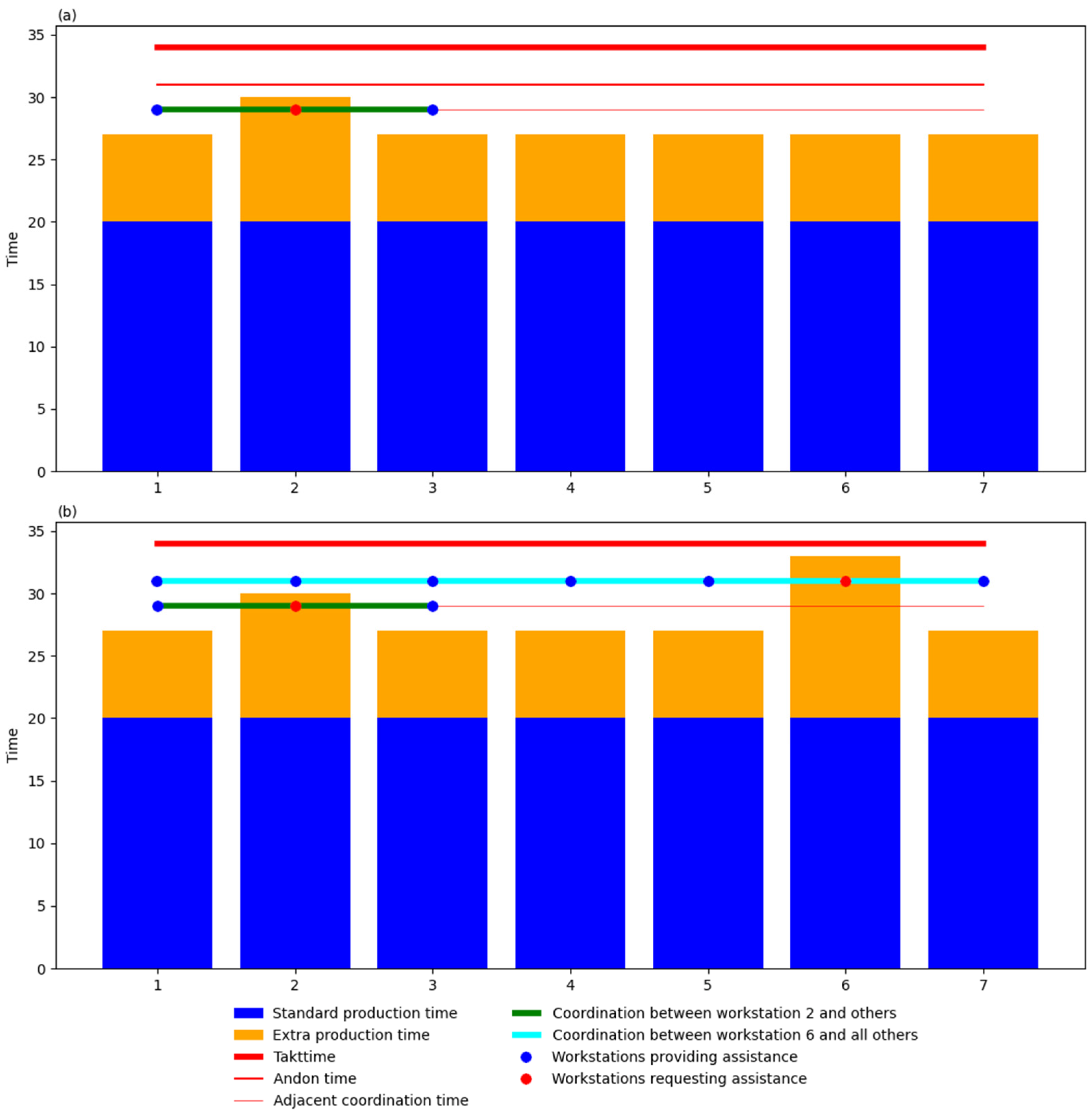
4.1.4. Takttime, Adjacent, and Andon Coordination

The Takttime is always set to be equal to or greater than the required and actual production time at the workstation level. A common cause of variation in production time is the variability in production specifications. For example, in a car factory, the same car model may come with different options; additionally, quality problems might arise, which workers are expected to address at their respective workstations. If slack time were allowed, there would be no need for coordination between workstations. However, this approach is inefficient, and since the effects of product variety or quality problems cannot be fully predicted, a system is employed where the workers at adjacent workstations provide assistance when needed. To manage this, a threshold value is set. For simplicity, only discrete time units (in minutes) are used. As an example, suppose that the Takttime is 34 min and the threshold value is 29 min. The base model requires 20 min, but on average, an additional 7 min is needed to account for product variety and quality issues. Following the approach of [52], the entropy of production time can be calculated as follows: each minute beyond the average cycle time is considered an unfavorable event. The probability p of encountering an unfavorable event i is given by Equation (3):
p i = Δ t d m a x d a v g
where Δ t is the interval between the average duration t a v g and the maximum durations t m a x and the denominator is the range of processing times (in minutes) that exceed the average. The formula captures the probability of a deviation from the average cycle time within this range. Therefore, I = { d a v g + 1 , , d m a x } represents the set of I of all unfavorable events, and the total number of unfavorable events for an activity is equal to the number of elements in the interval d a v g , d m a x . The entropy for the time longer than the average duration is then obtained by Equation (4):
s i = i I i ( d m a x d a v g ) l n ( p i )
Using this duration entropy, a scale is established with two threshold values: (1) help needed from adjacent workstations, and (2) help needed from all workstations in the same factory. In this model, a uniform distribution of duration entropy is assumed. However, as discussed in [52], the same reasoning can be applied using other probability distributions. The trigger value α for requesting help from adjacent workstations is set at a certain threshold, which is defined as α = d m a x 2 . When unfavorable events occur, leading to coordination issues, they can be analyzed using temporal networks. In the TPS, there are two types of trigger values:
  • Help time: time when adjacent workstations are asked (and expected) to provide assistance.
  • Andon time: time when all workstations are asked (and expected) to provide assistance.
Coordination resulting from andon time always has precedence over the coordination prompted by help time. In Figure 2, a time slice is presented where at workstation 2, the trigger value (help time) for adjacent coordination has been reached, while all other workstations are below this threshold; for simplicity this is set at d a v g . Help time is set to 29 min, while andon time is set to 31 min, resulting in a slack time of 3 min in the andon time window to prevent production system disruptions; therefore, highlighting the importance of system design. When selecting the thresholds for help time and andon time, constraints are imposed on the coordination approach. This capacity redundancy, which allows for extra time for processing, is only feasible if the additional work can be completed within the allotted extra time. Specifically, if the operators from adjacent workstations consistently require more than two minutes to provide assistance to other workstations, the help time window should be adjusted upwards accordingly. In the given example, it is therefore assumed that tasks performed by operators from adjacent workstations take less than two minutes. This includes the signaling of the request for help and the duration of their movement. The same reasoning applies to andon time, although its window is often longer to accommodate a wider range of tasks that can be performed by operators from other workstations, providing greater flexibility in responding to support requests. The scope of cooperation, and consequently its coordination, is influenced by factors such as task size, layout (including form and distances), and the possession of multiple skills by the operators. A smaller time window restricts coordination possibilities, while also constraining complexity. In contrast, a larger time window enables greater cooperation, but its coordination may become more intricate. These dynamics are explored in the two examples presented.
By setting help time and andon time as in Figure 2, three coordination zones can be distinguished:
  • Below 29 min: no coordination between workstations is needed.
  • Between 29 and 31 min: coordination occurs between adjacent workstations.
  • Above 31 min: coordination is required from all workstations.
Coordination becomes necessary because workers from workstations 1 and 3 not only need to assist workstation 2, but also because helping others may impact the processing times at their own workstations. In graph theory terms, this system can be modeled with workstations (nodes) and coordination actions as edges. Each edge has a time attribute corresponding to the amount of time allocated for coordination between the workstations. For instance, if the network in Figure 2b is considered as a static graph, the entropy of the entire coordination taking place equals 1.84. Note that in this scenario, workstations belonging to different production lines (e.g., workstations 6 and 3) also require coordination. However, considering the system as a temporal network, coordination activities take place in two time zones, resulting in graph entropies of 0.92 and 0.59, meaning lower coordination efforts. Figure 3 displays a comparison among all representations, considering the network as static or temporal graphs.
When two coordination networks are closely connected and share common nodes, they can be treated as a single, unified network. For the participants, coordination requires time and effort which may add stress to their workload. Therefore, coordination networks operating within the same time zone and sharing nodes are considered as one integrated network. For example, in the static graph scenario, if workstations 1 and 3 also require assistance from adjacent workstations, the following connections occur:
  • For workstation 1, workstation 2 becomes involved.
  • For workstation 3, both workstations 1 and 2 become involved.
This integration allows us to analyze the structural characteristics of coordination networks based on parameters such as help time, andon time, and Takttime. These networks may be categorized into:
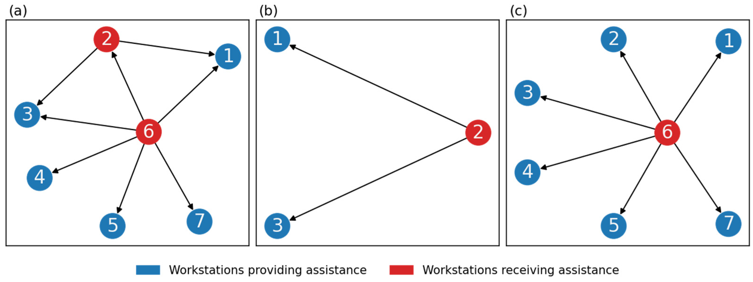
  • Situation networks: formed in response to routine coordination demands based on help time.
  • Andon networks: formed when andon time is reached, requiring broader coordination.
It is important to note that although such networks can be integrated by sharing nodes, they may also remain separate, depending on the situation. Consequently, the analysis must not only measure the entropy of these networks, but also consider other structural metrics, such as the node degrees and number of edges occurring in time zones. Finally, the focus of this study is on coordination networks when the production system is under control, i.e., when Takttime is not exceeded. Networks in which Takttime is exceeded, and the system is effectively out of control, are out of the scope of analysis.

4.1.5. TPS Case Study

This section presents a simulation-based study of a production system based on Toyota Production System (TPS) principles. The study examines scenarios across various time zones, aiming to provide insights into the likelihood of formation of situation networks and andon networks, as well as their structural characteristics. The simulation investigates both the probabilities of process times that lead to the formation of coordination networks and the threshold for network development, i.e., that trigger the creation of situation and andon networks and aims to understand how these factors influence the evolution and complexity of coordination networks under a controlled production system. This enables the identification of patterns and structural properties, such as entropy, node degrees, and edge dynamics in coordination networks, and the analysis of how design choices, such as help time and andon time thresholds, affect the system’s efficiency and ability to manage coordination demands, while maintaining control within the production system.

Scenario Generator

In this scenario, a generator simulates coordination dynamics in a production system with workstations 1 through 7 over a time scale of 1 to 100 time units. The simulation is based on a Monte Carlo process and explores different configurations of parameters, described in Table 3, to study the conditions under which the situation networks and andon networks emerge.
Each scenario is a unique experimental combination of the mean extra time (c2), help time (c3), and andon time (c4). Each Takttime period is simulated n = 1000 times using a Monte Carlo process, and the variations between scenarios are reduced by using a set of n random numbers for the simulations. This approach enables a detailed analysis of how varying mean extra time, help time, and andon time thresholds influence the emergence and complexity of coordination networks within the production system.

Simulation Results

Different scenarios can be identified based on Table 3.
  • No situation or andon entropy (entropy is 0 for both). Occurs when help time, andon time, and maximum duration are identical. Assumes 100% standard process times with no disturbances; in practice, any disturbance would immediately cause the system to fall out of control, as no buffer for coordination exists. This is a highly unrealistic scenario, unless there are no variations in process or task times.
  • Situation entropy exists and there is no chance that andon entropy exists. This is only the case when the andon time is set at the maximum duration time. All process time variations are managed locally through help time coordination. Coordination efforts likely result in situation entropy and an increase in local edges. This set up may be deliberate, such as when an organization prioritizes local coordination or lacks sufficient multiskilled workers for broader (andon) coordination. Without multiskill training, andon coordination is infeasible, and local solutions become the default. Alternatively, this way of coordination may also be a matter of choice, such as in organizations where local over andon coordination may be preferred.
  • Situation entropy exists and there is a chance that andon entropy develops. It is characterized by the maximum process time exceeding andon time. When the maximum possible process time is above andon time, there is always a chance that andon coordination is activated. The likelihood of andon coordination and its entropy therefore increases with longer andon time zones and decrease with longer help time zones—the latter of which reduces the frequency and impact of andon coordination. The interplay between help time and andon time zones determines the balance between localized (situation) and global (andon) coordination efforts.
The amount of entropy and the differences between help time and andon coordination are analyzed by rescaling andon entropies between 0 and 1 and comparing the number of edges. In all 24,000 occurring instantiations, the number of edges and the entropy metrics of the different phases are presented in Table 4 and Table 5. Relative to their entropy values, andon coordination networks have far more edges compared to situation (adjacent) coordination networks when activated, which indicates that the latter are smaller, but less structured, resulting from the merging of local networks—often due to adjacent workstations assisting each other. Although local coordination (help time) appears simple, it gives rise to intricate, dynamic networks as multiple local interactions merge and more complex coordination networks emerge.
The design of help time and andon time thresholds has a significant impact on the coordination load and network complexity. The distinction between help time and andon coordination lies in their scale and structure, where help time manages local disruptions through a simpler, yet less effective approach to address broader issues, and andon coordination addresses larger-scale disruptions, exhibits greater complexity, and requires higher worker skill levels. These findings underscore the importance of striking a balance between slack capacity, training multiskilled workers, and designing optimal thresholds to enhance coordination efficiency.

4.1.6. Phase Transitions and Complexity

A key characteristic of the TPS lies in the deliberate design of phase transitions that guide the system through different states of coordination. These transitions can be described in terms of entropy and node complexity within the coordination networks:
  • From “Need Help” to “Andon”. Triggered by breaching help time threshold, prompting localized coordination. Node complexity increases and entropy rises as local coordination networks emerge, particularly for nodes requiring assistance and their adjacent nodes.
  • From “Andon” to “Out of Control”. Andon time threshold is surpassed, leading to system-wide coordination or failure. Node complexity becomes concentrated, as certain nodes bear disproportionately high coordination loads. Fluctuation of entropy levels is initially high during widespread coordination, then stabilizes at medium levels if resolved efficiently. Otherwise, it peaks at very high levels if the system is overwhelmed (out of control).
The relationship between system-level complexity and the information processing challenges faced by individual agents offers significant insights into the dynamics of TPS coordination networks. While the overall production system entropy measures the variability and uncertainty at a macro level, it does not fully capture the localized decision-making challenges or communication burdens on individual agents. This distinction highlights the interplay between the network structure and node-specific roles in the TPS: when a network has less structure, more information processing is needed, and when nodes display a higher degree, their tasks are more complex. Andon coordination networks appear to be more extensive, exhibiting relatively low entropy and high maximum node degrees (compared to the average), and displaying a higher complexity of decision-making that is more centralized on certain nodes. Table 4 and Table 5 present the node characteristics in relation to situation and andon coordination networks entropies; note that the value of situation entropy is independent of andon time.
Table 4 presents the node characteristics of possible situation coordination network entropies based on 24,000 scenario replications. It can be observed that no clear relationship exists between node degree and situation entropy; however, as the entropy increases, the likelihood of higher mean node degrees rises slightly, while maximum degrees increase more significantly. Although this indicates that high situation entropy is associated with greater centrality in coordination, driven by the merging of several local temporal networks, this centrality should not be mistaken as a display of hierarchy. Notably, even when the maximum degree is 2 and the average degree is 2 or less, entropy can still exist if the number of edges is fewer than the number of nodes, as exemplified by a scenario where the maximum degree is 2, the average degree is 1.71, and situation entropy is 0.86, when six nodes and six edges are involved.
As shown in Table 5, both the average and maximum node degrees significantly increase in the presence of andon entropy, when contrasted with situation entropy. However, entropy associated with node degrees is much lower in the case of andon networks, suggesting that the involvement and centralization of node coordination during global coordination are more controlled.

4.2. Obstetrics Case Study

In contrast to the TPS, obstetrics clinics represent systems with a high level of uncertainty. In this example, the focus is on the coordination of nurse activities. The obstetrics clinic is characterized by unpredictable patient arrivals, variable lengths of stay, and fluctuating coordination needs. The clinic has a maternity ward with 22 beds and delivery rooms capable of handling both elective and non-elective births. According to the typology of coordination systems in Table 1, the obstetrics clinic most closely resembles type (a), i.e., without feedback loops. Essentially, the flow of patients remains under control up to a certain cap, and when this cap is exceeded, patients are referred to other clinics.

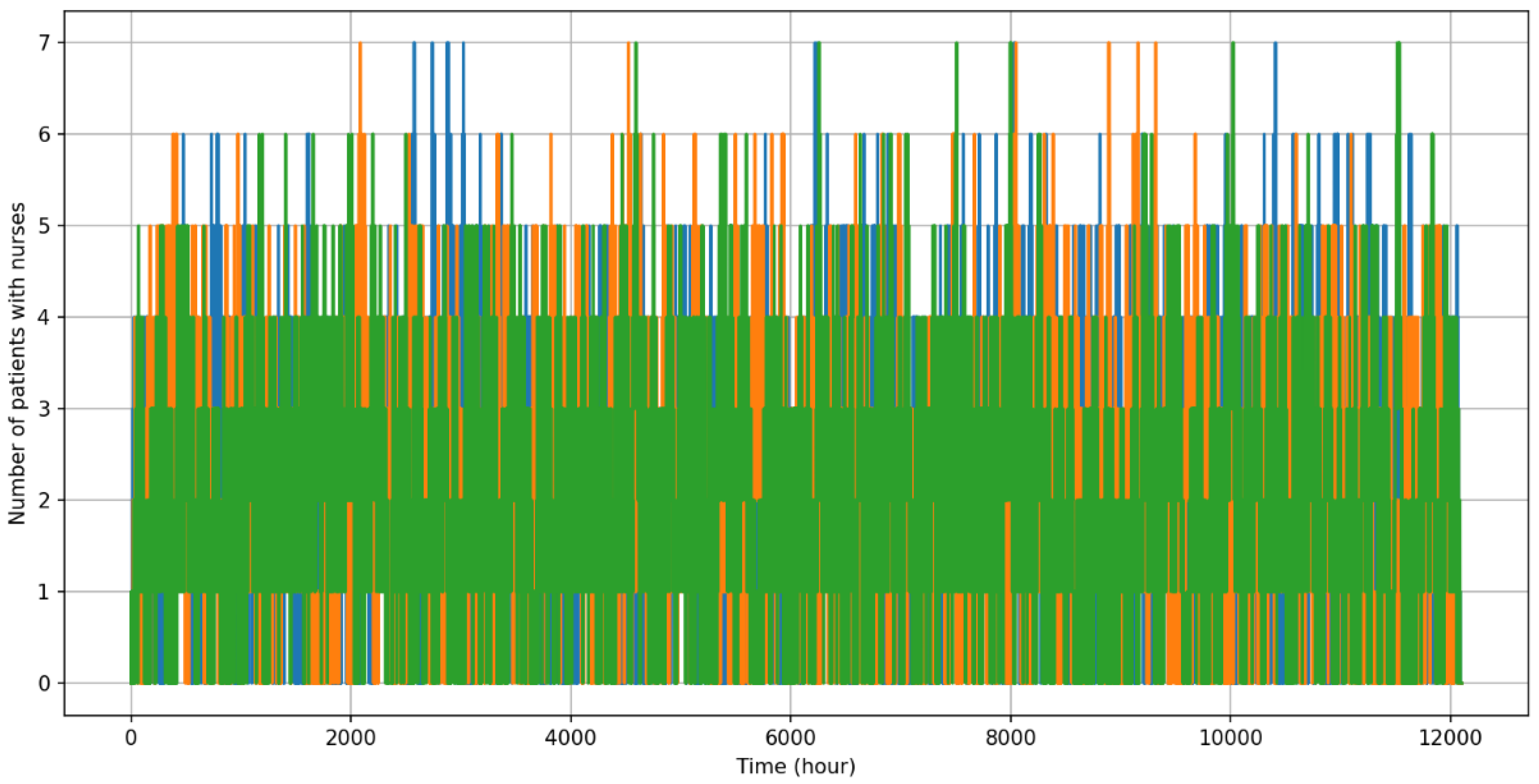
4.2.1. Scenario Generation: Coordination in Different Levels of Occupancy

The coordination system for the nurses in the obstetrics department is organized as follows: generally, six nurses are available to manage the 22 beds. To optimize coordination, the nurses divide the patients into groups, ensuring that two nurses always work in proximity. This arrangement creates three teams of patients. Coordination is primarily carried out within each team, meaning that two nurses coordinate their tasks. If the workload at any given moment exceeds the workload that two nurses can handle, one nurse seeks assistance from a nurse in another team. This coordination can trigger further coordination activities. For instance, the nurse who is approached for assistance may need to consult with their teammate, or it could be that no nurse in the approached team is available, thus requiring the involvement of another team. The workload and length of stay for a patient are unknown prior to admission, introducing an additional layer of unpredictability. Moreover, the number of patients requiring admission on any given day is also uncertain, contributing to the overall variability of the system. The clinic’s maximum capacity for admissions is limited by the available induction capacity, which restricts the number of inductions to a maximum of eight per 24 h. The number of patients admitted varies between zero and eight per day. If the clinic reaches full capacity or the maximum induction limit is reached, additional patients are referred to a different hospital.

4.2.2. Model Description

The described model focuses on measuring the need for coordination, instead of the workload. Patient admissions and lengths of stay (LoS) are represented as Poisson processes, with an average interarrival time of three hours and an average LoS of 38 h. Assigning patients to teams is arbitrary, as the expected workload is not known in advance. Therefore, it is essential that nurses from different teams assist each other. The demand for care by a nurse is determined by patients per hour, with the rate set at 0.5 to introduce a high level of randomness in care requirements. The capacity needed for coordination is measured in terms of edges, representing the communication between pairs of nurses within and across teams. Coordination is required when two or more patients within the same group require nursing attention concurrently, resulting in a demand that exceeds the available nurse capacity. In such instances, nurses from other teams coordinate to facilitate the transfer of a nurse to provide assistance, thereby ensuring that patient needs are met. Once the transferred nurse completes the task, they return to their original team. Therefore, if all groups require the same level of attention, no transfers are necessary.

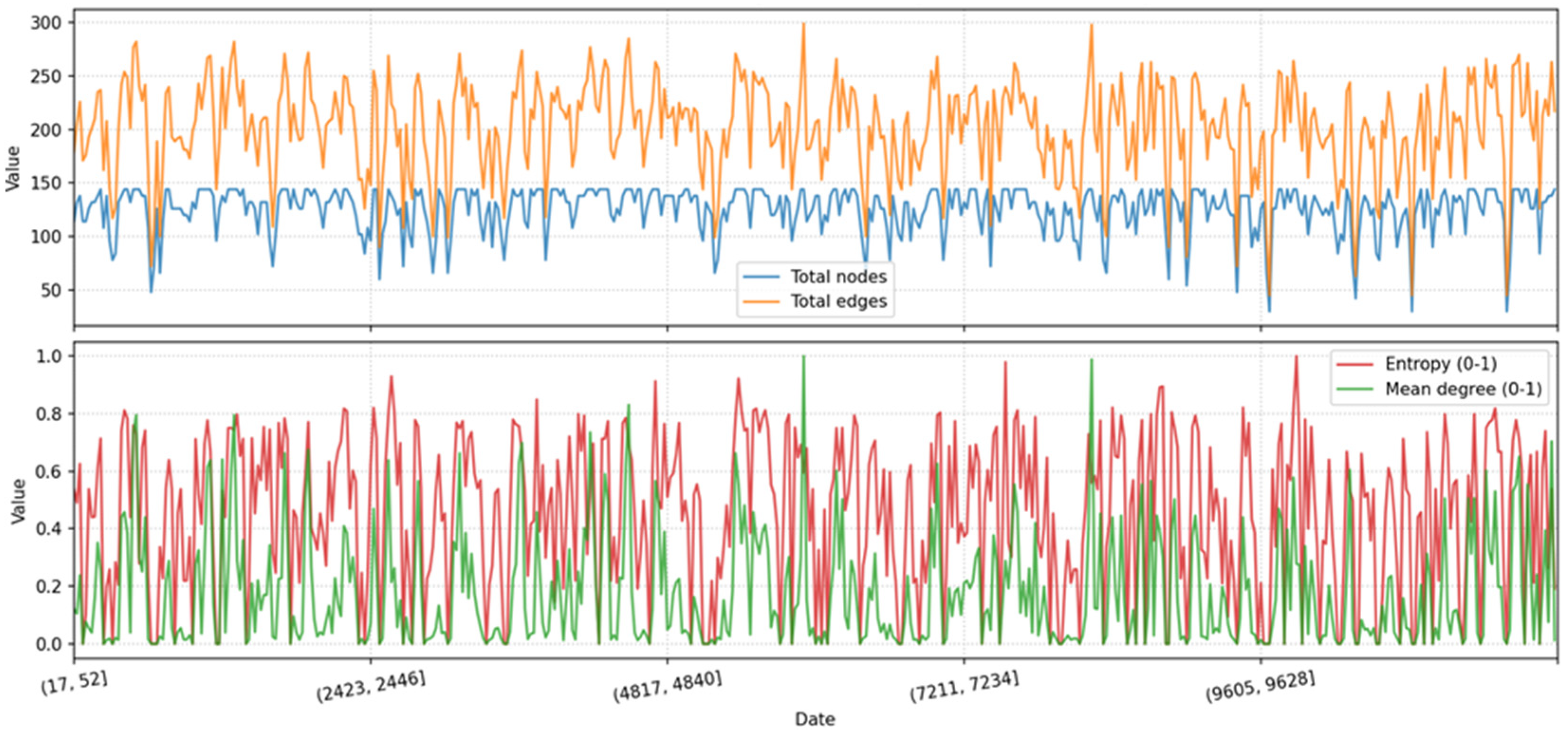
4.2.3. Simulation Results

A simulation of 500 days (12,000 h) of coordination in a three-segment obstetrics ward is presented here. The number of patients requiring nurses was calculated in hourly intervals, shown in Figure 4. As observed, the patient demand for nurses exhibits substantial variability across different segments over time, underscoring the need for coordination and highlighting the importance of system design, as previously discussed. The application of coordination rules leads to the formation of coordination networks, subsequently analyzed with the method presented in this study.
In the resulting coordination networks, patients are represented as nodes and nurse communications as edges. The system remains coordinated at all times: when a nurse needs help, they first seek assistance from available nurses within their own segment; if none are available, they reach out to another segment; if successful, the nurse responding to the request becomes unavailable to their own segment for a period of time. Thus, when additional help is required, another team is immediately approached, enabling the system to maintain coordination and respond to changing demands.
The aggregated analysis of the resulting networks considering 24 h intervals is shown in Figure 5. As expected, the number nodes and edges in the networks are positively correlated, indicating that an increase in patient numbers leads to a higher workload and a greater likelihood of nurses needing to assist each other. The entropy values in these networks range from 0.92 to 2.22, while the average degrees vary between 3.00 and 4.15. The entropy in this system is consistently above zero, while the maximum degree fluctuates between seven and nine throughout time. In only 58 times (11.6%), a maximum degree of seven was observed, while in all 442 other instances (86.4%), it reached a value of nine. Most importantly, the lowest entropy value occurs only when the maximum node degree is seven, indicating that the most predictable coordination structure is only achieved with limited connections between nurses.
Table 6 shows that the entropy of coordination remains consistently above zero, with most values falling within moderate ranges (green and orange areas). The mean degrees also tend to be generally moderate, though both entropy and average degree values exhibit significant variation. Lastly, as shown in Figure 6, the number of both nodes and edges is high when many patients are admitted, which expectedly increases the likelihood that entropy will rise. However, even with the same number of nodes and edges (indicating a similar ‘need for help’), entropy values may vary depending on how this need is distributed over time. As observed, although entropy does not exhibit high levels in this system, coordination is always required, which is often not necessary in the TPS example.

5. Discussion

Coordination of production systems can be highly complex; this study demonstrates that constraints play a significant role in reducing this complexity. Effective system design aims to balance the reduction in coordination complexity with the need for flexibility, using constraints to simplify coordination while maintaining adaptability. To evaluate this complexity, the physical and coordination networks of a production system are separated, and entropy measures are employed in combination with node influence metrics, an approach that has been proven valuable in previous research.
Two production systems with vastly different arrival patterns for orders and services were analyzed: a highly predictable Toyota Production System (TPS), characterized by a high design complexity, and an obstetrics clinic, characterized by a high uncertainty in patient arrivals and throughput times, yet a relatively low design complexity. We further model the coordination network as a series of temporal networks, enabling a deeper understanding of the timing, frequency, and forms of coordination that arise.

5.1. Differences in Entropy and Network Metrics Among TPS and the Obstetrics Clinic

In the TPS, coordination networks rarely develop, and are only activated in response to well-defined, unfavorable events. These networks can be described using metrics such as entropy, average degree, and maximum degree of nodes. The values of these metrics are limited and closely related, with the interplay between average and maximum degree indicating the level of centralization of coordination at specific nodes, i.e., units within the production system. When coordination relies mostly on adjacent nodes, as in the TPS ’need help’ scenario or among nurses in the obstetrics clinic, temporal networks can form with coordination concentrated at particular nodes, leading to centralization. This requires these central nodes to have sufficient capacity to handle the coordination. This can be problematic as it is uncertain in adjacent coordination networks which nodes will become central.
As it is uncertain in adjacent coordination networks which nodes will become central, all nodes should be equipped with the necessary capacity and skills to take on this responsibility. If this is not feasible, it is recommended to avoid adjacent coordination or shift to andon coordination shortly after ’need help’ triggers adjacent coordination. In the obstetrics clinic, where only adjacent coordination occurs, the low control over admissions and workload results in the constant activation of temporal coordination networks that are always connected. In this example, the outcome is that there is never a situation without entropy, as many nodes are always involved in the coordination process.

5.2. Design Complexity: Open Versus Closed Loop Systems

The obstetrics clinic example resembles a push system of type (a), and the TPS example, a pull system of types (f) and (g), according to the typology presented in Appendix A. In a push system work is scheduled based on demand, whereas in a pull system, it is authorized based on its current status [53]. Open-loop systems, like the obstetrics clinic, face challenges in utilizing feedback and taking action to optimize workflow [49] (p. 59), as important information necessary for maintaining control over the production system is either unavailable or not used effectively. As a result, the interdependence between demand and production is insufficiently managed in such systems, and the entropy of demand is not sufficiently reduced, requiring slack capacity to accommodate variability in production and coordination.
In network terms, not defining constraints on the development of the coordination network can lead to emergent constraints and potential capacity loss. High entropy and high maximum degree nodes in coordination networks indicate emergent constraints and suggest a lack of control over them. In such cases, the coordination network itself imposes limitations on the system’s capacity. This lack of control over coordination can lead to inefficiencies, as the system struggles to adapt to unforeseen demands or changes in the environment. In contrast, pull systems, such as TPS, manage coordination more effectively by continuously adjusting based on real-time system feedback. This approach reduces the likelihood of emergent constraints and minimizes the need for slack capacity. The ability to adapt quickly to changes in demand and production status is therefore a key advantage of pull systems over push systems, especially in environments with higher uncertainty.

5.3. Crises and Shocks

This study primarily focuses on entropy measures within stable production systems and does not account for economic shocks, sudden sourcing shortages, or other out-of-scope events. Understanding how production systems respond to crises and shocks warrants future investigation, which may likewise utilize entropy and production system metrics to evaluate more dynamic conditions.

5.4. Entropy Methods

Shannon entropy was chosen to measure the complexity of coordination in this study, although alternative entropy methods may also be employed for the same purpose. Notably, Jensen–Shannon divergence has been used in Network Portrait Divergence analysis [54,55,56], especially in the life sciences, to establish a ranking of distinct graphs, in which edges may be weighted. A similar approach could potentially extend the methodology presented in this article, for instance, to incorporate information on the physical distance between nodes in the coordination network as edge weights, enabling the consideration of additional factors in their analysis.

5.5. Limitations and Future Research

The content of the edges in the coordination network is not examined in this study. However, future research could benefit from incorporating edge content to improve on their analysis. Moreover, considering the duration of temporal coordination networks would allow accounting for switching events, such as when situational coordination transitions into andon coordination after a specific time limit is exceeded. Future research may also explore the potential for defining additional switching events based on actual coordination entropy, where the type of coordination changes in response to reaching a certain threshold.
This study also does not investigate the consequences of coordination on capacity utilization, a crucial area that warrants further research. As coordination affects overall system capacity, examining these consequences is therefore an essential task. The optimal amount of slack time likewise requires further investigation, particularly in healthcare settings such as the one presented. Beyond its importance for efficient care delivery, a lack of slack can increase stress and dissatisfaction among healthcare professionals, leading them to feel a loss of autonomy and ultimately contributing to their decision to leave their job [57].

6. Conclusions

This article introduces a novel method for modeling and analyzing coordination systems such as temporal networks, leveraging Shannon entropy and node influence metrics to uncover the complexities of coordination dynamics. The proposed approach was applied to two diverse case studies, allowing a comparative analysis of a Toyota Production System and a university obstetric clinic, yielding valuable insights into their distinct network structures and behaviors.
In the TPS example, zero-entropy situations occurred in 38.40% of ‘need help’ time windows, characterized by local coordination. In contrast, andon coordination exhibited zero entropy in 76.62% of all situations. The highest entropy values were observed in the ‘need help’ time windows. Notably, outside of zero-entropy situations, andon coordination networks had higher average and maximum node degrees compared to ‘need help’ coordination networks. This suggests that andon networks exhibit a more organized concentration of nodes that fulfill a coordination function. As the ‘need help’ time windows increase in duration, the likelihood of uncontrolled coordination networks emerging also grows. Therefore, the ’need help’ time windows should be sufficiently long to facilitate adjacent coordination yet constrained in time to minimize the odds of uncontrolled networks arising.
In the university obstetric clinic, only local coordination occurs frequently and is relatively unconstrained. Observed entropy values ranged between 0.92 and 2.23, whereas average degrees varied between 3 and 4.08 indicating that coordination needs typically involve more than two nurses. This is a notable difference from the TPS example, where coordination needs are generally low for most of the time, while in the obstetric clinic, coordination needs are consistently higher.
The comparative analysis of the two case studies reveals distinct characteristics of coordination systems, highlighting the importance of context and system-specific factors in shaping network dynamics and ultimately enabling a well-informed system design. Future research can build on these findings to explore the implications of these dynamics in various domains, and to develop more nuanced understandings of the complex relationships that underlie effective coordination.

Author Contributions

F.v.M.: conceptualization, methodology, software, model development, manuscript writing, and reviewer comment-based revisions. H.B.: conceptualization, manuscript reviewing. F.T.: validation, manuscript reviewing. N.A.R.d.A.P.: software, model development, manuscript reviewing. W.W.: manuscript reviewing. A.v.d.H.: conceptualization, manuscript writing, and reviewer comment-based revisions. All authors have read and agreed to the published version of the manuscript.

Funding

This research received no funding.

Institutional Review Board Statement

Not applicable.

Informed Consent Statement

Not applicable.

Data Availability Statement

This is a theoretical study. All data are simulated with the models described in the manuscript.

Conflicts of Interest

The authors declare no conflicts of interest.

Appendix A

Typology of coordination networks for production systems. The systems described from (a) to (g) represent production systems that utilize feedforward and feedback loops to measure the status of workstations and work in progress. Note that this typology refers only to production line systems, not job shop (“criss-cross”) systems, although systems (e) and (g) may also be applied to job shop systems.
Physical and Information FlowsType of Coordination Network
Logistics 09 00046 i001(a) No feedback loops. Products and materials flow from upstream stations to downstream stations once ready, independent of the status of the downstream stations. No information is sent upstream, and no coordination occurs.
Logistics 09 00046 i002(b) Local feedback loops. Downstream stations communicate their status to the next upstream workstations, enabling adjustments to their operations. Coordination occurs via local feedback loops, and if feedback times are short, this coordination can operate nearly in real-time at the system level.
Logistics 09 00046 i003
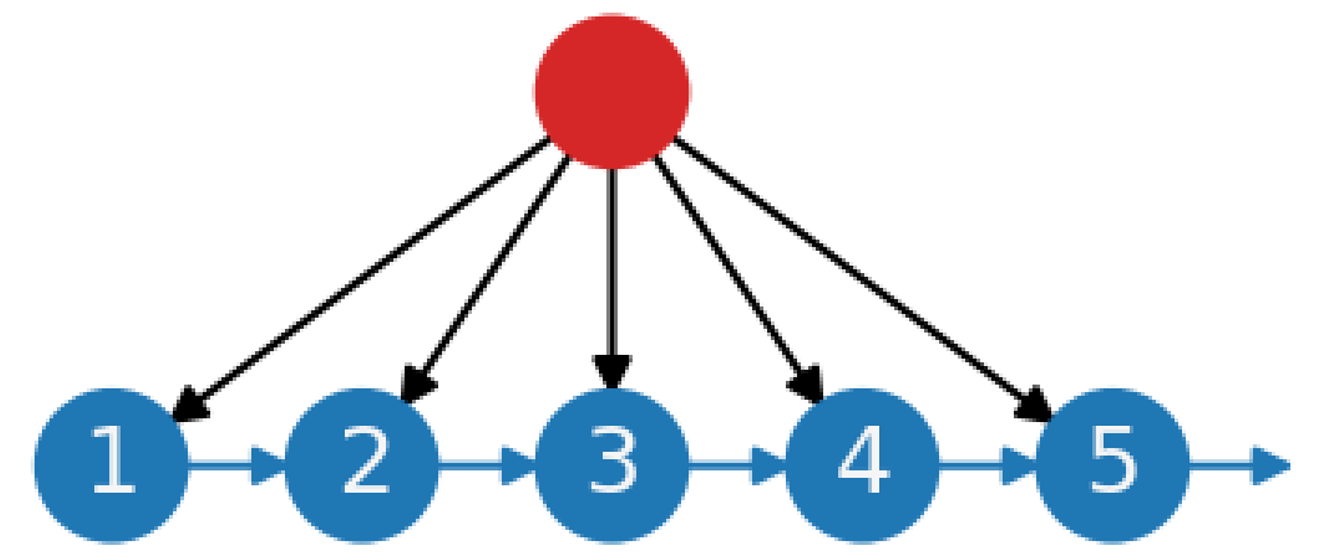
(c) Central planning without feedback loops. Similar to (a), but with an added central planning function. The planning function has two roles: (1) production leveling: determining the volume, mix, and order of products to meet demand and smooth the workload; and (2) capacity assignment: allocating capacity to workstations. Communication between upstream and downstream stations is absent, and coordination is achieved centrally. This system works best when operations are deterministic. If operations are not fully deterministic, slack capacity must be available at each workstation, and waiting times between workstations should be allowed. Slack capacity and waiting times serve as buffers, but their extent is difficult to predict.
Logistics 09 00046 i004
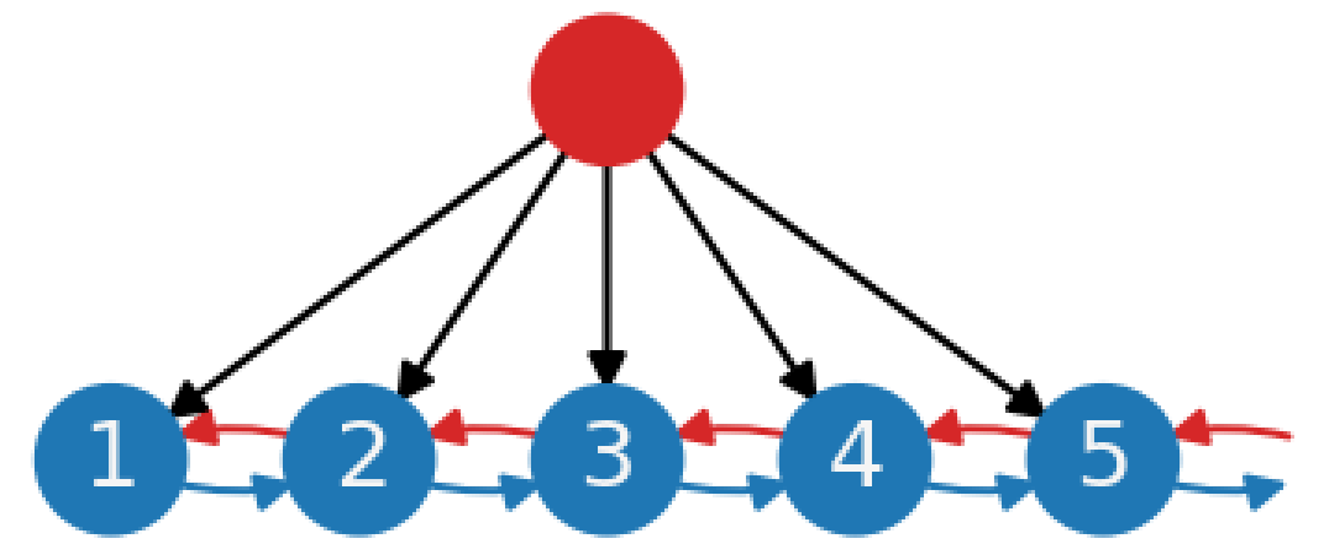
(d) Central planning with local feedback loops. Combination of (b) and (c). The planning function is the same as in (c), but operational coordination is achieved entirely through local feedback loops. This system is especially useful for production systems with many product variants. Unlike (c), slack capacity and waiting times between workstations are controlled locally.
Logistics 09 00046 i005
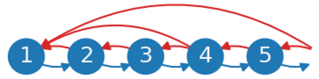
(e) Local and global feedback loops. This system builds on (b) by incorporating work-in-progress coordination. Order release is influenced by the total amount of work in progress from the last station to the first (upper red line). It is also possible to measure and communicate the workload between the first workstation and an intermediate station to the beginning of the chain (middle red line). This addition of global control to the local feedback loops, contrasting with (b), allows upstream stations to adjust their workload based on downstream constraints, implying the need for assistance from workers from adjacent stations. The extent to which this is possible depends on whether the standard workload plus a surplus factor (including slack) is below a predefined threshold. If this threshold is exceeded, the release of orders stops.
Logistics 09 00046 i006(f) Central planning with local and global feedback loops. Combination of (c) and (e), used for work-in-progress coordination. As in (d), the rationale for the planning loop (in black) is to be found in occasions when many different product variants are to be produced, allowing for the central relocation of workers.
Logistics 09 00046 i007
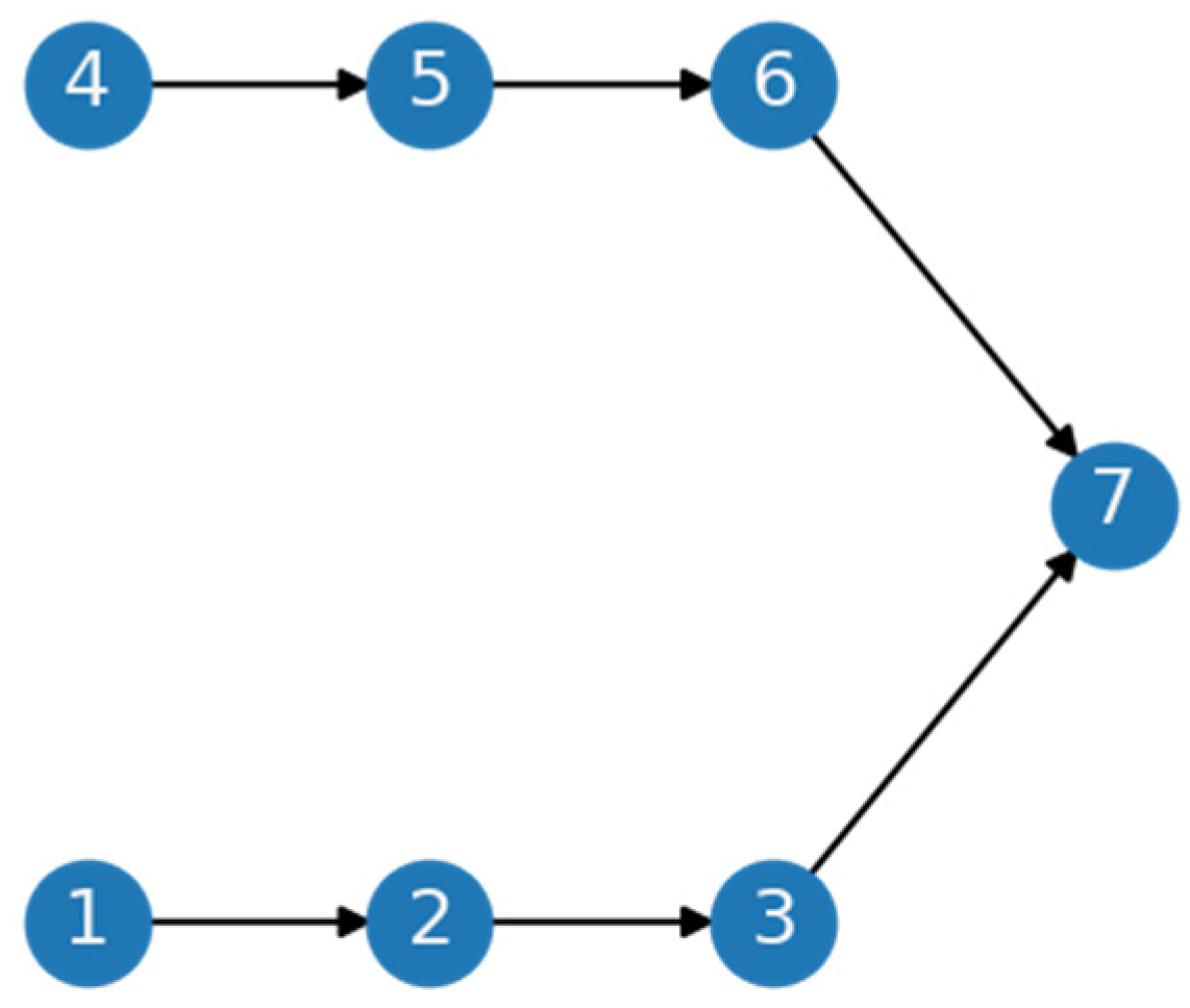
(g) Local and global feedback loops with synchronization. Similar to (e), but applied to multiple production lines. Work in progress is measured from workstations 1 to 4, from workstations ’a’ to 4, from the first to the defined ‘end station’, and from ‘a’ to the ‘end station’. In total, four work-in-progress measurements are used to control the production system. With multiple production lines, synchronization between these lines is necessary. This means that the release of orders across different production lines must be coordinated (e.g., at workstations 1 and ’a’). This system also allows workers from adjacent workstations on different production lines to assist each other.

References

  1. Zhu, X.; Hu, S.J.; Koren, Y.; Marin, S.P. Modeling of Manufacturing Complexity in Mixed-Model Assembly Lines. J. Manuf. Sci. Eng. 2008, 130, 051013. [Google Scholar] [CrossRef]
  2. Hu, S.J.; Zhu, X.; Wang, H.; Koren, Y. Product variety and manufacturing complexity in assembly systems and supply chains. CIRP Ann. —Manuf. Technol. 2008, 57, 45–48. [Google Scholar] [CrossRef]
  3. Chryssolouris, G.; Efthymiou, K.; Papakostas, N.; Mourtzis, D.; Pagoropoulos, A. Flexibility and complexity: Is it a trade-off? Int. J. Prod. Res. 2013, 51, 6788–6802. [Google Scholar] [CrossRef]
  4. Ivanov, D. Two views of supply chain resilience. Int. J. Prod. Res. 2024, 62, 4031–4045. [Google Scholar] [CrossRef]
  5. Aldrighetti, R.; Calzavara, M.; Martignago, M.; Zennaro, I.; Battini, D.; Ivanov, D.A. methodological framework for the design of efficient resilience in supply networks. Int. J. Prod. Res. 2024, 62, 271–290. [Google Scholar] [CrossRef]
  6. Aldrighetti, R.; Battini, D.; Ivanov, D. Efficient resilience portfolio design in the supply chain with consideration of preparedness and recovery investments. Omega 2023, 117, 102841. [Google Scholar] [CrossRef]
  7. Riccardo, A.; Daria, B.; Dmitry, I. Increasing supply chain resilience through efficient redundancy allocation: A risk-averse mathematical model. IFAC-Pap. 2021, 54, 1011–1016. [Google Scholar] [CrossRef]
  8. Aldrighetti, R.; Battini, D.; Ivanov, D.; Zennaro, I. Costs of resilience and disruptions in supply chain network design models: A review and future research directions. Int. J. Prod. Econ. 2021, 235, 108103. [Google Scholar] [CrossRef]
  9. Bonchev, D.; Rouvray, D. Shannon’s information and complexity. Complex. Chem. Introd. Fundam. 2003, 7, 157–187. [Google Scholar]
  10. Dehmer, M.; Mowshowitz, A. A history of graph entropy measures. Inf. Sci. 2011, 181, 57–78. [Google Scholar] [CrossRef]
  11. Benjamin, A.; Chartrand, G.; Zhang, P. The Fascinating World of Graph Theory; University Press: Princeton, NJ, USA, 2015. [Google Scholar]
  12. Kumar, V. Entropic measures of manufacturing flexibility. Int. J. Prod. Res. 1987, 25, 957–966. [Google Scholar] [CrossRef]
  13. Battini, D.; Persona, A.; Allesina, S. Towards a use of network analysis: Quantifying the complexity of Supply Chain Networks. Int. J. Electron. Cust. Relatsh. Manag. 2007, 1, 75–90. [Google Scholar] [CrossRef]
  14. Wang, J.; Wilson, R.C.; Hancock, E.R. Network edge entropy decomposition with spin statistics. Pattern Recognit. 2021, 118, 108040. [Google Scholar] [CrossRef]
  15. Cheng, C.-Y.; Chen, T.-L.; Chen, Y.-Y. An analysis of the structural complexity of supply chain networks. Appl. Math. Model. 2014, 38, 2328–2344. [Google Scholar] [CrossRef]
  16. Morzy, M.; Kajdanowicz, T.; Kazienko, P. On measuring the complexity of networks: Kolmogorov complexity versus entropy. Complexity 2017, 2017, 3250301. [Google Scholar] [CrossRef]
  17. Chaitin, G.J. Algorithmic Information Theory. IBM J. Res. Dev. 1977, 21, 350–359. [Google Scholar] [CrossRef]
  18. Gell-Mann, M. The Quark and the Jaguar: Adventures in the Simple and the Complex; St. Martin’s Press: New York, NY, USA, 1995. [Google Scholar]
  19. Gell-Mann, M.; Lloyd, S. Information measures, effective complexity, and total information. Complexity 1996, 2, 44–52. [Google Scholar] [CrossRef]
  20. Zenil, H.; Kiani, N.A.; Tegnér, J. A Review of Graph and Network Complexity from an Algorithmic Information Perspective. Entropy 2018, 20, 551. [Google Scholar] [CrossRef]
  21. Martignago, M.; Calzavara, M.; Katiraee, N.; Battini, D. Entropic measurement in supply chain network: Past applications, current trends, and future research. In Proceedings of the Summer School Francesco Turco, Genova, Italy, 6–8 September 2023; Volume 1, pp. 1–7. [Google Scholar]
  22. Carcassi, G.; Aidala, C.A.; Barbour, J. Variability as a better characterization of Shannon entropy. Eur. J. Phys. 2021, 42, 045102. [Google Scholar] [CrossRef]
  23. Lin, Y.H.; Wang, Y.; Lee, L.H.; Chew, E.P. Consistency matters: Revisiting the structural complexity for supply chain networks. Phys. A Stat. Mech. Its Appl. 2021, 572, 125862. [Google Scholar] [CrossRef]
  24. Shannon, C.E. A mathematical theory of communication. Bell Syst. Tech. J. 1948, 27, 379–423. [Google Scholar] [CrossRef]
  25. Monostori, J. Robustness- and Complexity-oriented Characterization of Supply Networks’ Structures. Procedia CIRP 2016, 57, 67–72. [Google Scholar] [CrossRef]
  26. Womack, J.P.; Jones, D.T. Lean Thinking—Banish Waste and Create Wealth in Your Corporation; Revised and Updated; Free Press: New York, NY, USA, 2003. [Google Scholar]
  27. Nye, D.E. America’s Assembly Line; The MIT Press: Cambridge, MA, USA, 2013. [Google Scholar]
  28. Katiraee, N.; Calzavara, M.; Finco, S.; Battaïa, O.; Battini, D. Assembly line balancing and worker assignment considering workers’ expertise and perceived physical effort. Int. J. Prod. Res. 2023, 61, 6939–6959. [Google Scholar] [CrossRef]
  29. Liu, C.; González, V.A.; Pavez, I.; Tortorella, G.L.; Abdelmegid, M. Exploring the socio-technical interactions associated with lean implementation: A systematic literature review. Prod. Plan. Control. 2025, 1–33. [Google Scholar] [CrossRef]
  30. Khakifirooz, M.; Fathi, M.; Dolgui, A.; Pardalos, P.M. Assessing resiliency in scale-free supply chain networks: A stress testing approach based on entropy measurements and value-at-risk analysis. Int. J. Prod. Res. 2024, 1–34. [Google Scholar] [CrossRef]
  31. Sharma, S.K.; Srivastava, P.R.; Kumar, A.; Jindal, A.; Gupta, S. Supply chain vulnerability assessment for manufacturing industry. Ann. Oper. Res. 2023, 326, 653–683. [Google Scholar] [CrossRef]
  32. Van Rossum, G.; Drake, F.L., Jr. The Python Language Reference; Python Software Foundation: Wilmington, DE, USA, 2014. [Google Scholar]
  33. The Pandas Development Team. pandas-dev/pandas: Pandas 2.2.3; Zenodo: Genève, Switzerland, 2021. [Google Scholar]
  34. McKinney, W. Data Structures for Statistical Computing in Python. In Proceedings of the 9th Python in Science Conference, Austin, TX, USA, 28 June–3 July 2010; Walt, S.É.V.D., Millma, J., Eds.; scipy.org: Austin, TX, USA, 2010; pp. 56–61. [Google Scholar]
  35. Caswell, T.A.; Droettboom, M.; Lee, A.; Sales De Andrade, E.; Hoffmann, T.; Hunter, J.; Klymak, J.; Firing, E.; Stansby, D.; Varoquaux, N.; et al. matplotlib/matplotlib: REL, v3.5.2; Zenodo: Genève, Switzerland, 2022. [Google Scholar]
  36. Hunter, J.D. Matplotlib: A 2D Graphics Environment. Comput. Sci. Eng. 2007, 9, 90–95. [Google Scholar] [CrossRef]
  37. Plotly_Technologies. Plotly Open Source Graphing Library for Python. 2023. Available online: https://plotly.com/python/?_ga=2.202387800.891488512.1698351200-1657284833.1677516886 (accessed on 27 October 2023).
  38. Sievert, C. Interactive Web-Based Data Visualization with R, Plotly, and Shiny; CRC Press: Boca Raton, FL, USA, 2020. [Google Scholar]
  39. Harris, C.R.; Millman, K.J.; Van Der Walt, S.J.; Gommers, R.; Virtanen, P.; Cournapeau, D.; Wieser, E.; Taylor, J.; Berg, S.; Smith, N.J.; et al. Array programming with NumPy. Nature 2020, 585, 357–362. [Google Scholar] [CrossRef]
  40. Hagberg, A.; Schult, D.; Swart, P. Networkx, Version 2.8; NetworkX Developers: Los Alamos, NM, USA, 2022.
  41. Hagberg, A.; Swart, P.; Chult, D.S. Exploring Network Structure, Dynamics, and Function Using NetworkX; Los Alamos National Lab. (LANL): Los Alamos, NM, USA, 2008. [Google Scholar]
  42. Passos, N.A.R.A.; Carlini, E.; Trani, S. NetworkX-Temporal: Building, Manipulating, and Analyzing Dynamic Graph Structures; Zenodo: Genève, Switzerland, 2024. [Google Scholar]
  43. Liker, J.K.; Meier, D. The Toyota Way Field Book; Tata McGraw-Hill Publishing Company: New Delhi, India, 2006; p. 475. [Google Scholar]
  44. Black, J.T. Design rules for implementing the Toyota Production System. Int. J. Prod. Res. 2007, 45, 3639–3664. [Google Scholar] [CrossRef]
  45. Mönch, T.; Huchzermeier, A.; Bebersdorf, P. Variable takt times in mixed-model assembly line balancing with random customisation. Int. J. Prod. Res. 2021, 59, 4670–4689. [Google Scholar] [CrossRef]
  46. Mönch, T.; Huchzermeier, A.; Bebersdorf, P. Variable takt time groups and workload equilibrium. Int. J. Prod. Res. 2020, 60, 1535–1552. [Google Scholar] [CrossRef]
  47. Munavalli, J.R.; Vasudevarao, S.; Srinivasan, A.; Manjunath, U.; van Merode, G.G. A Robust Predictive Resource Planning under Demand Uncertainty to Improve Waiting Times in Outpatient Clinics. J. Health Manag. 2017, 19, 563–583. [Google Scholar] [CrossRef] [PubMed]
  48. Munavalli, J.R.; Rao, S.V.; Srinivasan, A.; van Merode, G.G. intelligent real-time scheduler for out-patient clinics: A multi-agent system model. Health Inform. J. 2020, 26, 2383–2406. [Google Scholar] [CrossRef] [PubMed]
  49. Munavalli, J.R.; Boersma, H.J.; Rao, S.V.; van Merode, G.G. Real-Time Capacity Management and Patient Flow Optimization in Hospitals Using AI Methods. In Artificial Intelligence and Data Mining in Healthcare; Masmoudi, M., Jarboui, B., Siarry, P., Eds.; Springer International Publishing: Cham, Switzerland, 2021; pp. 55–69. [Google Scholar]
  50. Masuda, N.; Holme, P. Detecting sequences of system states in temporal networks. Sci. Rep. 2019, 9, 795. [Google Scholar] [CrossRef] [PubMed]
  51. Moctar, A.O.M.; Sarr, I.; Tanzouak, J.V. Snapshot Setting for Temporal Networks Analysis. In e-Infrastructure and e-Services for Developing Countries; Springer International Publishing: Cham, Switzerland, 2019. [Google Scholar]
  52. Bushuyev, S.D.; Sochnev, S.V. Entropy measurement as a project control tool. Int. J. Proj. Manag. 1999, 17, 343–350. [Google Scholar] [CrossRef]
  53. Hopp, W.J.; Spearman, M.L. Factory Physics: Foundations of Manufacturing Management, 2nd ed.; Irwin/McGraw-Hill: New York, NY, USA, 2001. [Google Scholar]
  54. Meng, K.; Ba, Z.; Liu, L. A Network Portrait Divergence Approach to Measure Science-Technology Linkages; Springer Nature: Cham, Switzerland, 2024. [Google Scholar]
  55. Bagrow, J.P.; Bollt, E.M. An information-theoretic, all-scales approach to comparing networks. Appl. Netw. Sci. 2019, 4, 45. [Google Scholar] [CrossRef]
  56. Bagrow, J.P.; Bollt, E.M.; Skufca, J.D.; ben-Avraham, D. Portraits of complex networks. Europhys. Lett. 2008, 81, 68004. [Google Scholar] [CrossRef]
  57. Van Merode, F.; Groot, W.; Somers, M. Slack Is Needed to Solve the Shortage of Nurses. Healthcare 2024, 12, 220. [Google Scholar] [CrossRef]
Figure 1. Example of a TPS network at factory level.
Logistics 09 00046 g001
Figure 2. (a,b). Snapshots of example Takttime periods displaying all 7 workstations. Top (a): coordination between workstation 2 and adjacent workstations 1 and 3 is requested at help time. Bottom (b): all workstations stop to help workstation 6 as it reaches andon time.
Logistics 09 00046 g002
Figure 3. (ac). Networks of workstations providing and receiving assistance. Graph representations of static (a) and temporal (b,c) networks at different coordination times.
Logistics 09 00046 g003
Figure 4. Simulation of patients staying at the three segments of the clinic and their need for nurses, considering hourly periods. Each segment is represented by a distinct color (blue, orange, and green). The number of patients shown are per segment (the bars are unstacked).
Logistics 09 00046 g004
Figure 5. Simulation of 500 days of coordination of the obstetrics ward, considering 24 h periods. Top: number of patients (nodes) and edges (nurse communications). Bottom: normalized entropy and mean degree values, ranging from 3.00 (0.0) to 4.15 (1.0).
Logistics 09 00046 g005
Figure 6. Entropy in relation to other variables of interest. Left: relationship between the total number of nodes, edges, and entropy. Colors represent the mean degree for each situation (24 h). Right: relationship between the total number of patients at each hour, summed over 24 h, the number of nodes, and entropy, with the average degree shown in the left image.
Logistics 09 00046 g006
Table 1. Topics addressed per section.
SectionTopics Addressed
2. Coordination and network entropyHow can coordination be modeled as networks?
To what extent can entropy of these networks measure the coordination complexity?
3. Graph theory to describe network and situation entropyWhat types of coordination complexity do occur?
Where do these occur in coordination networks?
How can coordination networks be simulated?
What are the metrics used to evaluate the characteristics of coordination networks?
4. Two examples of coordination systemsIntroduction of concepts of Takttime, adjacent and andon coordination and temporal coordination networks
Comparison of coordination of Toyota Production System (TPS) with University Obstetric Clinic
Simulation of scenarios for both examples
5. DiscussionWhat are the differences between the coordination networks of TPS and the University Obstetric Clinic?
What do these differences mean?
What is the design complexity of the TPS and the University Obstetric Clinic?
Limitation of this study
6. ConclusionsWhat is the insight into the complexity of coordination in both examples?
Table 2. Variables describing coordination networks of production systems.
VariableMeaning
Number of nodesThe number of agents (such as workers, machines, or entities) involved in coordination within the system.
Number of edgesThe total number of coordination links (connections) between the nodes in the network.
Node degreeThe sum of incoming and outgoing edges associated with a node. It signals the relative involvement of a node in the coordination network.
Average node degreeThe mean degree of all nodes in the network, i.e., the total number of edges divided by the total number of nodes in the graph.
Maximum node degreeThe highest degree among all the nodes in the network, indicating the most involved agent in coordination. The difference between the average and maximum degree of nodes is used to measure the centralization of coordination within the network.
EntropyIn this context, entropy refers to graph entropy as a measure of the structural complexity of the coordination network.
Table 3. Parameters for scenarios. Note that c1 < c3, (c1 + c2) <= c3, and c3 < c4 < 5.
Parameter DescriptionParameter Value
c1Time without features (standard time)60
c2Mean extra time (due to product features or quality issues, based on uniform distribution)range (5, 25, 5)
c3Help time (trigger time for coordination from adjacent workstations, added to c2)range (5, 15, 5)
c4Andon time (trigger time for coordination from all workstations, added to c2)range (10, 25, 5)
c5Takttime (maximum time per cycle)100
Table 4. Node characteristics of possible situation coordination networks, based on all scenarios (24,000 replications).
Situation Networks (Local Coordination)
Max DegreeAverage DegreeEntropy
0.000.860.991.151.381.451.561.661.841.95
21.710.00%2.43%0.00%0.00%0.00%0.00%0.00%0.00%0.00%0.00%
2.0038.49%0.00%0.00%0.00%0.00%0.00%0.00%0.00%0.00%0.00%
32.000.00%0.00%0.00%7.09%0.00%0.00%4.64%0.00%0.00%0.00%
2.290.00%7.15%0.00%0.00%0.28%7.41%0.00%0.00%0.00%0.00%
2.570.00%0.00%1.88%0.00%0.00%0.00%0.00%0.00%0.00%0.00%
42.000.00%0.00%0.00%0.00%5.69%0.00%0.00%0.00%0.00%0.00%
2.290.00%0.00%0.00%0.00%0.00%0.00%3.34%9.31%0.00%3.04%
2.570.00%0.00%0.00%0.00%3.96%0.00%0.36%0.00%4.60%0.00%
2.860.00%0.00%0.00%0.00%0.00%0.00%0.35%0.00%0.00%0.00%
Table 5. Node characteristics of possible andon coordination networks, based on all scenarios (24,000 replications).
Andon Networks (Global Coordination)
Maximum DegreeAverage DegreeAndon Entropy
0.000.590.860.99
22.0076.62%0.00%0.00%0.00%
83.710.00%5.12%0.00%0.00%
5.140.00%0.00%6.38%0.00%
6.290.00%0.00%0.00%5.96%
7.140.00%0.00%0.00%3.68%
7.710.00%0.00%1.71%0.00%
8.000.55%0.00%0.00%0.00%
Table 6. Relation between entropy and average node degree at the obstetric clinic. The mean degree varies between 3 and 4.08. The entropy values range from 0.92 to 2.23, with 242 distinct values. The lowest entropy value occurs only when the maximum degree is 7. Entropy and average degree values have been binned into value ranges of 0.1.
Average DegreeEntropy (Normalized Between 0 and 1)
0.0–0.10.1–0.20.2–0.3]0.3–0.40.4–0.50.5–0.60.6–0.70.7–0.80.8–0.90.9–1.0
0.0–0.111.80%1.80%12.00%9.40%8.20%3.20%1.40%0.00%0.00%0.00%
0.1–0.20.00%0.60%0.00%1.40%3.20%3.20%3.20%1.80%0.20%0.00%
0.2–0.30.00%0.00%0.00%0.80%0.60%1.60%3.60%4.00%0.20%0.00%
0.3–0.40.00%0.00%0.00%0.00%0.40%0.80%1.40%3.20%0.80%0.40%
0.4–0.50.00%0.00%0.00%0.00%0.20%0.20%2.00%2.80%2.60%0.40%
0.5–0.60.00%0.00%0.00%0.00%0.00%0.00%0.20%3.40%1.40%0.20%
0.6–0.70.00%0.00%0.00%0.00%0.00%0.00%0.60%1.80%0.40%0.00%
0.7–0.80.00%0.00%0.00%0.00%0.00%0.20%0.60%2.00%0.20%0.00%
0.8–0.90.00%0.00%0.00%0.00%0.00%0.00%0.20%0.60%0.00%0.00%
0.9–1.00.00%0.00%0.00%0.00%0.00%0.20%0.60%0.00%0.00%0.00%
Disclaimer/Publisher’s Note: The statements, opinions and data contained in all publications are solely those of the individual author(s) and contributor(s) and not of MDPI and/or the editor(s). MDPI and/or the editor(s) disclaim responsibility for any injury to people or property resulting from any ideas, methods, instructions or products referred to in the content.

