
A Multi-Type Ship Allocation and Routing Model for Multi-Product Oil Distribution in Indonesia with Inventory and Cost Minimization Considerations: A Mixed-Integer Linear Programming Approach


Abstract
1. Introduction
1.1. Background
1.2. State of the Art for Solving Routing Optimization Problems
1.3. Research Gap
1.4. Objective
1.5. Contribution
2. Methods
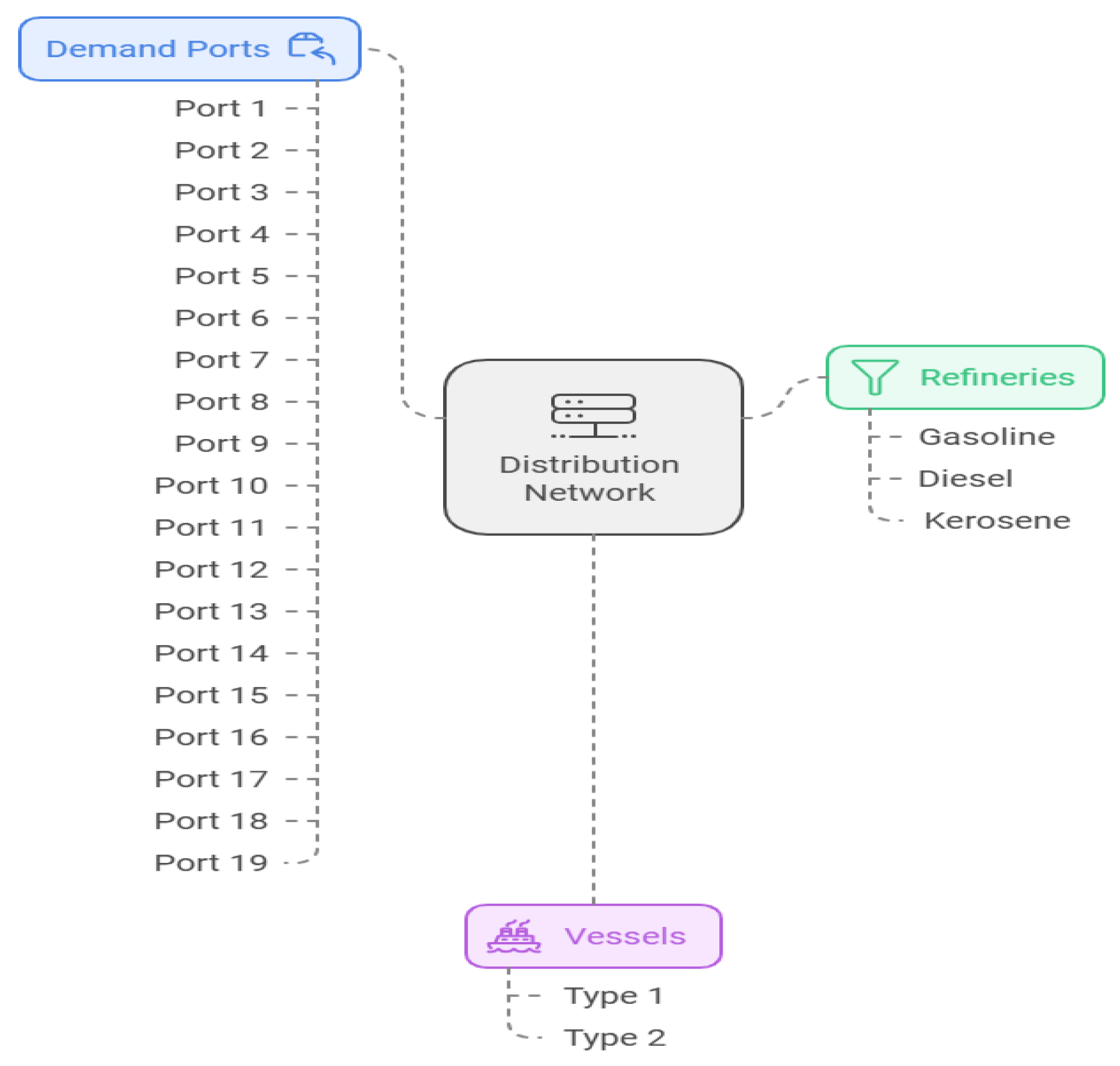
2.1. Problem Description
2.2. Mathematical Model
2.2.1. Set and Indices
Primary Set
- I = Set of supply ports (i I).
- J = Set of demand ports .
- K: Set of products (kK = {Gasoline, Diesel, Kerosene]).
- V: Set of vessel types (v ∈ V = {MR, GP}).
- T: Set of periods (t ∈ T).
- CIc: Set of supply ports in each port cluster c.
- CJc: Set of demand ports in each port cluster c.
- C: Set of all port clusters (c C = {Western, Central, Eastern}).
- M: A large constant (big-M).
2.2.2. Parameter
Supply and Demand
- : The supply capacity of product k at port i;
- : Demand for product k at port j;
- : The compartment capacity of vessel v for product k.
Time and Distance
- : Travel time from the port i to j
- : Dynamic Travel time from the port i to j
- : Port operation time at port i
- : Vessel availability factor for vessel type v.
Cost Parameters
- : Fixed transportation cost for vessel v traveling from port i to port j, carrying product k
- : Variable transportation cost per unit for vessel v transporting product k.
- : Port visit base cost for vessel type v
- : Port operation cost for port i when handling product k.
- : Base Penalty rate
- Hv: Fixed cost for using vessel type v
- : Service continuity cost for demand port j and product k.
Utilization Parameter
- μ: predefined minimum utilization factor, ensuring that vessels transport at least a certain fraction of their capacity.
- η: The upper limit on capacity utilization, ensuring that vessel operations remain within efficient levels
Weather and Seasonal Factors:
- α(t): Time-dependent congestion factor based on historical port traffic data
- β(s): Seasonal adjustment factor accounting for weather patterns
- γ(w): Weather-related delay factor updated using real-time meteorological data
2.2.3. Decision Variables
Binary Variables
- : 1 if vessel v travels from i to j carrying k in period t
- : 1 if vessel v travel from j to i carrying k in period t
- : 1 if vessel v visits port i in period t
- : 1 if vessel of type v is assigned to travel from port i to j
Continues Variables:
- : Quantity of product k delivered by vessel v from port i in period t
- : The quantity of product k delivered by vessel v to port j in period t.
- : Unmet demand of product k at port j in period t.
- : Inventory level of product k at port j in period t.
- : Number of vessels of type v required.
- : Number of vessels of cluster c required.
2.2.4. Object Function
- Transportation Cost (TC)
- 2.
- Port Operation Cost (POC)
- 3.
- Penalty Cost (PNC)
2.2.5. Constraints
- Flow Conservation
- 2.
- Supply Capacity
- 3.
- Total demand Satisfaction
- 4.
- Vessel Capacity
- 5.
- Vessel assignment
- 6.
- Vessel Usage
- 7.
- Inventory Balance
- 8.
- Vessel Utilization
- 9.
- Vessel Load Balance:
- 10.
- Cluster Constraints
- 11.
- Guarantee that the vessels are not overly assigned to each cluster
- 12.
- Port Visit
- 13.
- Route Feasibility
- 14.
- Multiple Compartment Compatibility
- 15.
- Dynamic Travel Time Integration:
- 16.
- Guarantee that a route happens only when a vehicle is used:
- 17.
- Non-negativity and Binary Constraints:
2.3. Solution Approach
- Gurobi solver for MILP optimization:
- 2.
- Model implement model:
- 3.
- Statistical experimental design for validation:
- 4.
- Statistical analysis for results verification:
2.4. Validation Framework
Framework of RSM
- 1.
- Defining the Factors and Responses
- Response: The primary response variable is cost minimization, which reflects the overall efficiency of the oil distribution system, service level optimization, and operational efficiency [27].
- 2.
- Experimental Design
- Central composite design (CCD): This design can be used to systematically explore the effects of the factors on the response. CCD allows for the estimation of a second-order polynomial model, which captures both linear and interaction effects among the factors [28]. By fitting a quadratic polynomial model to the experimental data, researchers can identify optimal conditions for minimizing costs;
- Box–Behnken design (BBD): Alternatively, BBD can be employed to optimize the same factors with fewer experimental runs. This design is particularly useful when the number of factors is limited, allowing for an efficient exploration of the design space while ensuring reliable estimates of the response surface [29].
- 3.
- Model Fitting
- : The predicted response variable (e.g., cost, yield, efficiency);
- : The intercepts term (constant baseline effect when all inputs are zero);
- : Linear coefficients representing the effect of each factor on Y;
- : The quadratic terms, modeling non-linear effects;
- : Interaction coefficients showing the combined effect of factors ;
- : Total number of input factors
- : The i-th input factor
- 4.
- Validation of the Model
- ANOVA: An analysis of variance (ANOVA) can be conducted to assess the significance of the fitted model and the individual factors. This step is crucial for determining whether the model adequately represents the data and whether the factors significantly influence the response.
- Residual analysis: Checking the residuals for normality and constant variance helps validate the assumptions of the regression model. If the model is deemed adequate, contour plots can be generated to visualize the response surface and identify the optimal conditions.
- 5.
- Identifying Optimal Conditions
- 6.
- Comparison with MILP Results
3. Case Study
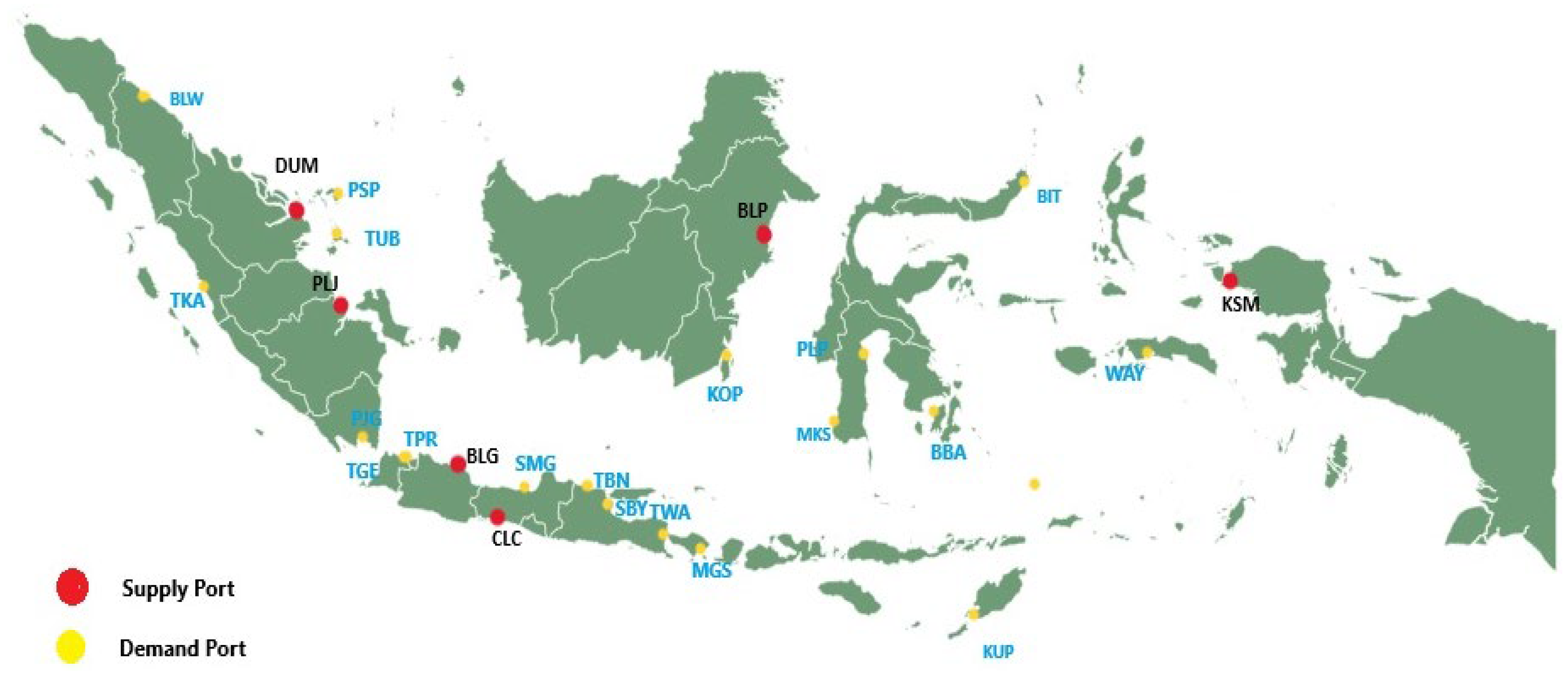
3.1. Data Collection
- Supply Port
- 2.
- Demand Port Inventory
- 3.
- Vessel and Capacity
- 4.
- Operational Cost
- 5.
- Travel Time Between Port
3.2. Application of RSM to Verify MILP Outcomes
- Defining the Factors and Responses:
- 2.
- Experimental Design
- central composite design (CCD):
- factorial point 23 = 8;
- center point = 6;
- star points 2 × 3 = 6.
- 3.
- Statistical Analysis
- ANOVA;
- regression analysis;
- respond surface generation;
- optimization method.
- 4.
- Model Validation
- R2 analysis;
- residual plot;
- normal probability plots;
- interaction effects.
4. Results
4.1. MILP Result and Outcome
4.2. Validation with Respond Surface Methodology
4.2.1. RSM Analysis, Including Response Surfaces and Contour Plots
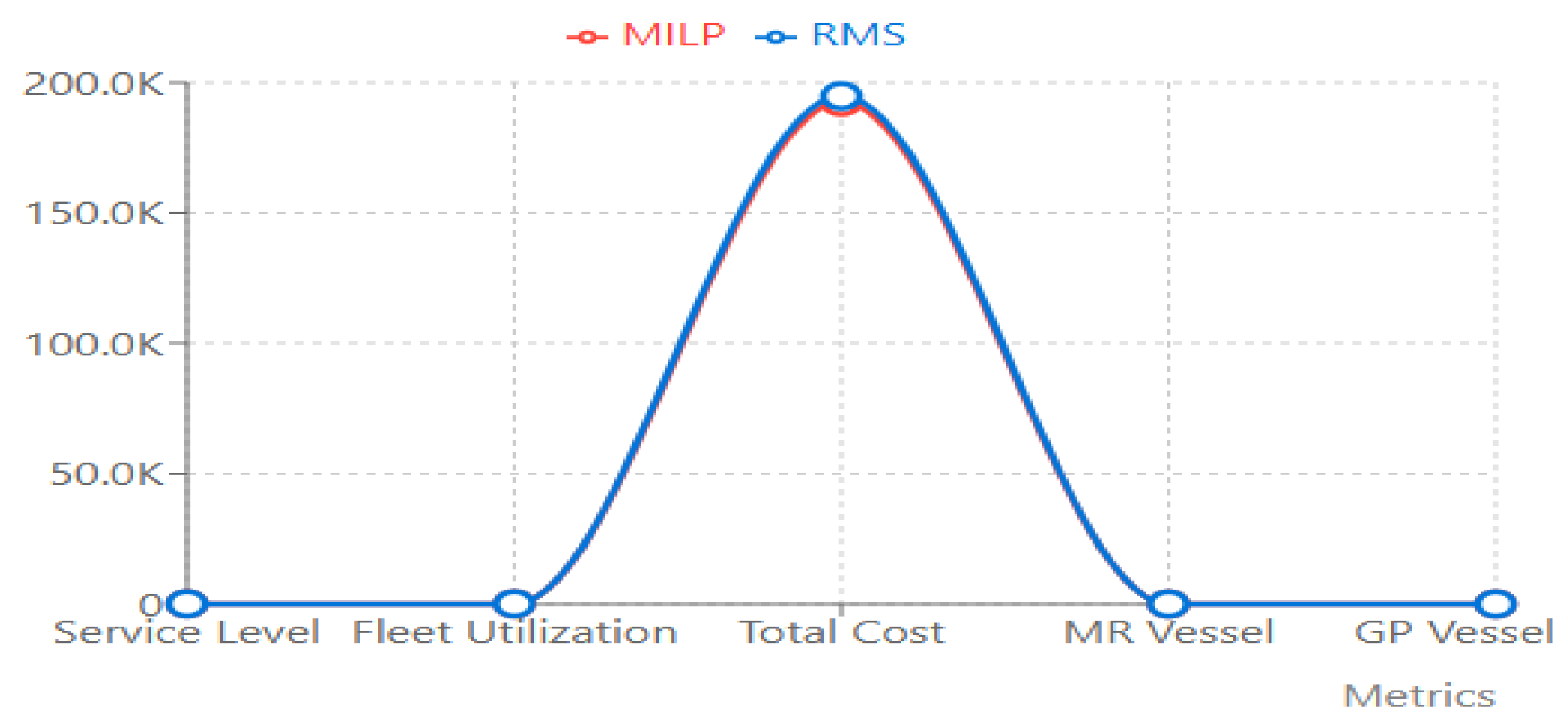
4.2.2. Comparing MILP and RSM
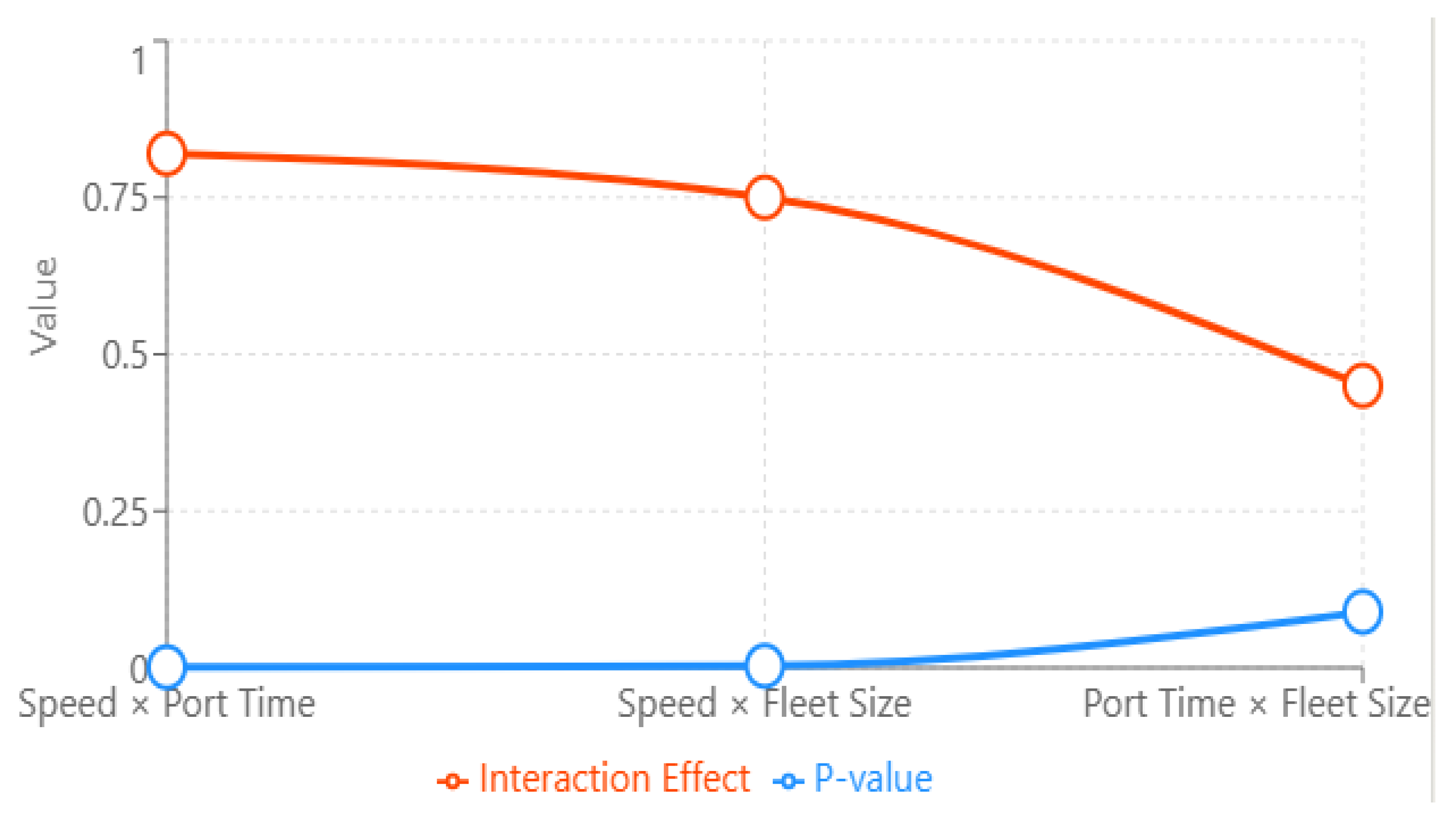
4.2.3. Significant Interaction Between Factors
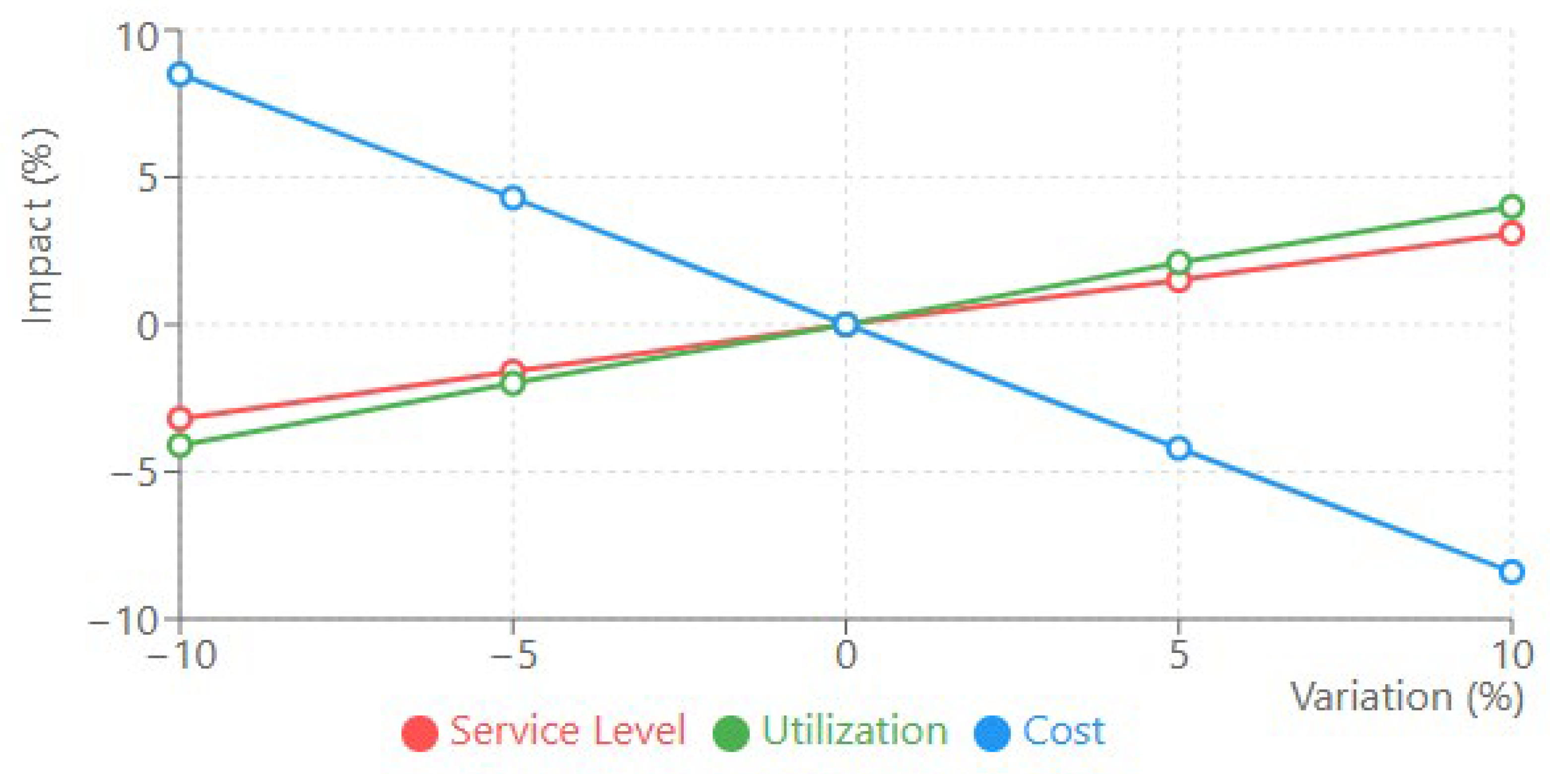
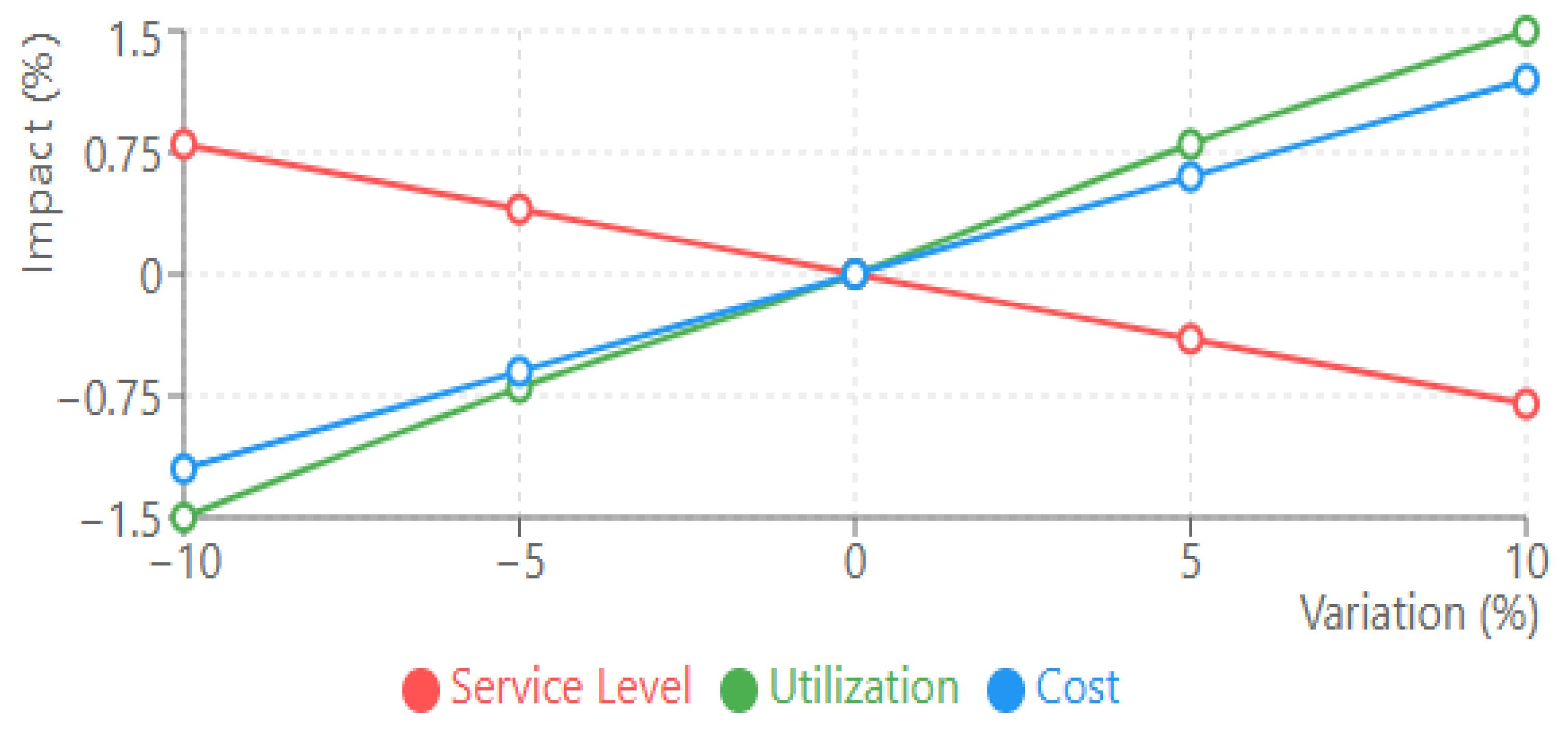
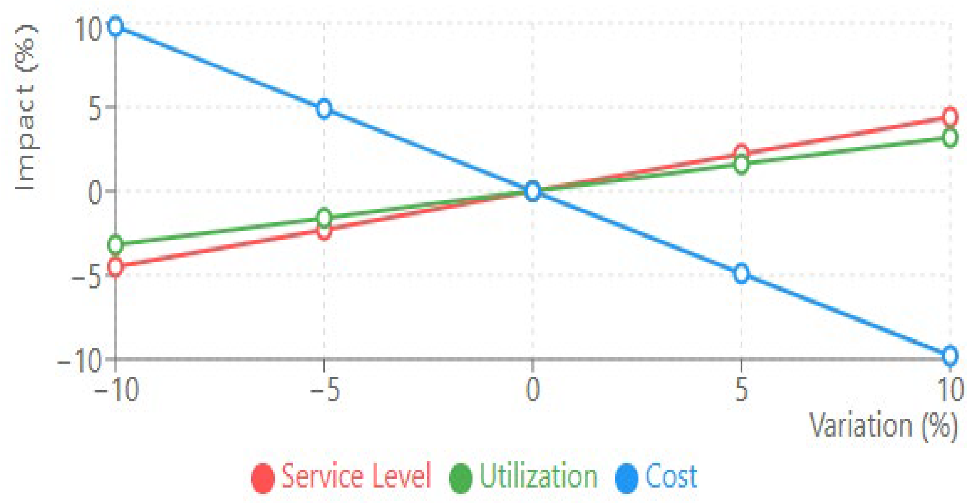
4.2.4. Sensitivity Analysis
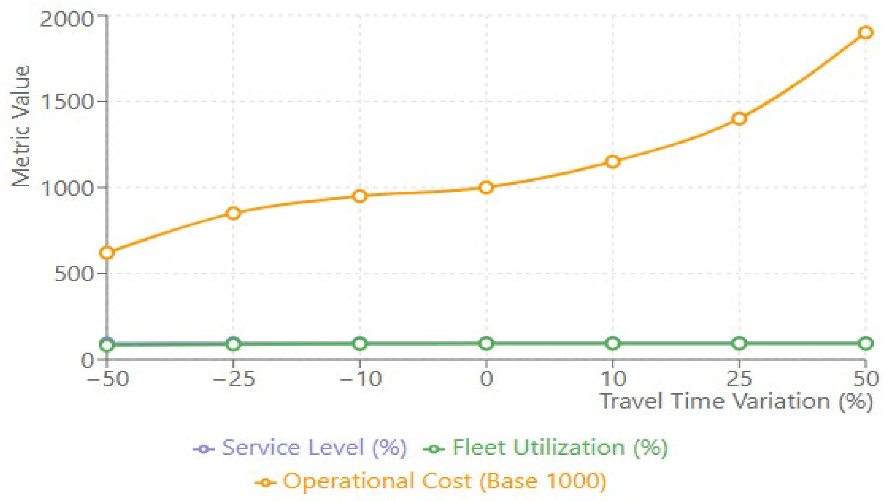
4.2.5. Travel Time Variations Impact
5. Discussion
6. Conclusions
6.1. Summary of Findings
6.2. Limitation and Future Work
6.2.1. Limitations
6.2.2. Future Research
- Optimization with Dynamics and Real-time
- 2.
- Enhanced Demand Modeling
- 3.
- Comprehensive Cost Modeling
Author Contributions
Funding
Data Availability Statement
Conflicts of Interest
References
- Afpriyanto, A.; Putra, I.N.; Jupriyanto, J.; Sari, P. Critical Role of Maritime Infrastructure in Indonesian Defense Logistics Management Towards the World Maritime Axis. Int. J. Humanit. Educ. Soc. Sci. Ijhess 2023, 1215–1224. [Google Scholar] [CrossRef]
- Lazuardi, S.D.; Riessen, B.V.; Achmadi, T.; Hadi, I.Z.; Mustakim, A. Analyzing the National Logistics System Through Integrated and Efficient Logistics Networks: A Case Study of Container Shipping Connectivity in Indonesia. Appl. Mech. Mater. 2017, 862, 238–243. [Google Scholar] [CrossRef]
- Panayides, P.M.; Borch, O.J.; Henk, A. Measurement Challenges of Supply Chain Performance in Complex Shipping Environments. Marit. Bus. Rev. 2018, 3, 431–448. [Google Scholar] [CrossRef]
- Barron, C.; Neis, P.; Zipf, A. A Comprehensive Framework for Intrinsic OpenStreetMap Quality Analysis. Trans. GIS 2013, 18, 877–895. [Google Scholar] [CrossRef]
- Freichel, S.L.; Rütten, P.; Wörtge, J.K. Challenges of Supply Chain Visibility in Distribution Logistics. Ekon. Vjesn. 2022, 35, 453–466. [Google Scholar] [CrossRef]
- Caridi, M.; Crippa, L.; Perego, A.; Sianesi, A.; Tumino, A. Measuring Visibility to Improve Supply Chain Performance: A Quantitative Approach. Benchmark. Int. J. 2010, 17, 593–615. [Google Scholar] [CrossRef]
- Soemanto, A. The Role of Oil Fuels on the Energy Transition Toward Net Zero Emissions in Indonesia: A Policy Review. Evergreen 2023, 10, 2074–2083. [Google Scholar] [CrossRef]
- Notteboom, T.; Pallis, A.A.; Rodrigue, J.-P. Disruptions and Resilience in Global Container Shipping and Ports: The COVID-19 Pandemic Versus the 2008–2009 Financial Crisis. Marit. Econ. Logist. 2021, 23, 179–210. [Google Scholar] [CrossRef]
- Handayani, D.I.; Masudin, I.; Rusdiansyah, A.; Suharsono, J. Production-Distribution Model Considering Traceability and Carbon Emission: A Case Study of the Indonesian Canned Fish Food Industry. Logistics 2021, 5, 59. [Google Scholar] [CrossRef]
- Azab, R.; Mahmoud, R.S.; Elbehery, R.; Gheith, M. A Bi-Objective Mixed-Integer Linear Programming Model for a Sustainable Agro-Food Supply Chain with Product Perishability and Environmental Considerations. Logistics 2023, 7, 46. [Google Scholar] [CrossRef]
- Busse, A.; Gerlach, B.; Lengeling, J.C.; Poschmann, P.; Werner, J.; Zarnitz, S. Towards Digital Twins of Multimodal Supply Chains. Logistics 2021, 5, 25. [Google Scholar] [CrossRef]
- Binsfeld, T.; Gerlach, B. Quantifying the Benefits of Digital Supply Chain Twins—A Simulation Study in Organic Food Supply Chains. Logistics 2022, 6, 46. [Google Scholar] [CrossRef]
- Gerlach, B.; Zarnitz, S.; Nitsche, B.; Straube, F. Digital Supply Chain Twins—Conceptual Clarification, Use Cases and Benefits. Logistics 2021, 5, 86. [Google Scholar] [CrossRef]
- Zhao, S.; Li, P.; Li, Q. The Vehicle Routing Problem Considering Customers’ Multiple Preferences in Last-Mile Delivery. Teh. Vjesn. Tech. Gaz. 2024, 31, 734–743. [Google Scholar] [CrossRef]
- Hu, Z.; Parwani, V.; Hu, G. Closed-Loop Supply Chain Network Design Under Uncertainties Using Fuzzy Decision Making. Logistics 2021, 5, 15. [Google Scholar] [CrossRef]
- Tehrani, M.; Gupta, S.M. Designing a Sustainable Green Closed-Loop Supply Chain Under Uncertainty and Various Capacity Levels. Logistics 2021, 5, 20. [Google Scholar] [CrossRef]
- Momeni, M.A. A Multi-Objective Model for Designing a Sustainable Closed-Loop Supply Chain Logistics Network. Logistics 2024, 8, 29. [Google Scholar] [CrossRef]
- Li, Z.; Zhang, Y.; Zhang, G. Two-Stage Stochastic Programming for the Refined Oil Secondary Distribution with Uncertain Demand and Limited Inventory Capacity. IEEE Access 2020, 8, 119487–119500. [Google Scholar] [CrossRef]
- Fu, M.; Wang, D. Evaluation of Crowdsourcing Logistics Service Quality Based on Entropy Weight Method and Analytic Hierarchy Process. E3S Web Conf. 2021, 257, 2082. [Google Scholar] [CrossRef]
- Cerdá, J.; Pautasso, P.C.; Cafaro, D.C. Optimizing Gasoline Recipes and Blending Operations Using Nonlinear Blend Models. Ind. Eng. Chem. Res. 2016, 55, 7782–7800. [Google Scholar] [CrossRef]
- Robles, J.O.; Azzaro-Pantel, C.; Aguilar-Lasserre, A.A. Optimization of a Hydrogen Supply Chain Network Design Under Demand Uncertainty by Multi-Objective Genetic Algorithms. Comput. Chem. Eng. 2020, 140, 106853. [Google Scholar] [CrossRef]
- Aldossary, M. Multi-Layer Fog-Cloud Architecture for Optimizing the Placement of IoT Applications in Smart Cities. Comput. Mater. Contin. 2023, 75, 633–649. [Google Scholar] [CrossRef]
- Setyawati, D.R.; Surini, S.; Mardliyati, E. Optimization of Luteolin-Loaded Transfersome Using Response Surface Methodology. Int. J. Appl. Pharm. 2017, 9, 107–111. [Google Scholar] [CrossRef] [PubMed]
- Chen, X.; Wang, W.; Li, S.; Xue, J.; Fan, L.; Sheng, Z.; Chen, Y. Optimization of Ultrasound-Assisted Extraction of Lingzhi Polysaccharides Using Response Surface Methodology and Its Inhibitory Effect on Cervical Cancer Cells. Carbohydr. Polym. 2010, 80, 944–948. [Google Scholar] [CrossRef]
- Wu, X.; Jiang, Y. Source-Network-Storage Joint Planning Considering Energy Storage Systems and Wind Power Integration. IEEE Access 2019, 7, 137330–137343. [Google Scholar] [CrossRef]
- Ekpu, M. Optimisation of a Microelectronic Assembly Package Using Response Surface Methodology. Niger. J. Technol. 2021, 39, 1058–1065. [Google Scholar] [CrossRef]
- Wang, H.; Zhang, Y.; Qin, S. A Study on Ductility of Prestressed Concrete Pier Based on Response Surface Methodology. Eng. Technol. Appl. Sci. Res. 2016, 6, 1253–1257. [Google Scholar] [CrossRef]
- Gao, H.; Xu, G.; Nan, H.; Kong, J.; Niu, S.; Zhao, X. Optimization of the Prescription of Pomelo Beverage by Response Surface Methodology. In Proceedings of the 2010 2nd International Conference on Information Engineering and Computer Science, Wuhan, China, 25–26 December 2010; pp. 1–3. [Google Scholar] [CrossRef]
- Yuan, C.; Liu, B.; Chen, Y.S.; Chen, Y.Z. Optimization of Preparation of Jujube Juice by Response Surface Methodology. Adv. Mater. Res. 2012, 455–456, 981–984. [Google Scholar] [CrossRef]

| Supply Port | Capacity | Oil Products | ||
|---|---|---|---|---|
| Gasoline | Diesel | Kerosene | ||
| DUM | 531,000 | 212,400 | 254,880 | 63,720 |
| PLJ | 402,000 | 253,260 | 100,500 | 48,240 |
| CLC | 996,000 | 288,000 | 372,000 | 336,000 |
| BLP | 1,139,100 | 243,000 | 386,100 | 510,000 |
| BAL | 375,000 | 243,750 | 131,250 | 0 |
| KSM | 18,771 | 5961 | 7317 | 5493 |
| Demand Port | Gasoline | Diesel | Kerosene |
|---|---|---|---|
| BLW | 22,715 | 14,455 | 4130 |
| TUB | 38,500 | 24,500 | 7000 |
| TGE | 18,375 | 8575 | 24,500 |
| SBY | 26,250 | 15,750 | 2450 |
| TBN | 87,500 | 52,500 | 0 |
| SMG | 27,685 | 11,865 | 0 |
| PSB | 63,000 | 26,250 | 15,750 |
| PJG | 105,035 | 57,764 | 31,773 |
| TKA | 22,050 | 8750 | 4200 |
| TPR | 149,296 | 67,424 | 24,080 |
| MGS | 10,878 | 21,224 | 4298 |
| TWA | 8750 | 5138 | 693 |
| WAY | 33,600 | 14,784 | 7392 |
| BBA | 21,000 | 9240 | 4620 |
| KOB | 31,500 | 13,860 | 6930 |
| MKS | 19,320 | 9660 | 3864 |
| KUP | 2499 | 1631 | 168 |
| PLP | 3689 | 1666 | 595 |
| BIT | 9240 | 4158 | 10,500 |
| Type of Vessel | Vessel Speed | Capacity Compartments | ||
|---|---|---|---|---|
| Gasoline | Diesel | Kerosene | ||
| GP | 13 Knot | 10,008 | 7149 | 7149 |
| MR | 14 Knot | 14,506 | 13,056 | 14,505 |
| Type of Vessel | Travel Cost (USD) | Port Cost (USD) | Penalty Cost (USD) |
|---|---|---|---|
| GP | 6752 | 223 | 7 |
| MR | 11,850 | 569 | 7 |
| 0 | 1 | 2 | 3 | 4 | 5 | 6 | 7 | 8 | 9 | 10 | 11 | 12 | 13 | 14 | 15 | 16 | 17 | 18 | 19 | 20 | 21 | 22 | 23 | 24 | 25 |
|---|---|---|---|---|---|---|---|---|---|---|---|---|---|---|---|---|---|---|---|---|---|---|---|---|---|
| 1 | 0 | 1.9 | 4.3 | 5.2 | 9.2 | 8.6 | 1.2 | 0.9 | 2.5 | 4 | 0.9 | 3.6 | 0.85 | 3 | 4.8 | 2.9 | 6.1 | 6 | 7.6 | 10.8 | 4.8 | 5.4 | 6.8 | 11.6 | 7 |
| 2 | 1.9 | 0 | 2.9 | 4.3 | 1.7 | 10 | 3.1 | 1.1 | 1.1 | 3.2 | 2.8 | 2.2 | 1.1 | 1.7 | 3.4 | 1.4 | 4.4 | 4.4 | 9.2 | 9.3 | 3.7 | 4.2 | 6.9 | 10.1 | 6.9 |
| 3 | 4.3 | 2.9 | 0 | 5.4 | 2 | 7.7 | 5.9 | 4 | 2.3 | 3.5 | 3.2 | 2.6 | 3.9 | 1.4 | 3.3 | 1.7 | 1.6 | 1.5 | 7.1 | 7 | 4.8 | 5.1 | 4.1 | 8 | 8 |
| 4 | 5.2 | 4.3 | 5.4 | 0 | 3.5 | 5.7 | 7.1 | 5.1 | 3.9 | 2.5 | 3.9 | 3.1 | 5.2 | 4.6 | 6.3 | 3.7 | 6.9 | 6.9 | 4.9 | 5 | 0.7 | 1.4 | 6.8 | 5.8 | 2.6 |
| 5 | 9.2 | 1.7 | 2 | 3.5 | 0 | 9.2 | 4.7 | 2.7 | 1 | 1.6 | 1.3 | 0.6 | 2.7 | 2.2 | 3.1 | 0.3 | 3.6 | 3.5 | 8.4 | 8.5 | 2.9 | 3.2 | 6.1 | 9.3 | 6.1 |
| 6 | 8.6 | 10 | 7.7 | 5.7 | 9.2 | 0 | 12.3 | 10.2 | 9.6 | 8.2 | 8.3 | 8.8 | 10.3 | 9.1 | 11 | 9.4 | 6.1 | 6.5 | 6.5 | 3.2 | 6.3 | 6.3 | 3.6 | 4 | 3 |
| 7 | 1.2 | 3.1 | 5.9 | 7.1 | 4.7 | 12.3 | 0 | 2.1 | 4.2 | 6.2 | 11 | 5.3 | 2 | 2.5 | 3.8 | 4.4 | 7.5 | 7.5 | 12 | 12.2 | 6.5 | 7.1 | 10 | 13 | 9.8 |
| 8 | 0.9 | 1.1 | 4 | 5.1 | 2.7 | 10.2 | 2.1 | 0 | 2.2 | 4.2 | 3.8 | 3.3 | 0.1 | 0.6 | 4.5 | 2.4 | 5.5 | 5.5 | 9.9 | 10.1 | 4.5 | 5.1 | 8 | 11 | 7.7 |
| 9 | 2.5 | 1.1 | 2.3 | 3.9 | 1 | 9.6 | 4.2 | 2.2 | 0 | 2.5 | 2.2 | 1.6 | 2.2 | 1.6 | 2.9 | 0.7 | 3.8 | 3.8 | 8.8 | 9 | 3.3 | 3.6 | 6.4 | 9.8 | 6.6 |
| 10 | 4 | 3.2 | 3.5 | 2.5 | 1.6 | 8.2 | 6.2 | 4.2 | 2.5 | 0 | 6.4 | 1.2 | 4.2 | 2.7 | 4.6 | 1.8 | 5.1 | 5.1 | 7.4 | 7.5 | 1.9 | 2.2 | 7.6 | 8.3 | 5.1 |
| 11 | 0.9 | 2.8 | 3.2 | 3.9 | 1.3 | 8.3 | 11 | 3.8 | 2.2 | 6.4 | 0 | 0.9 | 3.9 | 2.4 | 4.3 | 1.5 | 4.7 | 4.7 | 7.6 | 7.7 | 2 | 2.3 | 7.2 | 8.5 | 5.3 |
| 12 | 3.6 | 2.2 | 2.6 | 3.1 | 0.6 | 8.8 | 5.3 | 3.3 | 1.6 | 1.2 | 0.9 | 0 | 3.3 | 1.8 | 3.7 | 0.9 | 4.1 | 4.1 | 8.1 | 8.2 | 2.5 | 2.8 | 6.6 | 9 | 5.8 |
| 13 | 0.85 | 1.1 | 3.9 | 5.2 | 2.7 | 10.3 | 2 | 0.1 | 2.2 | 4.2 | 3.9 | 3.3 | 0 | 2.8 | 4.5 | 2.4 | 5.5 | 5.5 | 10 | 10.2 | 4.5 | 5.1 | 8 | 11 | 7.8 |
| 14 | 3 | 1.7 | 1.4 | 4.6 | 2.2 | 9.1 | 2.5 | 0.6 | 1.6 | 2.7 | 2.4 | 1.8 | 2.8 | 0 | 2.1 | 0.9 | 2.9 | 2.9 | 8.5 | 8.4 | 3.9 | 4.2 | 5.4 | 9.4 | 7.2 |
| 15 | 4.8 | 3.4 | 3.3 | 6.3 | 3.1 | 11 | 3.8 | 4.5 | 2.9 | 4.6 | 4.3 | 3.7 | 4.5 | 2.1 | 0 | 2.8 | 4.9 | 4.8 | 10.4 | 10.3 | 5.7 | 6 | 7.4 | 11.3 | 8.9 |
| 16 | 2.9 | 1.4 | 1.7 | 3.7 | 0.3 | 9.4 | 4.4 | 2.4 | 0.7 | 1.8 | 1.5 | 0.9 | 2.4 | 0.9 | 2.8 | 0 | 3.3 | 3.2 | 8.6 | 8.7 | 3.1 | 3.4 | 5.8 | 9.5 | 6.3 |
| 17 | 6.1 | 4.4 | 1.6 | 6.9 | 3.6 | 6.1 | 7.5 | 5.5 | 3.8 | 5.1 | 4.7 | 4.1 | 5.5 | 2.9 | 4.9 | 3.3 | 0 | 0.4 | 5.6 | 5.4 | 6.3 | 6.6 | 2.5 | 6.4 | 6.7 |
| 18 | 6 | 4.4 | 1.5 | 6.9 | 3.5 | 6.5 | 7.5 | 5.5 | 3.8 | 5.1 | 4.7 | 4.1 | 5.5 | 2.9 | 4.8 | 3.2 | 0.4 | 0 | 5.9 | 5.8 | 6.3 | 6.6 | 2.9 | 6.8 | 7 |
| 19 | 7.6 | 9.2 | 7.1 | 4.9 | 8.4 | 6.5 | 12 | 9.9 | 8.8 | 7.4 | 7.6 | 8.1 | 10 | 8.5 | 10.4 | 8.6 | 5.6 | 5.9 | 0 | 2.4 | 5.6 | 5.6 | 3 | 3.4 | 2.3 |
| 20 | 10.8 | 9.3 | 7 | 5 | 8.5 | 3.2 | 12.2 | 10.1 | 9 | 7.5 | 7.7 | 8.2 | 10.2 | 8.4 | 10.3 | 8.7 | 5.4 | 5.8 | 2.4 | 0 | 5.7 | 5.7 | 2.9 | 1.4 | 2.4 |
| 21 | 4.8 | 3.7 | 4.8 | 0.7 | 2.9 | 6.3 | 6.5 | 4.5 | 3.3 | 1.9 | 2 | 2.5 | 4.5 | 3.9 | 5.7 | 3.1 | 6.3 | 6.3 | 5.6 | 5.7 | 0 | 1.1 | 7.5 | 6.5 | 3.3 |
| 22 | 5.4 | 4.2 | 5.1 | 1.4 | 3.2 | 6.3 | 7.1 | 5.1 | 3.6 | 2.2 | 2.3 | 2.8 | 5.1 | 4.2 | 6 | 3.4 | 6.6 | 6.6 | 5.6 | 5.7 | 1.1 | 0 | 7.5 | 6.5 | 3.3 |
| 23 | 6.8 | 6.9 | 4.1 | 6.8 | 6.1 | 3.6 | 10 | 8 | 6.4 | 7.6 | 7.2 | 6.6 | 8 | 5.4 | 7.4 | 5.8 | 2.5 | 2.9 | 3 | 2.9 | 7.5 | 7.5 | 0 | 3.9 | 4.2 |
| 24 | 11.6 | 10.1 | 8 | 5.8 | 9.3 | 4 | 13 | 11 | 9.8 | 8.3 | 8.5 | 9 | 11 | 9.4 | 11.3 | 9.5 | 6.4 | 6.8 | 3.4 | 1.4 | 6.5 | 6.5 | 3.9 | 0 | 3.2 |
| 25 | 7 | 6.9 | 8 | 2.6 | 6.1 | 3 | 9.8 | 7.7 | 6.6 | 5.1 | 5.3 | 5.8 | 7.8 | 7.2 | 8.9 | 6.3 | 6.7 | 7 | 2.3 | 2.4 | 3.3 | 3.3 | 4.2 | 3.2 | 0 |
| Factor | Range | Respond |
|---|---|---|
| Vessel Speed | 10–15 | Service level |
| Port Time | 0.3–0.7 | Cost |
| Fleet Size | 20–35 | Fleet Utilization |
| Routes | Vessel | Trip | Days | Utilization | Total Cost/Month | Load Factor | |
|---|---|---|---|---|---|---|---|
| Western Cluster | DUM-TUB-PSB | MR | 5 | 20 | |||
| PLJ-TPR | MR | 6 | 19.2 | ||||
| BAL-PJG | MR | 4 | 20.8 | ||||
| BAL-TGE-TKA | GP | 6 | 36 | ||||
| DUM-BLW | GP | 4 | 11.2 | ||||
| 92.3% | USD 1,284,250 | 88.4% | |||||
| Central Cluster | CLC-TBN | MR | 4 | 28.8 | |||
| CLC-SMG-SBY | MR | 3 | 25.8 | ||||
| BLP-KOB-MKS | GP | 5 | 30 | ||||
| BLP-MGS-TWA | GP | 4 | 28.8 | ||||
| 89.7% | USD 892,460 | 91.2% | |||||
| Eastern Cluster | KSM-BIT-WAY | GP | 6 | 72.6 | |||
| BLP-BBA | GP | 3 | 21.6 | ||||
| BLP-KUP-PLP | GP | 2 | 26.2 | ||||
| 87.5% | USD 638,946 | 85.7% | |||||
| Total | MR = 13 GP = 15 28 | $2,815,926 |
| Metrics | MILP | RMS | Differences | % Variance |
|---|---|---|---|---|
| Service level | 97.2% | 92.2% | −0.4% | −0.41% |
| Fleet Utilization | 85.5% | 86.2% | +0.7% | +0.82 |
| Total Cost | 192,500 | 194,800 | +2300 | +1.19% |
| MR Vessel | 13 | 13 | 0 | 0% |
| GP Vessel | 15 | 15 | 0 | 0% |
Disclaimer/Publisher’s Note: The statements, opinions and data contained in all publications are solely those of the individual author(s) and contributor(s) and not of MDPI and/or the editor(s). MDPI and/or the editor(s) disclaim responsibility for any injury to people or property resulting from any ideas, methods, instructions or products referred to in the content. |
© 2025 by the authors. Licensee MDPI, Basel, Switzerland. This article is an open access article distributed under the terms and conditions of the Creative Commons Attribution (CC BY) license (https://creativecommons.org/licenses/by/4.0/).
Share and Cite
Sirait, M.; Charnsethikul, P.; Paoprasert, N. A Multi-Type Ship Allocation and Routing Model for Multi-Product Oil Distribution in Indonesia with Inventory and Cost Minimization Considerations: A Mixed-Integer Linear Programming Approach. Logistics 2025, 9, 35. https://doi.org/10.3390/logistics9010035
Sirait M, Charnsethikul P, Paoprasert N. A Multi-Type Ship Allocation and Routing Model for Multi-Product Oil Distribution in Indonesia with Inventory and Cost Minimization Considerations: A Mixed-Integer Linear Programming Approach. Logistics. 2025; 9(1):35. https://doi.org/10.3390/logistics9010035
Chicago/Turabian StyleSirait, Marudut, Peerayuth Charnsethikul, and Naraphorn Paoprasert. 2025. "A Multi-Type Ship Allocation and Routing Model for Multi-Product Oil Distribution in Indonesia with Inventory and Cost Minimization Considerations: A Mixed-Integer Linear Programming Approach" Logistics 9, no. 1: 35. https://doi.org/10.3390/logistics9010035
APA StyleSirait, M., Charnsethikul, P., & Paoprasert, N. (2025). A Multi-Type Ship Allocation and Routing Model for Multi-Product Oil Distribution in Indonesia with Inventory and Cost Minimization Considerations: A Mixed-Integer Linear Programming Approach. Logistics, 9(1), 35. https://doi.org/10.3390/logistics9010035