1. Introduction
With the development of technology, customers are becoming more and more dependent on electronic products. The flood of electronic products brings about a prominent e-waste problem. Therefore, governments have introduced production recycling legislation, and manufacturers have developed production recovery programs to seek business opportunities from remanufactured products. Therefore, customers benefit from the use of good quality products at a lower price. In the last few decades, researchers have defined “remanufacturing” in different ways. Johnson and McCarthy define “remanufacturing” as a rebuilding process from the original manufactured product to a combination of reused, repaired, and new parts [
1]. Thierry, Salomon, Van Numen, and Van Wassenhove explain that remanufacturing brings used products up to the same quality standards as those for new products and can be combined with technological upgrading [
2]. The Remanufacturing Industrial Council put more emphasis on remanufactured products being returned to a “like-new” or “better-than-new” condition, and warranted with regard to performance level and quality [
3]. Scientists have also shed light in the area of remanufacturing. Gungor and Gupta report a survey on the issues in environmentally conscious manufacturing and product recovery (ECMPRO) [
4]. They highlight the elements of environmentally conscious remanufacturing and the recovery of materials and products, including lifecycle analysis and design, assembling and dissembling, inventory control, and production planning. Ten years later, Ilgin and Gupta developed a framework and extended environmentally conscious product design to reverse and closed-loop supply chains [
5]. They also introduced the new topic of marketing for remanufactured products. Researchers consider the environment, the economy, the customer, and the material requirement simultaneously to help government, the manufacturer, and the customer achieve their goals.
In the past, scientists have often focused on remanufacturing durable goods, such as home appliances, motor vehicle parts, and medical equipment [
6,
7]. Durable goods were believed to have more residual value after acquisition [
8]. Unused value can be extracted from acquired products through remanufacturing operations. Only a few scientists have conducted studies on the remanufacturing of short-lifecycle products, such as consumer goods in the apparel industry and the high-technology electronics industry [
9]. Gan, Pujawan, and Suparno established three categories in the remanufacturing of short lifecycle products: product characteristics, demand-related factors, and supply-related factors [
10]. The major differences between durable goods and short lifecycle goods include the customers’ duration of usage and the remaining value after disposal. However, the essence of this difference does not originate from intrinsic product quality and reliability, but the specific circumstances around short-lifecycle products. For instance, products in the apparel industry fade seasonally because of changes in fashion behavior. Electronic products are outdated because of innovation and shifts in lifestyle. Nowadays, high-technology companies introduce new generations of products frequently to maintain customers’ interest. The smartphone industry is a case in point. Products are retired after about 18 months on average in America [
11]. Customers always crave the newest generation and upgrade their products for social needs because the latest features are often based on the latest technology [
11]. Therefore, high-technology products have two different properties: an intrinsic function and social compatibility. Customers have different tolerance levels for the two properties. If one of the properties depreciates below a certain threshold, the customer will stop using the product. High-technology products are classified as short-lifecycle products because they cannot satisfy customers’ fast-changing and innovative social needs, and not because they cannot maintain reliability in use. Remanufacturing operations mitigate the obsolescence of the first property, while technology upgrading is key for the second one. Therefore, remanufacturing and upgrading end-of-use products are necessary to extract the remaining value from, and add social value to, used items, extending the lifespan of remanufactured high-technology products. The two operations cooperate to satisfy the appetite of those technology-sensitive customers who are also price-sensitive.
High-technology companies release new-generation products at an intensive rate. Newer models are often launched before older models are sold out. It is a common phenomenon that unsold new products belonging to the earlier generations remain in inventory when remanufactured items belonging to the later generations are available. However, remanufactured goods are in short supply because of the limited quantity of qualified end-of-use cores. Traditionally, the manufacturer only collects end-of-use products for remanufacturing and upgrading. However, the uncertainty in supply and demand [
12,
13,
14,
15], the quality of collected cores [
16], and the capacity for remanufacturing [
17] remain a challenge for remanufacturing operations. With respect to uncertainty in the quality of collected cores, used products returned from customers are not all remanufacturable, since some of them have no remaining value. Most of the qualified returns that are suitable for remanufacturing are typically business-to-business commercial returns [
10]. Compared to collected end-of-use products, an unsold new product has more value remaining in the first property. The quality is high and the product is reliable, as it has not been used. The timing of the return and the supply are controllable if the retailer and the manufacturer/remanufacturer have a good supply and customer relationship. Compared with recently released new products, the unsold and outdated new products become more and more unattractive with the development of new technology. Returning unsold products for upgrading becomes a possible better acquisition strategy. Upgraded products are more attractive technologically and can help to mitigate the short of supply of remanufactured products and reduce the holding cost of a slow seller. However, this solution decreases the customer’s perceived value due to the refurbishment process but increases the cost due to the reverse supply chain and the upgrading operations. Should a retailer keep selling outdated new products and target the new product market or return unsold products for upgrading and target the remanufactured market? For profit maximization purposes, it depends on the revenue, which is driven by demands for different types of products as well as selling prices, and on costs, including acquisition, remanufacturing, and upgrading costs. The new business model should consider all of the parties in the supply chain, such as the manufacturer, the collector, the remanufacturer, and retailer. Price sensitivity in customer segments, the perceived quality of remanufactured products, and the technology gap between generations can all influence the demand for different products, and, as a result, influence the manufacturer’s and retailer’s decision-making process on the price and acquisition strategy.
To the best of our knowledge, no study has paid attention to how customers’ attitudes towards quality and difference in generation, and products’ conditions in terms of quality and technology level, influence the selling prices and acquisition strategies for new and remanufactured high-technology products across generations. In addition to this, no scientists have studied the return of new products that belong to earlier generations for upgrading. The primary goal of this paper is to build profit maximization models in manufacturer, retailer, and joint supply chain scenarios for high-technology consumer products, such as laptops and smartphones, to help manufacturers and retailers determine the prices for new products that belong to out-of-date technology and remanufactured products that belong to the latest generation. Two acquisition strategies are examined: collect used products only, and acquire both used products and unsold new products. The retailer-collect model and the remanufacturer-collect model are compared. The optimal quantity of used products belonging to different generations and the optimal number of unsold new products to return are obtained in both models for all scenarios. In the next section, a literature review on acquisition strategies, pricing decisions on remanufactured short-lifecycle products, customers’ choices, the integration of pricing and planning, and product upgrade will be provided. Then, a detailed problem statement will be elicited. The model and the data resources will be examined in
Section 4 and
Section 5, respectively. The results are provided in
Section 6. Conclusions and future research directions will be given in
Section 7.
2. Literature Review
This study is related to three research points. First, the study focuses on pricing decisions for new and remanufactured short-lifecycle products. Price models from previous research are presented. Second, the research is about a new acquisition strategy for recycling end-of-use and overstock high-technology products. Related papers about reverse supply chain are reviewed. Third, the paper relates to remanufacturing of high technology products. Former studies are examined to obtain remanufacturing strategies.
2.1. Price Decisions for Short Lifecycle Products
To determine the selling price, the demand function is important. Bass created the well-known Bass model for consumer durables based on the parameters of innovation and imitation [
18]. Then Norton and Bass extended the Bass model to three production generations and applied the theory to hi-tech products [
19]. Wang and Tung created a time-dependent diffusion demand model with different discount levevls to determine the optimal order quantity and selling prices for gradually outdating products [
20]. Then Gan, Pujawan, Suparno and Widodo developed and applied the model to new and remanufactured products with a short lifecycle [
21]. They found that decreasing the price of the new product during the demand decrease phase was not profitable for the whole supply chain system. Later, Zhou, Gupta, Knoshita and Yamada extended the model to determine prices for new and remanufactured products across generations [
22]. Pricing strategy is discussed with respect to the period when new products belonging to the earlier generation and the remanufactured product belonging to the latest generation are in the same market simultaneously. They found that increasing the price of the newly launched product increases the price differentiation between new and remanufactured products belonging to different generations. The studies discussed above build on models based on linear demand functions. However, Li and Huh examine a nonlinear price-sensitive model to find the optimal set of discrete prices with limited times of price changes, catering to customer demand as it varies over time [
23].
Price is a sensitive factor for the revenue in an organization, and is driven by cost, inventory, time, customers’ willingness to pay, government regulation, and even competitors. Separating price from other factors is impossible in the real world. The customer is critical to pricing. Learning the customer’s perceived value for remanufactured products and technology expectations is essential to making a decision. Empirical studies show that remanufactured products’ attractiveness is highly influenced by price discount and brand equity for high-technology products. However, brand equity is less important than quality [
24]. The other potential impact factor is the product technology selection. More customers concentrate on technology development; the newer the technology, the higher the market potential [
25].
The supply of remanufactured products is restricted by the number of goods and parts that are returned. The demand curve can be linear or nonlinear, deterministic or probabilistic, and varies by customer segment, time, and price. The demand is always uncertain. For remanufactured products, keeping the balance between supply and demand is key to success. Inventory study is a way to control supply–demand balance. Vadde, Kamarthi and Zeid built a pricing model for remanufactured products under stochastic demand in the environment of inventory fluctuations [
26]. Then Vadde, Kamarthi and Gupta conducted another related study and focused on inventory imbalance between the arrival rates of discarded products and the demand trend [
27]. They looked at disposal decisions based on pricing policies to achieve minimization of inventory fluctuations. They established a stochastic dynamic programming model and found that it was better to dispose of product when the carrying cost exceeds the disposal cost. Different from the stochastic model, Gupta summarized decentralized and centralized deterministic models, integrating the inventory level, pricing and return reimbursements in a JIT environment [
28]. The study included various scenarios, including a decentralized model with a wholesale price set by the market, a decentralized model with a wholesale price set by the manufacturer, and a centralized model for supply chain optimality. Akan, Ata and Savaskan-Ebertk built a dynamic pricing model with a life cycle considered for remanufacturable products in order to retain the balance between supply and demand [
29]. They integrated optimal pricing, production and inventory policies in the problem model, including the timing of launching remanufactured products, co-existence strategy with new products, remanufacturing cost benefit, attractiveness, and return rate. They recognize the conflict between selling more new products and the increase in the user pool for remanufacturing and charging more to protect value depreciation. If the remanufactured product is offered side-by-side with the new product, remanufacturing cost, attractiveness, and product return rate are critical for its survival. Kwak and Kim presented a multi-objective model to maximize the profit and minimize the environmental impact for a line of new and remanufactured products by mixing the buyback prices, the selling prices, and the production plans together [
30]. Mixed-integer programming was used to optimize the profit. A transition matrix was used to coordinate pricing and production planning. However, the paper assumed no upgrade for remanufacturing, and considered a single period of a single generation with no competitor.
2.2. Reverse Supply Chain for Remanufactured Products
The majority of supplies of remanufactured products are from recycled parts. Therefore, a reverse supply chain strategy, including recovery method, recycle policy, and acquisition price, is critical to the availability of remanufactured products. Gan, Pujanan, Suparno take three recovery options into account, including component remanufacturing and product remanufacturing [
10]. They determine the options based on different types of returns, such as B2B or consumer returns, end of use or end of life returns.
More papers have focused on recycling policy for remanufacturing. Some of them keep an eye on the question of which party should collect used cores and how they should cooperate with each other. Savaskan, Bhattacharya, and Van Wassenhove conducted a study under the condition that the manufacturer was the Stackelberg leader. They compared three ways of collecting used cores: the manufacturer collects them directly, the retailer collects them, or a third party acquires them. They believe the retailer is the most effective undertaker, because it is closer to customers [
31]. Some studies explore optimal recycle channels. Zhao, Wei, and Li compare two models where a manufacturer adopts single-channel collection or dual-channel collection with a third party [
32]. Similar to Savaskan, Bhattacharya, and Van [
31], they suggest that the retailer engage in acquiring used cores regardless of the application of a single-channel model or a dual-channel model. Govindan and Popiuc build two reverse supply chain coordination models for the personal computers industry with the function of defining customer willingness to return obsolete products. The retailer collects the used cores for the manufacturer directly in the first model, and then a distributor is added in the middle, resulting in a three-echelon reverse supply chain. The results show that both models improve profits through coordination with revenue sharing contracts [
33]. Taleizadeh, Moshtagh, and Moon extend the research problem from a reverse supply chain to a closed-loop supply chain [
34]. They compare the single-channel forward with dual-channel reverse, dual-channel forward with dual-channel reverse with a game theoretical method, concluding that the second model brings greater benefit to the manufacturer.
As described in the Introduction section, the uncertainty of demand-supply and quality of used cores is a challenge in remanufacturing. Except for collection channel selection, using price levers to control uncertainties is the most popular mechanism [
12,
13,
14,
16]. Two papers we reviewed explore the relationship between acquisition and new product demand curves [
35,
36]. Both consider imitation and innovation factors in the new product demand function. One of them is focused on the optimal component reuse volume corresponding to acquisition costs [
35]. The authors try to determine how many end-of-life products should be collected, and their relationship with the new product diffusion demand curve, especially the condition when the return rate is high enough that intersects with new product sales. The other one is about acquisition methods, including trade-in and buyback. Cole, Mahapatra, and Webster compare the trade-in and the buyback policies for acquiring used product for remanufacturing in different conditions with myopic and proactive pricing algorithms, respectively [
36]. They find that the optimal policy is correlated with the time lag between the introduction of a new product and the initial demand for a remanufactured version. Another study develops an environmental sustainability economic order quantity (EOQ) model from the classical EOQ model, and considers the uncertainty of both market demand and acquisition quantity in a remanufacturing system [
37]. The authors aimed to minimize the inventory cost, maximize the environmental benefit, and coordinate forward and reverse logistics in a remanufacturing model. They confirm that replenishment of new items is vital to reducing the risk of shortage. Another paper points out that the challenges are not only the imbalance of demand and supply, but also a lack of planning, information, quality management, inventory management, remanufacturing processes, and automation [
38]. The authors use a series of lean tools such as standard operations, continuous flow, Kanban, and teamwork to project a reduction of 83–99 percent for lead time.
The purpose of remanufacturing is to reduce the environmental burden and create a business opportunity. Therefore, it is necessary to consider environment, economy, and customer benefit together. Turki, Sauvey, and Rezg take remanufacturing planning, differences in products, machine failures, carbon constraints, and customer demands into account in a discrete flow model [
39]. They find that set-up cost, the return rate of used items, and machine availability significantly influence storage and production planning of new and remanufactured products. The trading prices under the conditions of lower carbon and higher carbon are also exhibited.
2.3. Remanufacturing Strategy for Short Lifecycle Products
Remanufacturing strategy for high-technology products always considers the special state of the market whereby models from multiple product generations exist simultaneously. Bhattacharya, Guide, and Van Wassenhove propose a study on remanufacturing across new product generations focusing on optimal order quantities [
40]. They optimize the retailer’s profit in four different channels of decision-making structures, using the newsvendor model to determine the optimal order quantities from a manufacturer for the new products and the optimal order quantities from a remanufacturer using returned and unsold product from an earlier generation. The authors do not take the quality of used items and production design into account. Galbreth et al. fill this gap [
41]. They integrate the cost of disposal, innovation rate, and inferior quality rate into the model with the inverse demand function, and explain the product innovation trade-offs among the higher demand of the new product, higher disposal cost, and higher cost of upgrading. They also indicate a counter-intuitive finding that increasing the cost of designing reusable products is an incentive for reuse.
Product generation development causes rapid technology depreciation. Researchers have a common understanding that remanufacturing, along with technological upgrading, is a way to maintain market competitiveness for remanufactured products. Galbreth, Boyaci and Verter analyze and compare the three models of no reusability, remanufacturing only, and remanufacturing while upgrading in terms of production cost, end-of-life cost, customer’s perceived value, and innovation rate and risk [
41]. Kwak and Kim provide a market positioning problem for remanufactured product combined with optimal planning for part upgrades while paying attention to the influence of production design in a waste-stream system and a market-driven system [
30]. This study aims to maximize remanufacturing profit and find optimal remanufacturing options, selling price, and production quantity using the concept of generational difference. The demand is determined by generational differences, selling price, and product status, using the techniques of discrete choice analysis and conjoint analysis. Recently, Khan, Mittal, West, and Wuest published a survey paper to investigate the concept of upgradability for extending product lifespan [
42]. They indicate the importance of Product-Service Systems (PPS) and the implementation of the circular economy.
Some papers have looked at the window of competition between the original equipment manufacturer (OEM) and the third-party manufacturer (TPM), should the TPM decide to take over remanufacturing operations [
15,
43,
44,
45,
46]. Atasu, Sarvary, and Van Wassenhove examine the competition effect on the aspect of demand for new and remanufactured products with green segments and product lifecycle [
43]. Subramanian, Ferguson, and Toktay take remanufacturing policies of high-end and low-end products into account [
44]. They find a negative effect on profit if the OEM and TPM take up remanufacturing operations simultaneously. Instead of third-party competition, looking for cooperation opportunities is another way to achieve a win-win outcome. Liu, Lei, Huang, and Leong examine the refurbishing authorization strategies for OEMs who produce electrical and electronic products [
45]. The results show that OEMs should consider a strategy of charging a lower fee when the customers are largely indifferent to remanufactured versus new products. Agrawal, Atasu, and Ittersum point out that sales cannibalization between new and remanufactured products does exist, but can be minimized by setting a higher price for the new ones. Remanufactured products can also be classified as manufacturer-refurbished and third-party refurbished. Third-party remanufactured products can differentiate the market of new products, giving rise to less influence on the part of new products [
46]. In addition, Huang and Wang are focused on how high a technology licensing fee the TPM should be charged [
15]. They suggest a higher fee when demand and supply is sufficient.
For a study regarding pricing, making decisions based on an appropriate demand function is important. The demand curves for high-technology products fit linear diffusion models well. For the discrete nonlinear model, the customer’s perceived value on quality and technology development are the keys to be determined. However, the price cannot be decided without considering the reverse supply chain and remanufacturing strategy. Undertaking recycling and reverse supply chain channel selection are popular research areas. To control the quantity and quality of returned cores, finding an optimal channel to recycle and using appropriate price levels are important. Trade-in policy is essential for future studies. To maintain the supply–demand balance, new parts are used if the supply of used cores is insufficient [
19]. Moreover, remanufacturing for high-technology products needs to overcome fast technology depreciation. Upgrading or remanufacturing to the original specification depends on product design, level of innovation, quality, reuse and disposal cost, and customer preference.
Most researchers have focused on remanufacturing only, without considering the generation effect on the short life cycle of products; some papers indicate the innovation impact on remanufacturing; even fewer consider how to deal with the unsold outdated product, but almost none talk about the pricing and acquisition decisions for unsold obsolete products and upgraded remanufactured products when they are competing in the same market. Many papers point out the profitability of the remanufactured product. However, the supply of the remanufactured products is restricted by the returned cores. The imbalance of supply and demand for the remanufactured products complicates the pricing and acquisition problem. As described above, returning a number of unsold products with a buyback price for upgrading and reselling is a possible solution to this issue. How to price unsold new products and remanufactured products, how many unsold new products should be returned for remanufacturing, and how many used units of each generation should be collected are within the scope of this paper.
This study will compare two models. The benchmark model uses the acquisition approach that only recycles end-of-use products belonging to different generations from customers. The developed model is based on the strategy that acquires end-of-use products and buybacks unsold new products from earlier generations as well. In the two models, manufacturer and retailer will act as the recycler, respectively. The results are compared, and an optimal strategy is determined.
3. Problem Statement
In this study, three types of products are defined.
Type 1: New products belonging to an earlier generation
Type 2: Upgraded remanufactured products belonging to the latest technology
Type 3: Recently released new products with the newest design and latest technology.
If a newer model is introduced, the previous one becomes unattractive. Customers are eager for the new technology. In a similar way, for the market of remanufactured products, upgraded remanufactured products are more welcome than those remanufactured to the original specification. When the OEM releases a new model, the previously unsold Type 3 products immediately become Type 1 products. The technology of newly produced Type 2 products is always at the highest level. The study assumes that Type 1 products have perfect product quality but outdated technology, while Type 2 products have quality inferior from the customers’ prospective, but the newest technology. The supply of Type 2 products comes from end-of-use products of previous generations from customers or unsold outdated new products returned by retailers. Customers who buy Type 1 or Type 2 products are in the middle level, differentiated from the customers who purchase brand new released models (Type 3). Therefore, the market of Type 1 and Type 2 products is assumed to be separate from the market of Type 3 products. Additionally, the demand for the upgraded remanufactured product is considerable and exceeds the supply from the end-of-use products. Type 1 products could be returned for an upgrade and sold as a Type 2 product. Only Type 1 and Type 2 products are within the scope of this study.
Three parties are in the system. They are the manufacturer, the remanufacturer, and the retailer. The OEM produces the new products belonging to the latest technology. The retailer sells the newest and the second newest models. The remanufacturer or the retailer collects the pre-owned products from customers at an acquisition price based on the product generation. It is assumed that only qualified items are acceptable. As described in the introduction, based on a consumer’s purchase behavior, smartphones are retired much earlier than their end-of-life; most acquired used products are end-of-use products; end-of-life products are not considered in the model. The manufacturer can also buy back unsold Type 1 products from the retailer at a buyback price. Two acquisition strategies are analyzed and compared. The first strategy is to acquire end-of-use products only for remanufacturing and upgrading. Unsold Type 1 products are not allowed to be returned. They have to be sold by retailers, and are in competition with recently released new products and upgraded remanufactured products. The second policy is to collect end-of-use products from customers for remanufacturing and upgrading, and buy back an optimal quantity of unsold Type 1 products from the retailer for upgrading. The rest of the Type 1 products are also available for sale. The system is presented in
Figure 1. Both remanufacturer and retailer are eligible to acquire used products from consumers. However, the optimal undertaker of acquisition should be identified. The retailer-recycle and remanufacturer-recycle models are built and compared in each acquisition strategy.
Assume a new product model is released every year. Profit maximizing models are built during a single time period of half a year after the newest model is launched. The revenue comes from selling Type 1 and Type 2 products during the period after the latest generation is released. Customers’ purchase decisions are based on three factors: product quality, price, and generation. A fixed fraction α of customers will return used products. The remanufacturer accepts all the items returned. In a future study, it would be easy to add a stochastic yield function if the quality acceptance level needs to be considered. Lead time is ignored. Customers are asked to order early. A stochastic function can be added in the model if the lead time is expected to be considered. The manufacturer follows the make-to-order policy. Remanufacturing cannot change the external features, parts can only be replaced or upgraded. The upgrade technology barrier is not considered. Production level is also ignored, as both manufacturer and remanufacturer have sufficient capacity to maintain good deliveries. The costs include manufacturing, remanufacturing, buy-back acquisition, upgrading, shortage, and inventory holding. Remanufacturing a product from the previous generation is less costly than manufacturing a new one. Remanufacturing costs are the same for the recycled products of different generations, while upgrade costs vary according to the different generations. We will determine the optimal prices of Type 1 and Type 2 items, the buyback price, the quantity of Type 1 products returned from the retailer, and the quantity of end-of-use products from each generation collected from customers.
In addition, Bhattacharya et al. lists four different kinds of channels. A manufacturer, a remanufacturer and a retailer are playing in a system [
40]. Although they suggest a complete channel for the smartphone market, Subramanian, Ferguson, and Toktay have an opposite opinion on it. Either an OEM or a third-party could operate remanufacturing, but not both. Competition prevention is achieved by coordination [
44]. In this study, the remanufacturer and OEM will be seen as integrated. A retailer-separate channel (RS) structure and a coordinated channel (CC) system will be used. In the RS structure, the profit models of the retailer and the joint profit of the manufacturer and the remanufacturer will be presented, respectively. In the CC system, the centralized model for supply chain optimality will be shown. Also, the difference between remanufacturer recycling and retailer recycling is examined.
4. Models
Nomenclature
T: Index set for generation difference, i ϵ I, i=1,2...i
K: Index set for quality level, k ϵ K, k=1,2,3
J: Index of upgrade gap, j ϵ J, j=0,1,2…j
T: Index set of time, t ϵ T, t=0,1,2…t
Decision variable
N: Number of the unsold Type1 products returned to the remanufacturer
Zi: Number of Type 2 products of generation i returned to remanufacturer
Pn: Selling price of Type1 item
Pr: Selling price of Type2 item
Pbn: Remanufacturer’s buyback price for Type 1 product
Pb,i: Remanufacturer’s buyback price from the retailer for used products belonging to generation i
Parameters:
Q: Maximum demand utility
Si: Sales volume of the new product of generation i
P: The price of the new launched product
Pw: The wholesale price of the new product
Dn (Pn, Pr): Market share of the type1 product
Dr (Pn,Pr): Market share of the type2 product
Z: The quantity of the new products ordered by retailer but do not be sold before the introduction of the new generation
α: The return rate of the end-of-use products
h: The retailer’s holding cost
Cs: The remanufacturer’s shortage cost
CM,i: The manufacturing cost of generation i
CRM: The remanufacturing cost
Cu,i: The upgrade cost of generation i
CA,i: The acquisition cost of generation i
The maximum return rate follows a normal distribution.
The demand is determined by three characteristics of the product and its competitors: quality level, price, and generation difference.
Constraint(s):
;
;
;
;
;
4.1. Acquisition Strategy 1 (Benchmark)
In this model, the supply of remanufactured products only comes from the end-of-use products.
4.1.1. Remanufacturer Recycle Model
RS model for manufacturer and remanufacturer:
Constraint(s):
Constraint(s):
CC model of the joint supply chain:
Constraint(s):
;
4.1.2. Retailer-Recycle Model
RS model for manufacturer and remanufacturer:
Constraint(s):
;
;
Constraint(s):
;
;
CC model of the joint supply chain:
Constraint(s):
;
;
;
4.2. Acquisition Strategy 2
In this model, the supply of remanufactured products comes from end-of-use products and unsold outdated new products.
4.2.1. Remanufacturer Recycle Model
RS model for manufacturer and remanufacturer:
Constraint(s):
;
Constraint(s):
CC model of the joint supply chain:
Constraint(s):
;
4.2.2. Retailer-Recycle Model
RS model for manufacturer and remanufacturer:
Constraint(s):
Constraint(s):
CC model of the joint supply chain:
Constraint(s):
;
5. Data Resource
This study deals with general consumer high-technology products such as laptops and smartphones. Although the decisions for prices and acquisition quantities vary by selling diverse types of items in different forward and reverse supply chains, we use and modify data from Apple iPhones as a numerical example resource to present how price and acquisition strategy are determined in the proposed model. Apple Inc. launches new smartphone models every year. After iPhone 5, they introduced a high-end product, iPhone 5s, and a low-end product, iPhone 5c, concurrently. Then they released products with the regular and plus sizes starting from iPhone 6. In this study, we hypothesize that upgrade restriction will occur if the generation gap is too large. The product level and technology barrier are not considered as described in the assumption. Therefore, only three generations of remanufactured products, iPhone 4, iPhone 4s, and iPhone 5 will be analyzed during the time of six months since iPhone 5 was released.
5.1. Assumptions for the Cost
The modified sales data of Apple iPhones belonging to different generations is shown in
Table 1. The data is the reference for calculating the maximum recycled quantity of each generation during the period we studied. Raw data comes from Apple Statista [
47]. The data modification method can be found in [
48]. When a new generation is launched, 60% of the sales at that quarter is assigned to the new generation, and the rest is assigned to the previous generations. For the following quarters, the sales for previous product generations always decrease 20% with respect to the preceding quarter. Z is supposed to be 8,000,000. The estimated costs of manufacturing a new iPhone of generation 4, 4s, and 5 are
$112.00,
$132.50, and
$167.50, respectively [
49]. The upgrade cost for iPhone 4 and iPhone 4s are assumed to be equal to the difference in manufacturing cost, which are
$35 and
$56. The acquisition costs of the used products of the latest generation, the last generation, and the last two generations are
$77,
$38, and
$23, respectively [
50]. The remanufacturing costs are equal for all the items, which is
$50. The selling price of the newly launched item is
$650. Wholesale price for the new products is assumed to be
$370 [
22]. The retailer’s holding cost for a period of six months is
$10/unit, while the remanufacturer’s shortage cost is
$15/unit.
5.2. Assumptions for the Quantity Returned from Customers
The frequency with which US smartphone owners purchase a new model is shown in
Table 2 [
51]. The return quantity of each generation can be converted and plotted. We found that it approximately follows a normal distribution, with a mean of 25.14 months and the standard deviation of 15.35 months. The maximum possible return rate α is assumed to be 0.25. Then the quantity of the products returned of each generation can be generated. The recycled products are classified with three quality levels. Quality level k = (0, 1). K = 1 means the item is new. Low (L), medium (M), and high (H), qualities are given numbers of 0.2, 0.6, and 0.9 respectively. The products returned by the retailer are assumed to have a quality of 1.
Table 3 shows the maximum quantity of the recycled iPhones of different generations in different product quality levels.
5.3. Assumptions for the Demand
The demand is determined by three characteristics of the product and its competitors: quality level, price, and generation difference. Quality level is defined as product quality perceived by customers. Generation difference is defined as how far the model is earlier than the latest generation. If the generation difference is zero, the performance is assumed to be 1; if the generation gap is one, the performance is assumed to be 0.6. The market share of each type of product is defined by using analytic hierarchy process (AHP), a multi-criteria decision analysis method created by Saaty [
52]. Customers provide judgments about relative importance of the three factors. Then they specify a preference of each decision alternative using each criterion.
Table 4 is a consistency matrix for the three factors. It shows the pairwise-comparison weight rate of quality, price, and generation gap when customers choose items. The characteristic with higher rate represents a more important concern, while that with lower rate means a less important concern. To maintain consistency with the hypothesis of this study, we assume that the perceived value depreciation rate on the generation gap is faster than that on quality. Price is more sensitive than quality, but less sensitive than generation gap.
Table 5 represents the pairwise weight consistency of the performance of the two types of products. Therefore, the demand functions of each type of product under different strategies can be generated. They are the sum of all average weights for quality, price, and generation gap multiplied by the product’s performance in terms of quality, price, and technology level. Q is assumed to be 15,000,000. The demand functions of Type1 and the Type2 products are represented by Equations (16)–(19).
The demand of Type1 and Type2 products under Acquisition Strategies 1 and 2 are as follows:
6. Results
By applying demand functions into the profit maximization models, the optimal solutions for the remanufacturer-recycle model and the retailer-recycle model for the two acquisition strategies are shown in
Table 6 and
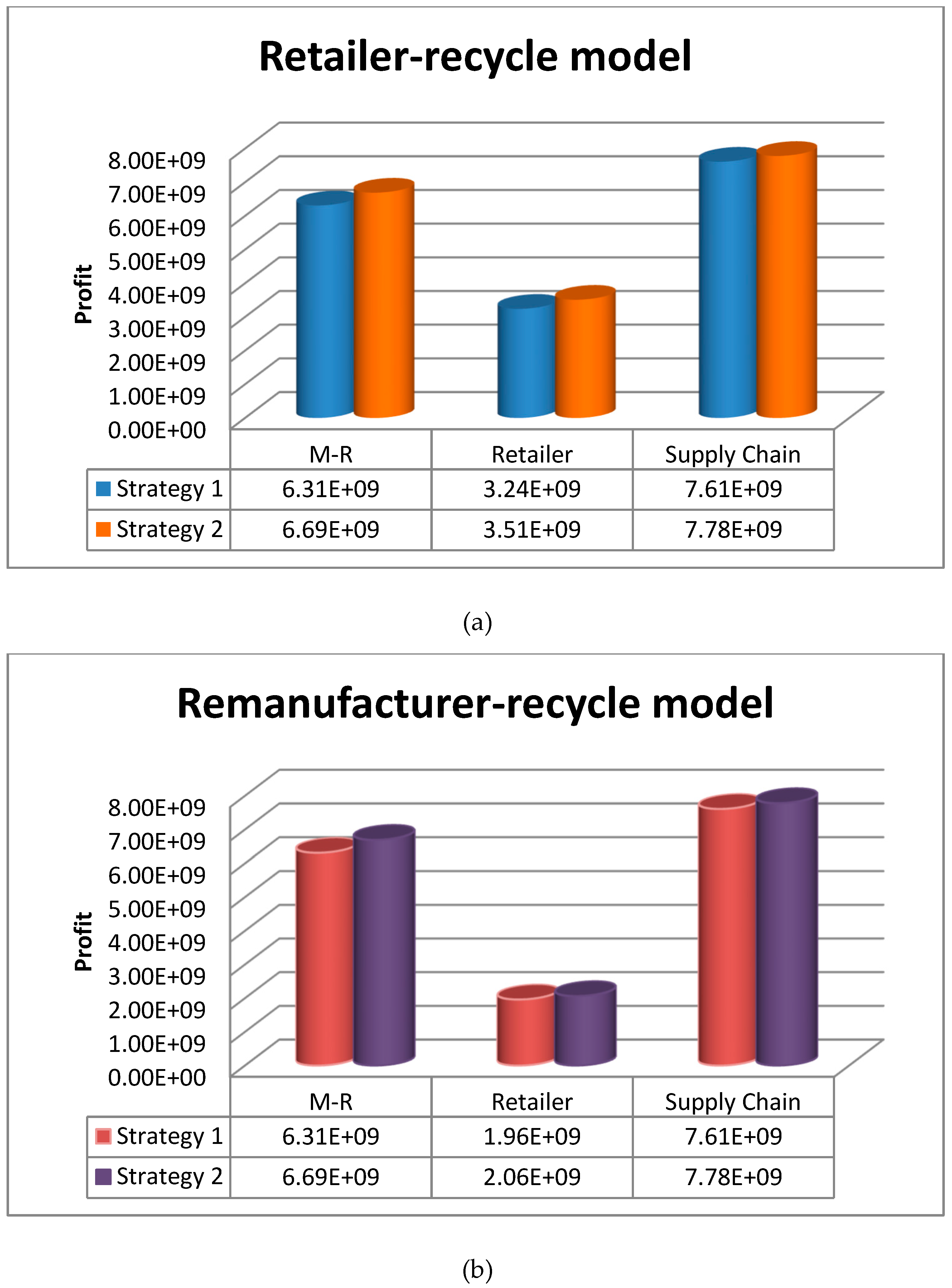
Table 7, respectively. In both remanufacturer-recycle and retailer-recycle models, strategy 2 has a premium on total profit in the three scenarios. The comparisons are shown in
Figure 2. Under acquisition strategy 1, the manufacturer-remanufacturer model and the joint supply chain model have the same recycling target for end-of-use products of each generation. The models suggest collecting the maximum amount of used products from customers, and selling Type 1 and Type 2 products at the equally high prices. However, for the interest of retailer, it is optimal to set up the highest price for Type 1 products and a lower price for Type 2 products, while restricting the recycling of used products. The retailer only wants to collect a few used products belonging to earlier generation models.
Under acquisition strategy 2, the manufacturer and remanufacturer are willing to set the highest price for Type 2 products, a lower price for Type 1 product, and the most economical buyback price for unsold Type 1 products. However, the retailer has a contrasting interest, and prefers to sell Type 1 products at a higher price and Type 2 products at a lower price. The manufacturer-remanufacturer model suggests acquiring the maximum amount of the earliest generation and a median amount of the second earliest generation models, assuming that the new item is still available with the retailer. They are also interested in buying back a considerable amount of unsold new products to fulfil the rest of the demand for Type 2 products. The retailer prefers to collect Generation 4 and return fewer unsold new products. All of them restrict collection to Generation 5 models (the end-of-use products belonging to the latest generation). The joint supply chain model neutralizes the two models.
Table 7 shows the retailer-recycle models under two acquisition strategies. In acquisition strategy 1, all the models suggest an equally high price for Type 1 and Type 2 products. The manufacturer prefers the lowest recycle price of all the generations, while the retailer prefers higher recycle prices for Generation 4 and Generation 5, but lower prices for Generation 4s. The optimal policy for the manufacturer is to collect all used products belonging to different generations, while the retailer tries to minimize the amount of Generation 4s (the same generation model as the Type 1 product). The joint model mitigates the conflict between manufacturer and retailer on buyback pricing decisions, but harmonizes acquisition quantity policy with the manufacturer-remanufacturer model.
Under acquisition strategy 2, the manufacturer-remanufacturer model suggests selling Type 2 products and buying back end-of-use products belonging to the latest generation at the highest rate. For the acquisition quantity, they hope that the retailer will avoid collecting used products belonging to the latest generation. They want more unsold Type 1 products to be returned. The retailer’s model suggests the lowest buying back price for used products belonging to Generation 4s (the same technology level as the Type 1 product), and trying to avoid collecting Generation 4s products, while collecting the latest generation model instead. In addition, the retailer hopes for a lower number of unsold new products to be returned. The joint model mitigates the differences.
By comparing and analyzing the results in the two acquisition strategies above, the conflicting interest of manufacturer and the retailer causes different price decisions and acquisition preferences. The manufacturer tends to gain profit from selling Type 2 products and buying back Type 1 products for upgrading. The retailer prefers to promote Type 1 products. Therefore, the retailer model suggests less return for Type 1 products and less interest in collecting used products belonging to the same generation as Type 1 products.
Figure 3 displays a horizontal comparison. The results of remanufacturer-recycle model and retailer-recycle model are exhibited. The retailer gains significantly more benefit from recycling end-of-use products, while the total profits of the manufacturer-remanufacturer system and the joint supply chain system are indifferent to remanufacturer recycling and retailer recycling. For achieving a win-win, the retailer is the better choice for collecting end-of-use products. This conclusion is also searched by Savaskan and Van Wassenhove [
31].
6.1. Factor Analysis
The characteristics of the two types of products are defined as quality, generation gap, and price. Their market share is based on two factors: customer expectation of the three characteristics, and the product’s performance on the three characteristics. However, customer expectation changes, and the product performance varies over time. Analysis of the two factors reveals insights as to why the optimal solutions in three scenarios differ from each other. The analysis is under the conditions of Strategy 2, in which the retailer takes the responsibility of recycling.
6.1.1. Customers’ Expectation Analysis
The dataset for customer expectation analysis is shown in
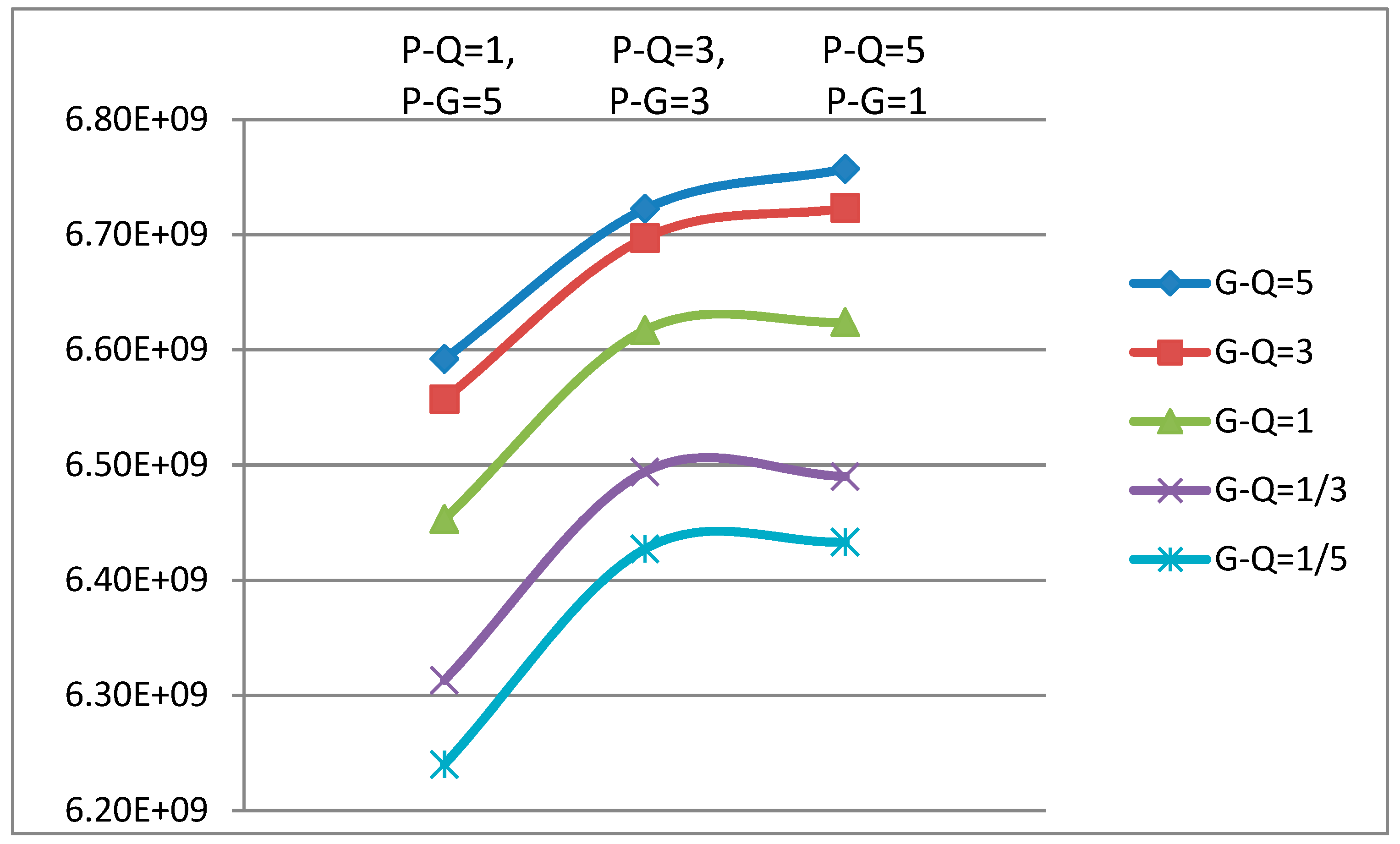
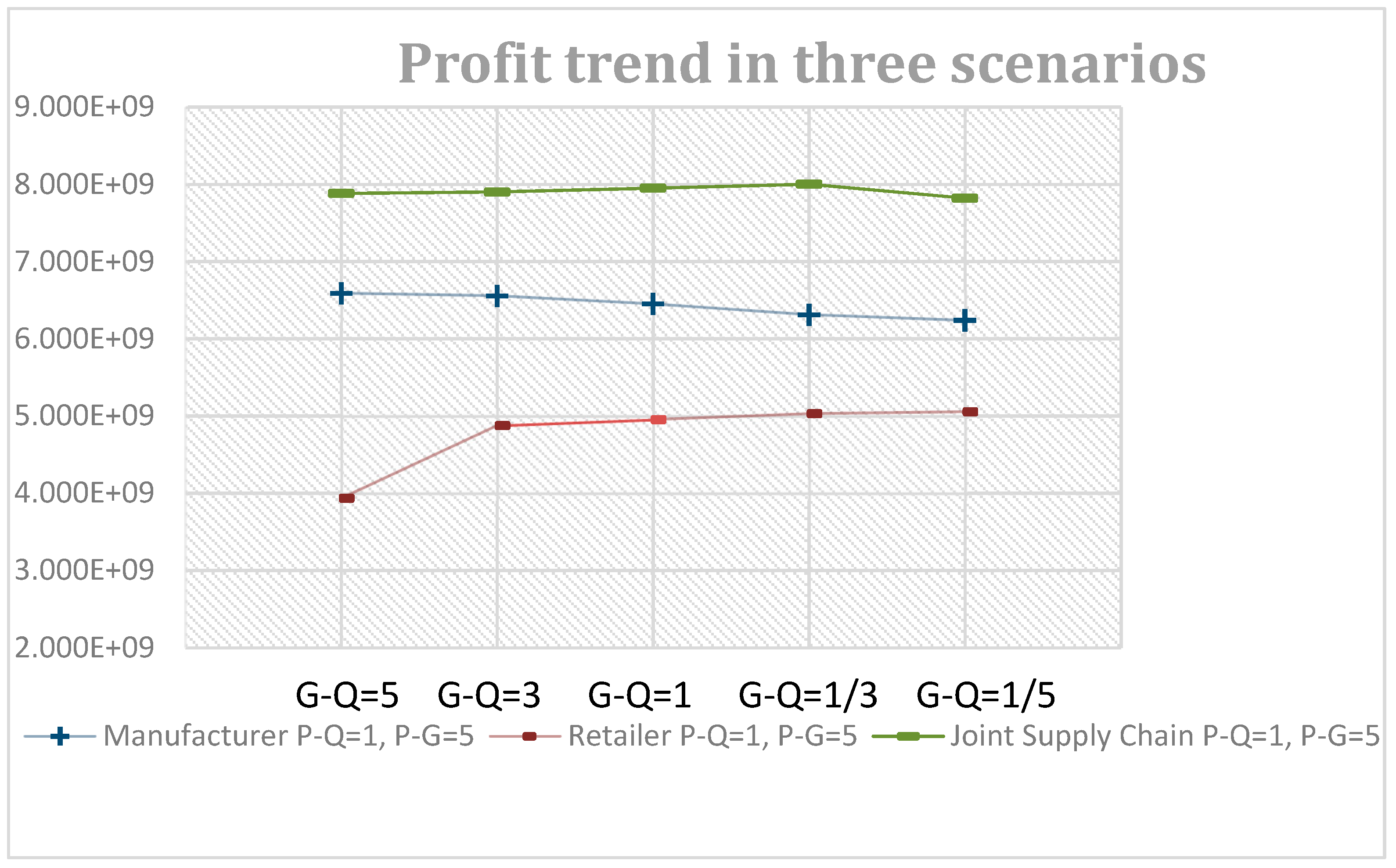
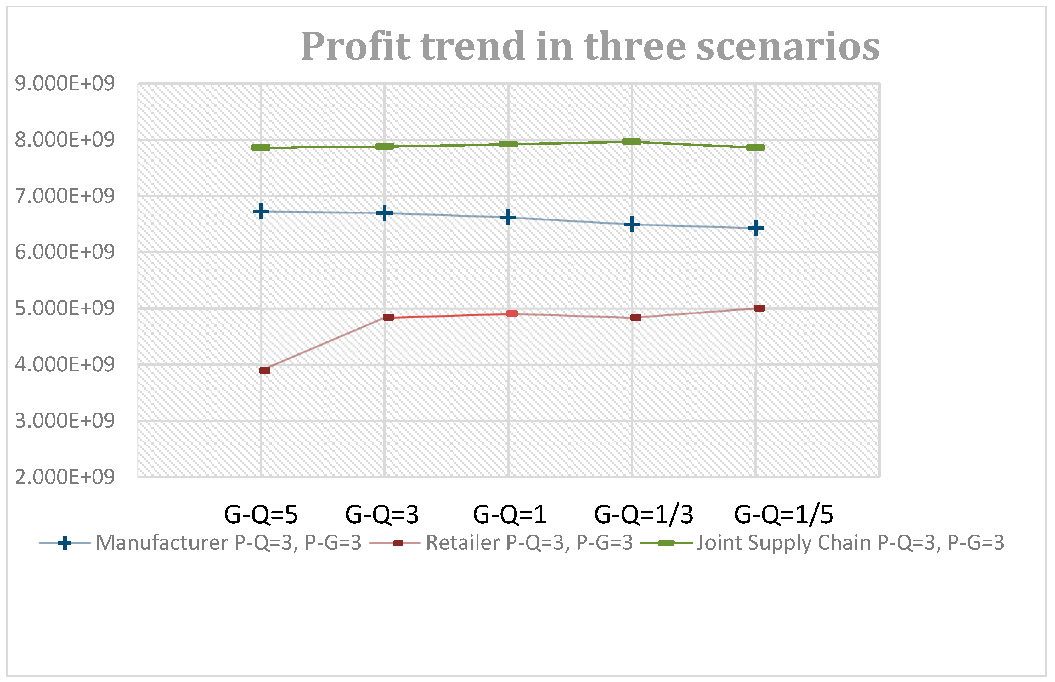
Table 8. “Q” represents “Quality”, “P” represents “Price”, and “G” represents “Generation gap”. The data for products’ performance is the same as the original design based on the assumptions of this paper. The first column shows pair-comparison weight between generation gap and product quality. For example, “G-Q=5” means the perceived value of generation gap is five times important than that of product quality, while “G-Q=1/5” means the perceived weight of generation gap is 1/5 of that of product quality. The second column shows price sensitivity of product quality and generation gap. “P-Q=1, P-G=5” represents the condition that price is more sensitive to generation gap than to quality. “P-Q=3, P-G=3” means equal sensitivity. “P-Q=5, P-G=1” means price is more sensitive to quality than to generation gap. We found that the retailer-recycle model under Strategy 2 has the premium benefit in all three scenarios. In this section, we analyze how customers’ expectations of the three product characteristics influences the profit, price decision and acquisition quantity decision in this policy.
Figure 4,
Figure 5 and
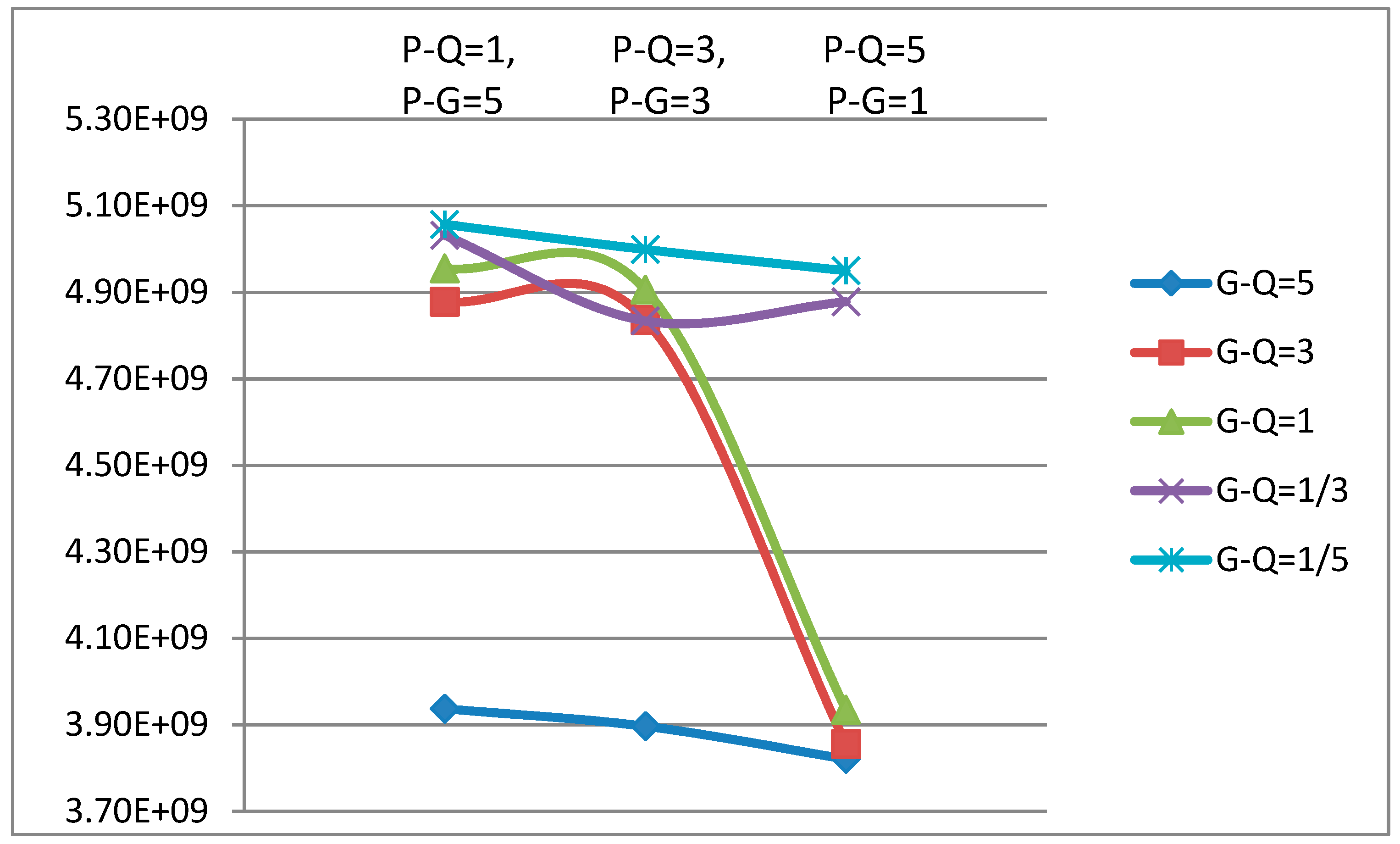
Figure 6 show the profit trends and horizontal comparisons among different conditions in each scenario. In general, manufacturer-remanufacturer profit increases moderately, while the retailer profit and the joint supply chain profit decrease slightly if the price becomes more sensitive to quality and less sensitive to generation gap. However, there is a dramatic profit drop in the retailer’s model when generation is equal to or more important than quality and price is more sensitive to generation gap than quality. The reason for this is that the retailer’s revenue comes from Type 1 products. Type 1 products belong to the earlier generation, which has an advantage in quality but a disadvantage in generation gap. The price of Type 1 products will decrease accordingly.
Figure 7,
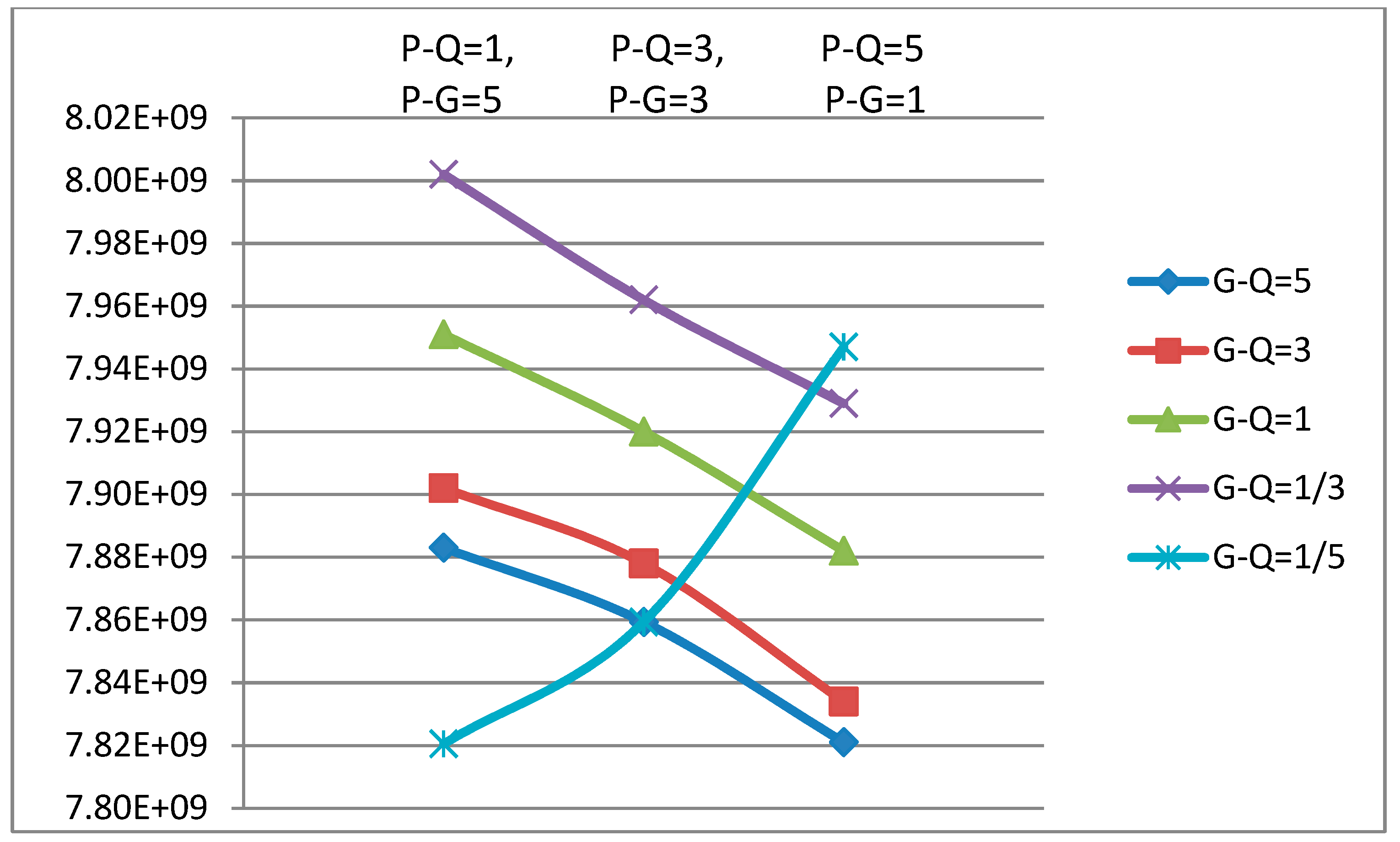
Figure 8 and
Figure 9 show vertical comparisons among three scenarios with different price sensitivities to quality and generation gap. At the same level of price-quality and price-generation gap sensitivity, the manufacturer-remanufacturer profit and the joint supply chain profit increase in general, while the retailer profit decreases if generation gap becomes less important to quality. Another interesting finding in the manufacturer and joint supply chain models is related to the optimal return quantity of overstock new products. The number of returned unsold Type 1 products decreases if the generation gap becomes less critical than quality from customer’s perspective. It is sensible to sell more Type 1 products rather than returning them to upgrade in this condition, because returning to upgrade will decrease the customer’s perceived value of quality.
6.1.2. Product Performance Analysis
Technological innovation does not always take place at the same pace. If the recently introduced new product does not take a large step forward in technological development, the generation gap between Type 1 and Type 2 products will be narrow. We analyzed how the generation gap influences the results. In this analysis, the initial customer expectation dataset is the same, while the generation gap performance is changed to 0.4, 0.6, and 0.8, respectively. The weights of the generation gap performance for Type 1 and Type 2 products are shown in
Table 9. The results are shown in
Table 10.
The manufacturer’s profit will decrease if the new generation model does not take a big step forward in terms of technological innovation, while the retailer profit and the supply chain profit will still increase. Other interesting findings are related to buyback price for end-of-use product belonging to the latest generation, and how many unsold new products should be returned. With the decrease in technological difference, the buyback price for used latest model products is increased in the manufacturer model; the quantity of returned new products is decreased in all three models. This indicates that they are willing to sell new outdated products, as the perceived quality is higher than that of remanufactured ones, while the technology gap is not large enough. To the market of customers who are technology savvy, manufacturers hope to recycle more used latest models in order to satisfy this customer group.
7. Conclusions and Future Study
This paper summarized the market situation and customer purchase behavior towards consumer high-technology products, explaining that the lifespan of these products is not dependent on the time to end-of-life, but the time to end-of-use, as decided by customers. New items also depreciated because of technological obsolesce. Therefore, the idea of returning an optimal number of unsold new products belonging to an earlier generation for upgrading was proposed. We reviewed papers regarding price decisions and launch strategies for short-lifecycle products, key challenges including demand-supply balance and channel design in reverse supply chain, and remanufacturing issues, especially for high-technology products. Although some studies were about pricing decisions for new products across generations, they did not propose remanufactured products as part of the model. Some studies discussed the price decision for new and remanufactured products, but did not consider the condition of multiple generations in the market simultaneously for rapidly developed high-technology products. A few articles investigate the upgrading of new and remanufactured products, but are focused on technological design. The market for new and remanufactured products is not only about price, but the combination of supply chain channel, demand and planning. Some papers have considered the integration of pricing and planning, a few of them have thought to combine the price decision of different acquisition strategies. This paper combined the consideration of generation difference and remanufacturing, found the optimal price for upgraded remanufactured products and out-of-time new products, and collected the quantity for different generation models. The study discussed two acquisition policies: recycle optimal quantity end-of-use products only, and collect both optimal numbers of used products and unsold new products belonging to the earlier generation. It examined the pros and cons of a remanufacturer recycling plan and a retailer recycling plan. The optimal quantity of each generation acquired from customers and the amount of unsold outdated products from the retailer were obtained for different recycle models in all scenarios. Additionally, the analytic hierarchy process (AHP) demand function and the normal distributed returned quantity function were integrated into the model. The AHP method is a combination of customers’ criteria for different product characteristics and the estimated value of the product’s performance. The change of the two factors provided insights for addressing the market share of different types of products. In addition to the new research problem proposed, the AHP method and the analysis of customers’ criteria for different product characteristics were also innovative in the context of research on price decision and acquisition strategy selection for remanufactured high-technology products.
The results indicated a premium for acquiring end-of-use products for remanufacturing and returning the optimal number of unsold outmoded new products for upgrading. A retailer-collect model brings significantly more benefit to the retailer and does not harm the manufacturer and joint supply chain. This sheds light on the remanufacturing opportunity for unsold new products. The model suggested that retailers are the optimal undertaker for collecting used products. Additionally, conflicting interests caused various results for the decision of optimal price and acquisition. Retailers were willing to promote Type 1 products while manufacturers preferred selling remanufactured products. The customer choice demand function expressed that customers make purchase decisions by perceived weight on technological difference, quality and price, and the product’s performance on technology and quality. The changes in customer criteria and product performance gave rise to changes in profit for the manufacturer, the retailer, and the joint supply. The analysis of these changes exhibited how the optimal solution varies in different states. This information gave advice for determining the price and optimal quantity of acquisition and return for different performances in items and particular survey results on customers. The interesting finding was about the condition that the new generation model did not take a big step forward in terms of technological innovation. A slow development caused a reduction in profit for the manufacturer, but the profit for the retailer and the joint supply chain still increased. Also, the optimal number of returned new products decreased. Therefore, manufacturers are recommended to build up more value in technology for the newly released generation model.
Although the study contributes to proposing a new research problem regarding new and remanufactured products across generations and provides managerial insights with respect to how decision making varies based on different customers’ perceived values placed on the product’s characteristics and performance, the paper also has some opportunities to develop in the future. First, the model proposed is a general model that does not represent any cases in the real world. For the specific items, the design for forward and reverse supply chain, transportation, logistics, and planning should be adjusted accordingly. Second, more factors could be integrated into the model, such as the segments of the low-end and high-end products, the upgrading technique barrier, and technology characteristics. Third, the model can be extended to a multi-period problem with a dynamic maximum demand utility over time. Finally, the lead time and product quality can be considered to be followed by a probabilistic distribution. The probabilistic delivery cost would be added to the model accordingly.


