Intermittent and Adaptive Control Strategies for Chaos Suppression in a Cancer Model

Abstract

The chaotic dynamics observed in mathematical models of cancer can correspond to the unpredictable tumor growth and treatment responses seen in clinical settings. Suppressing this chaos is a significant challenge in theoretical oncology. This paper investigates and compares four distinct control strategies designed to stabilize a chaotic three-dimensional tumor-immune interaction model. The objective is to steer the system from its chaotic attractor to a target unstable periodic orbit, representing a transition to a more regular and predictable dynamic. The strategies, all based on the external force control paradigm, include continuous control, a simple state-dependent intermittent control, an improved intermittent control with a minimum activation duration to suppress chattering, and an adaptive intermittent control with a time-varying feedback gain. The performance of each strategy is quantitatively evaluated based on tracking accuracy and the required control effort.

1. Introduction

Chaos theory describes complex dynamical systems that are highly sensitive to initial conditions, leading to unpredictable and irregular behavior over time. The stabilization of such systems, a process known as chaos control, is achieved by applying small, carefully timed perturbations that guide the system toward a desired state or trajectory. Over the past decades, numerous strategies have been developed to suppress chaotic dynamics in various physical, biological, and engineering contexts. Methodological advancements range from general frameworks like model-free deep reinforcement learning [1] or the partial control method for maintaining trajectories within safe bounds [2] to highly specialized applications.

In engineering and physics, for instance, recent studies have applied these techniques to solve challenges in robotics, such as the control of under-actuated robot manipulators [3], and to stabilize high-dimensional mechanical systems like double rotor models [4]. Applications extend to aerospace for the control of chaotic satellite systems [5] and to materials science for optimizing crystal growth processes [6]. Further applications include manipulating chaos in cavity optomechanical systems for secure communications [7,8] and securing digital media with chaotic watermarking [9]. The principles of chaos control are equally impactful in stabilizing population dynamics in ecological models, such as those for host–parasitoid or prey–predator interactions [10,11,12]. In medicine, recent applications of chaos control range from suppressing spiral-wave chaos in cardiac arrhythmias using low-energy electrical pulses [13,14] to analyzing epidemiological models for diseases like syphilis to better understand stabilization [15]. In economics, chaos control can be used to investigate and manage the stability of econometric systems, providing insights into economic cycles [16].

The principles of chaos control are particularly relevant to oncology. While the term chaos is often used colloquially in oncology to describe the seemingly disordered and complex nature of tumor progression [17], it is crucial to distinguish this from its rigorous mathematical definition. Specifically, the rapid or unbounded growth of cancer cells, a hallmark of the disease, is not a form of deterministic chaos. Mathematically, chaotic dynamics are intrinsically bounded—the system’s evolution is confined to a finite region in phase space known as a strange attractor [18]. Unbounded growth, in contrast, represents a trajectory that diverges to infinity and is typically an artifact of models that do not incorporate realistic biological constraints, such as nutrient and space limitations [19]. In the context of cancer-immune models, true chaos signifies a more complex phenomenon: a sustained, irregular, and unpredictable interaction between the tumor and the host immune system. This mathematically defined chaotic behavior corresponds to the irregular tumor growth patterns and unpredictable responses to therapies that can lead to treatment resistance and disease progression [20]. Recent studies emphasize the significant role that deterministic chaos can play in cancer progression, particularly in cellular networks, gene expression patterns, and tumor-immune system interactions [21,22,23]. Other mathematical frameworks, such as integro-differential systems based on the kinetic theory of active particles, have also been developed to analyze the complex interactions and blow-up phenomena of cancer cells under immune response [24]. This highlights the critical need for mathematical modeling to understand and ultimately control the chaotic behaviors inherent to cancer systems [25].

In response to this challenge, various chaos control strategies have been adapted for cancer models. These approaches aim to stabilize unpredictable tumor dynamics, guiding the system toward a steady or periodic state. Methods range from continuous feedback control, with which interventions like chemotherapy are modeled as persistent inputs [26], to adaptive control, which adjusts inputs in response to system errors, as demonstrated by the controller in [27] that effectively stabilizes tumor and immune cell counts. Another prominent strategy is optimal control, which seeks to identify the most effective intervention based on a predefined set of objectives. This approach has been used to derive necessary controller inputs for achieving asymptotic stability, even in systems with unknown parameters [28], and to manage complex dynamics like cancer self-remission [29]. Optimal control is also applied for designing clinically relevant strategies like combinatorial therapies that maximize immune response while minimizing tumor size and drug toxicity [30]. To solve these complex optimization problems, especially in non-linear fractional-order systems, some studies employ computational methods like particle swarm optimization and genetic algorithms to find the ideal drug dosing [31]. Another analytical approach involves state-space exact linearization, which employs nonlinear feedback based on Lie algebra to transform the original chaotic system into a linear, controllable one [32]. Beyond these, other techniques such as state feedback and hybrid control have been applied to mitigate chaotic behavior, particularly in discretized fractional-order models that describe the tumor-immune interaction in both benign and malignant cases [33].

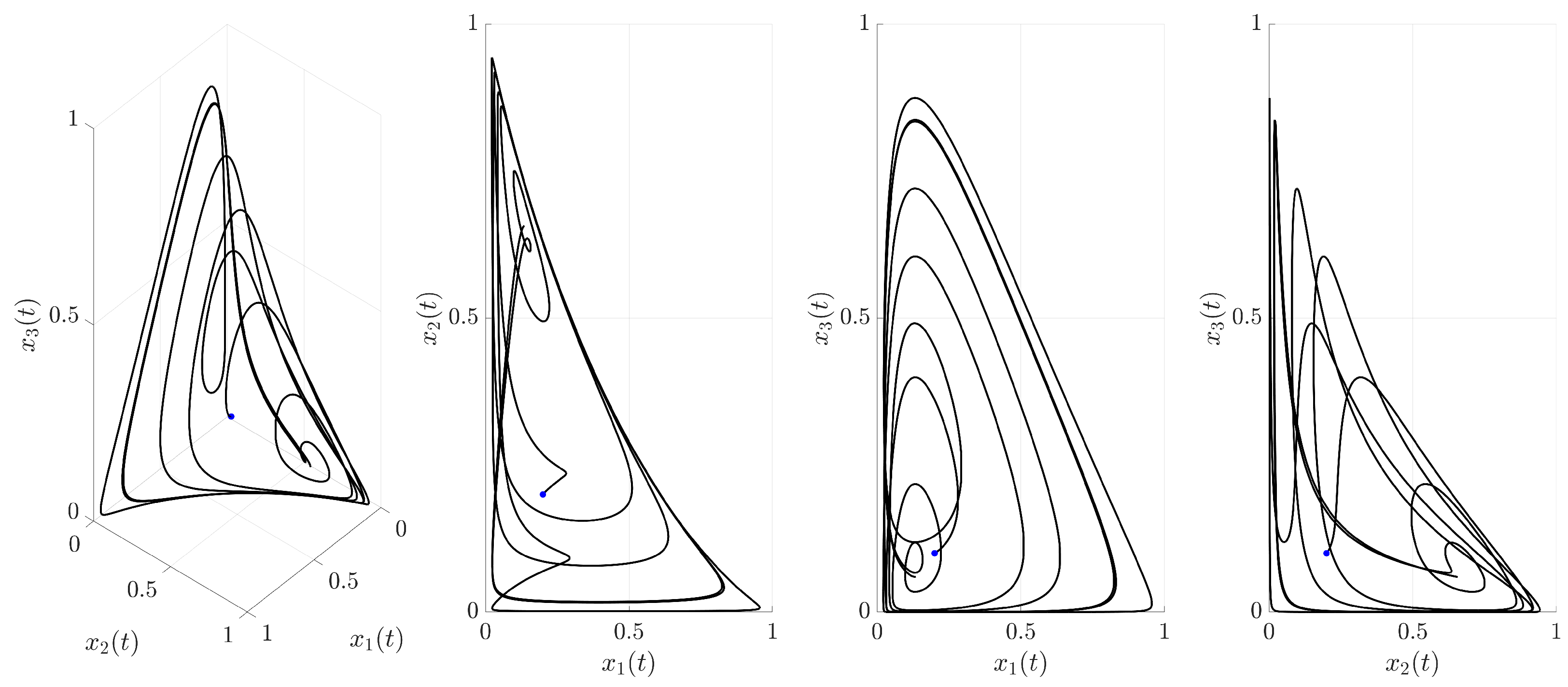
This study investigates the chaotic dynamics of the three-dimensional cancer model presented in [34], which describes the complex interactions between tumor cells, healthy tissue, and the activated immune system. While the original work rigorously established the existence of chaos in this system, the primary aim of this paper is to compare the efficacy of several distinct strategies for controlling these chaotic dynamics. All strategies investigated in this paper share a common theoretical framework: that of exogenous intervention, where an external corrective force is applied to a system that is already in a chaotic state. The objective is the complete suppression of the chaotic dynamics and the stabilization of the involved populations onto a specific, regular, unstable periodic orbit. This approach differs fundamentally from studies that use bifurcation analysis to understand how chaos can be managed or delayed by tuning the system’s endogenous parameters. For instance, a recent study on a prey–predator model demonstrated that predator-induced fear can act as an intrinsic parameter that effectively delays the onset of chaos and stabilizes population dynamics under certain conditions [35]. In contrast, our work addresses the challenge of imposing stability when the system’s biological parameters are already fixed within a chaotic regime, a scenario that is highly relevant to clinical applications where a patient’s underlying system parameters cannot be easily altered. With this framework in mind, the investigation in this study begins with continuous control to establish a baseline for stabilization. Subsequently, intermittent control is explored as a strategy to reduce the therapeutic burden by activating interventions only when the system deviates from a target trajectory. This approach is then refined into an improved intermittent strategy that incorporates a minimum activation duration to suppress undesirable high-frequency switching. Finally, an adaptive intermittent control strategy is introduced, designed to account for inherent uncertainties by allowing control parameters to adjust automatically. A central goal of this paper is to provide a comparative analysis of these methods, evaluating their efficiency, responsiveness, and biological relevance for stabilizing this well-established cancer model. A key motivation for exploring intermittent strategies is the recognition that continuous interventions, while effective in mathematical models, often translate poorly to clinical settings due to issues like drug toxicity, patient burden, and the development of resistance. Therefore, this study places particular emphasis on control methods that reduce the overall therapeutic intervention.

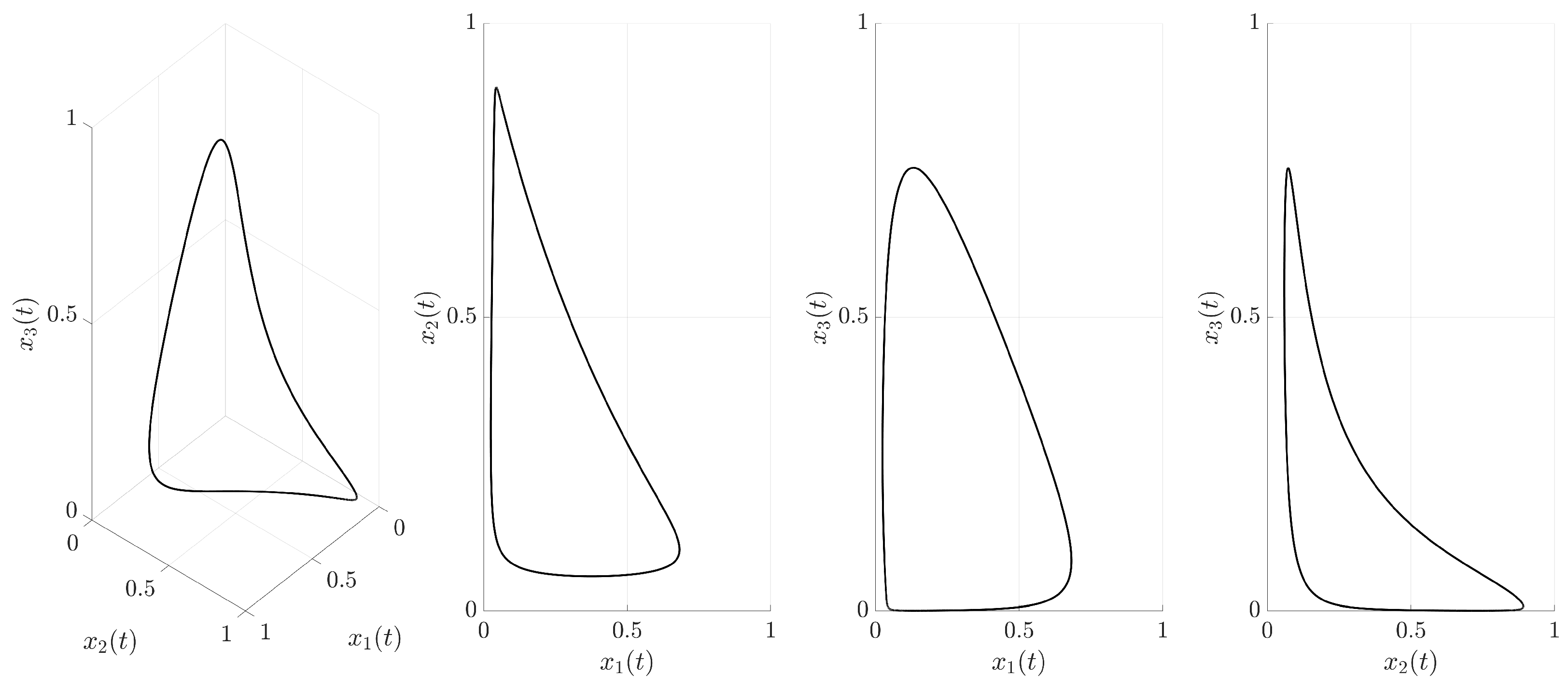
The remainder of this paper is structured as follows. Section 2 addresses the materials and methods: Section 2.1 describes the analyzed mathematical model and its chaotic dynamics, Section 2.2 details the identification of the target unstable periodic orbit, and Section 2.3 establishes the general framework for the applied techniques. Section 3 contains the main results, presenting several chaos suppression strategies. These include continuous external force control (Section 3.1), intermittent control (Section 3.2), an improved intermittent strategy with a minimum activation duration (Section 3.3), and adaptive intermittent control (Section 3.4). A comparative evaluation of these methods is provided in Section 3.5. Concluding remarks are given in the final Section 4.

2. Materials and Methods

2.1. The Cancer Model and Its Chaotic Dynamics

The mathematical framework for this study is the three-dimensional cancer model developed by Itik and Banks in [34], which describes the interactions among tumor cells, healthy host cells, and effector immune cells. After nondimensionalization, the model’s dynamics are governed by the following system of ordinary differential equations (ODEs):

$$\begin{array}{cc}\hfill \frac{{\mathrm{d}x}_1}{\mathrm{d}t}& =x_1(1-x_1)-a_{12}{x}_1{x}_2-a_{13}{x}_1{x}_3;\hfill \\ \hfill \frac{{\mathrm{d}x}_2}{\mathrm{d}t}& =r_2{x}_2(1-x_2)-a_{21}{x}_1{x}_2;\hfill \\ \hfill \frac{{\mathrm{d}x}_3}{\mathrm{d}t}& ={\displaystyle \frac{r_3{x}_1{x}_3}{x_1+k_3}}-a_{31}{x}_1{x}_3-d_3{x}_3.\hfill \end{array}$$

(1)

In this system, $x_1\left(t\right)$, $x_2\left(t\right)$, and $x_3\left(t\right)$ represent the normalized population densities of tumor cells, healthy host cells, and effector immune cells, respectively. The model incorporates logistic growth for both tumor cells, $x_1(1-x_1)$, and healthy host cells, $r_2{x}_2(1-x_2)$, where the parameter $r_2$ is the ratio of the host cell growth rate to that of the tumor cells. The parameters $a_{12}$ and $a_{13}$ represent the scaled rates at which tumor cells are lost due to competition with healthy cells and predation by immune cells, respectively. Conversely, $a_{21}$ is the rate at which healthy cells are lost due to interactions with tumor cells. The immune response is modeled by the term ${\displaystyle \frac{r_3{x}_1{x}_3}{x_1+k_3}}$, which describes the stimulation of effector cells by the tumor, exhibiting saturation kinetics with a maximum stimulation rate related to $r_3$ and a scaled saturation constant, $k_3$. The parameter $a_{31}$ accounts for the inactivation of immune cells through interaction with tumor cells, and $d_3$ represents their natural death rate. As noted in [34], the model assumes that effector cells require activation by tumor antigens, and thus omits a constant influx term for these cells.

It was demonstrated in [34] that system (1) exhibits chaotic dynamics for the following parameter set, which is adopted for this study: $a_{12}=1$, $a_{13}=2.5$, $a_{21}=1.5$, $r_2=0.6$, $a_{31}=0.2$, $d_3=0.5$, $r_3=4.5$, and $k_3=1$. With these parameters, the system displays a chaotic attractor, as depicted in Figure 1. While the original work focused on characterizing this chaotic behavior, the present study aims to control it. The primary objective is to suppress the chaotic dynamics by stabilizing an unstable periodic orbit embedded within the strange attractor, which could correspond to a more predictable and therapeutically desirable state.

2.2. Identification of the Target Unstable Periodic Orbit

Unstable periodic orbits (UPOs) are fundamental structures embedded within chaotic attractors, and their identification is a prerequisite for many chaos control techniques. Standard numerical methods, such as those based on finding recurrences on a Poincaré section, can locate these orbits. Once an approximate UPO is found, iterative refinement algorithms, like the Newton–Raphson method, can be applied to the periodicity constraint $\mathbf{x}\left(T\right)=\mathbf{x}\left(0\right)$ to precisely determine the orbit and its period, T.

Using such numerical techniques, a specific UPO within the chaotic attractor of system (1) was identified to serve as the target for the control strategies investigated in this paper. This target UPO, denoted as ${\mathbf{x}}^{\left(UPO\right)}\left(t\right)=\left(x_1^{\left(UPO\right)}\left(t\right),x_2^{\left(UPO\right)}\left(t\right),x_3^{\left(UPO\right)}\left(t\right)\right)$, is illustrated in Figure 2. This trajectory represents the dynamic behavior that the control algorithms presented in the subsequent sections will attempt to stabilize.

The specific UPO shown in Figure 2 was selected as a representative target to facilitate a clear and rigorous comparison of the different control strategies. The primary focus of this study is on the mechanics, efficiency, and comparative performance of the control frameworks themselves, rather than on the identification of an optimal therapeutic trajectory. However, it is important to note that, in any potential clinical application, the choice of the target orbit can have significant therapeutic implications. An ideal therapeutic goal would not be to stabilize just any periodic orbit, but to identify and stabilize a UPO characterized by patient-beneficial properties, such as a low average tumor cell population and a high, persistent immune cell population. The systematic search for and classification of such optimal UPOs within a chaotic attractor is a valuable and complex research topic in its own right, but it falls beyond the scope of this methodological paper. Therefore, the chosen UPO serves as a consistent and suitable benchmark against which the different chaos control methods can be evaluated.

2.3. Control Strategy Framework

With the target UPO identified, the core of this study involves applying and comparing several strategies designed to stabilize this orbit and suppress the system’s chaotic dynamics. All implemented control approaches are based on the concept of external force control introduced in [36], where a corrective force, $\mathbf{F}\left(t\right)$, is added to the system dynamics. The goal is to steer the system state, $\mathbf{x}\left(t\right)$, from an arbitrary initial condition within the chaotic attractor towards the desired UPO and maintain it there.

The general form of the controlled system is thus described as follows:

$$\frac{\mathrm{d}\mathbf{x}}{\mathrm{d}t}=\mathbf{f}(\mathbf{x})+\mathbf{F}(t),$$

(2)

where $\mathbf{x}\left(t\right)=\left(x_1\left(t\right),x_2\left(t\right),x_3\left(t\right)\right)$ is the state vector, $\mathbf{f}\left(\mathbf{x}\right)$ represents the original uncontrolled system dynamics, and $\mathbf{F}\left(t\right)$ is the external control force vector, applied component-wise to the state vector.

The specific form of $\mathbf{F}\left(t\right)$ varies for each strategy. The investigation presented in the next section begins with a standard continuous control to establish a performance baseline, followed by an analysis of intermittent control and its refined, chatter-suppressed variant, and concludes with an adaptive intermittent strategy. Each method’s performance is evaluated to compare the trade-offs between stabilization accuracy and control effort.

3. Results

3.1. Continuous External Force Control

The first strategy investigated is continuous external force control. This method applies a corrective force that is always active (for $t>0$) and is proportional to the error between the current system state, $\mathbf{x}\left(t\right)$, and the corresponding state of the target UPO, ${\mathbf{x}}^{\left(UPO\right)}\left(t\right)$. This control force is defined as follows:

$$\mathbf{F}\left(t\right)=K\left({\mathbf{x}}^{\left(UPO\right)}\left(t\right)-\mathbf{x}\left(t\right)\right),$$

(3)

where $K>0$ is an adjustable control parameter determining the strength of the corrective action. Incorporating this control force into the system dynamics (1) yields the following set of controlled equations:

$${\dot{x}}_1=x_1(1-x_1)-a_{12}{x}_1{x}_2-a_{13}{x}_1{x}_3+K\left(x_1^{\left(UPO\right)}-x_1\right);$$

(4)

$${\dot{x}}_2=r_2{x}_2(1-x_2)-a_{21}{x}_1{x}_2+K\left(x_2^{\left(UPO\right)}-x_2\right);$$

(5)

$${\dot{x}}_3={\displaystyle \frac{r_3{x}_1{x}_3}{x_1+k_3}}-a_{31}{x}_1{x}_3-d_3{x}_3+K\left(x_3^{\left(UPO\right)}-x_3\right).$$

(6)

This control is applied continuously for $t\ge 0$. The effectiveness of this continuous control strategy, using $K=5$, is visualized in Figure 3, Figure 4 and Figure 5. Note that the value of K was selected based on preliminary numerical simulations as a value sufficient to achieve robust stabilization, thereby providing a consistent parameter to fairly compare the performances of the different control strategies.

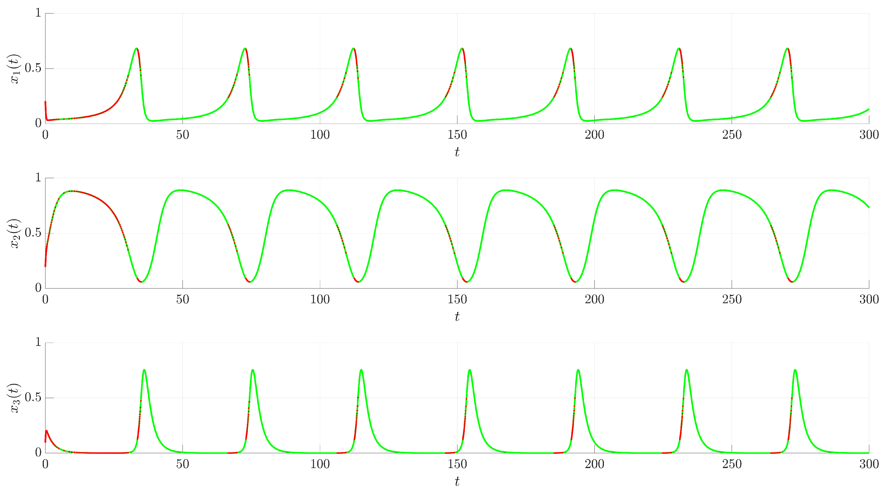
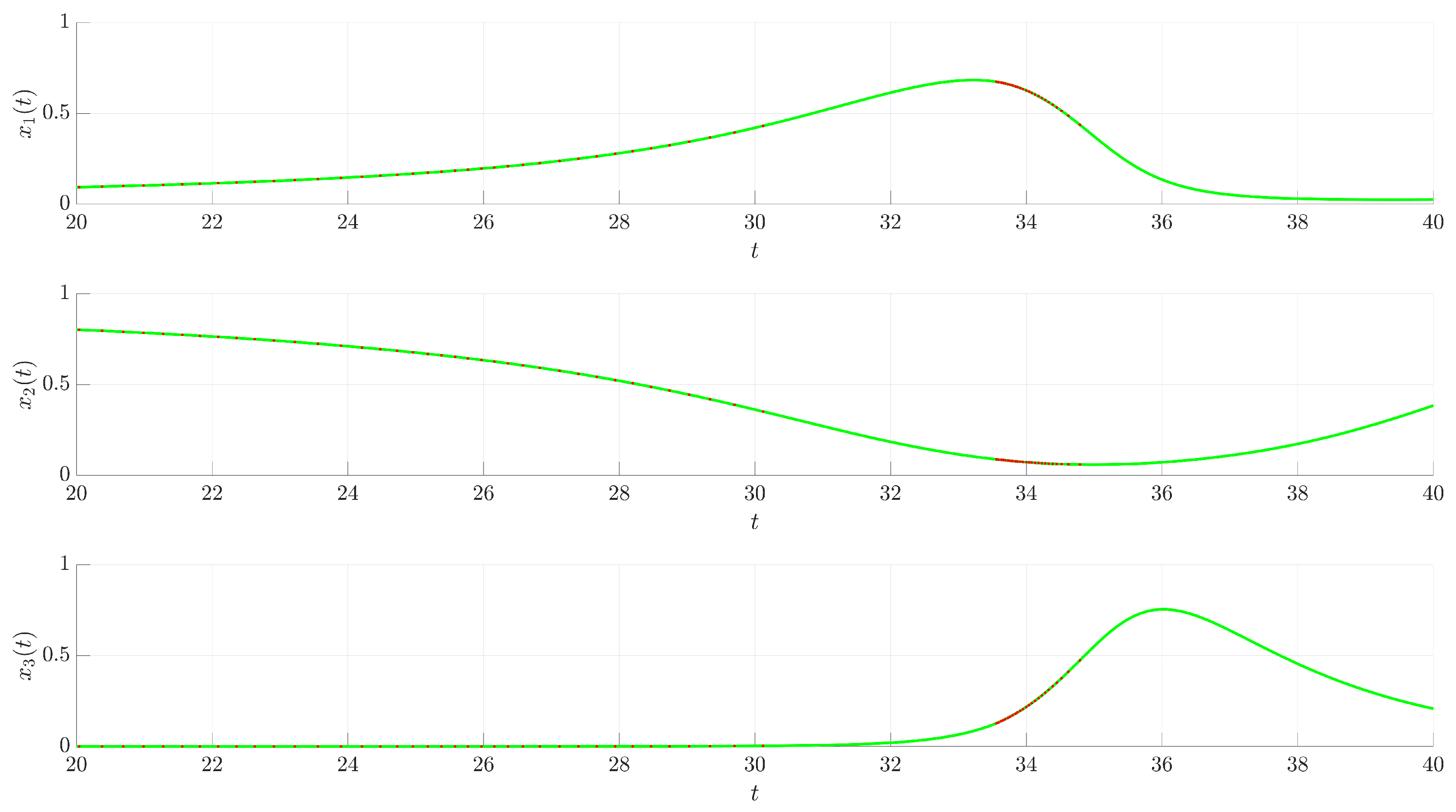
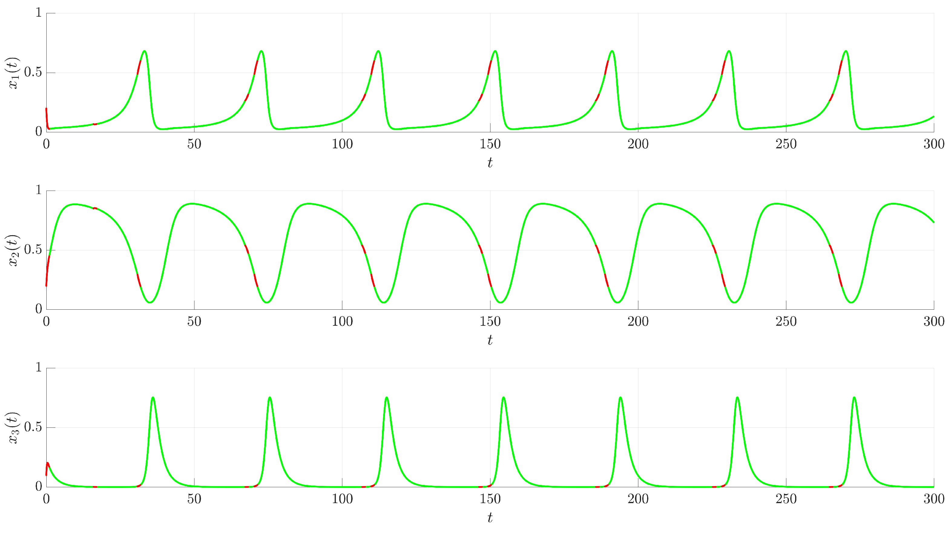
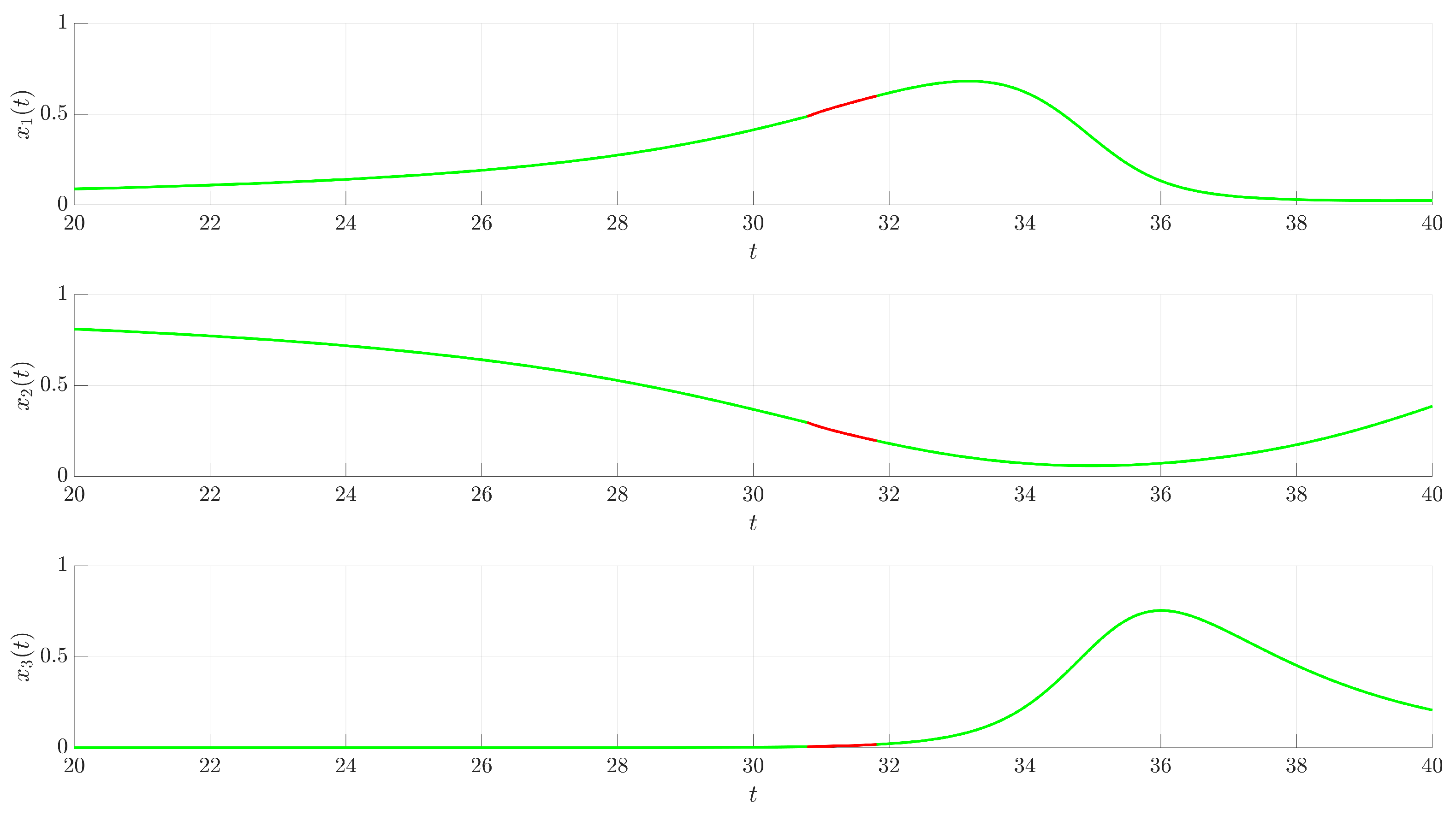
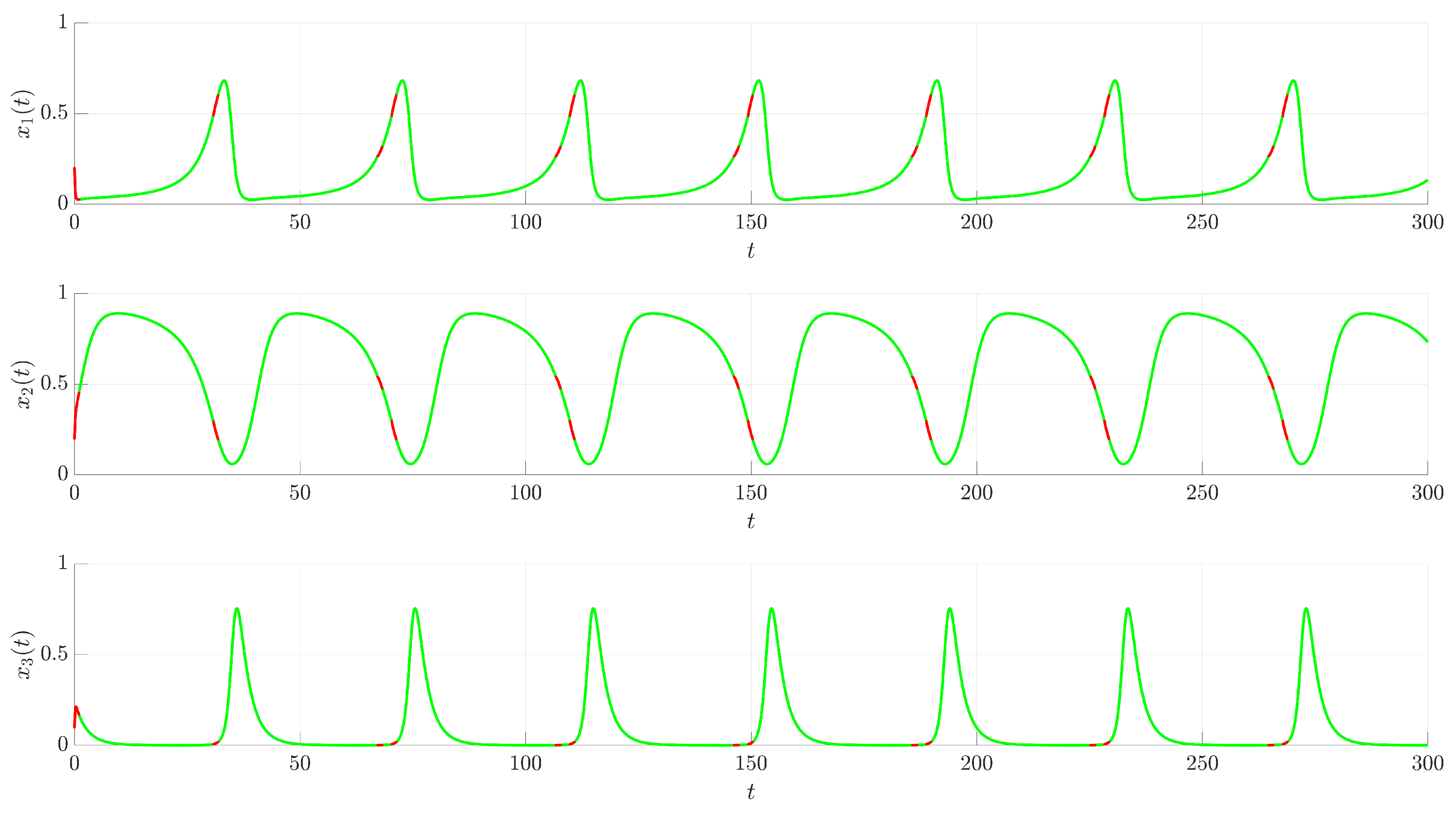
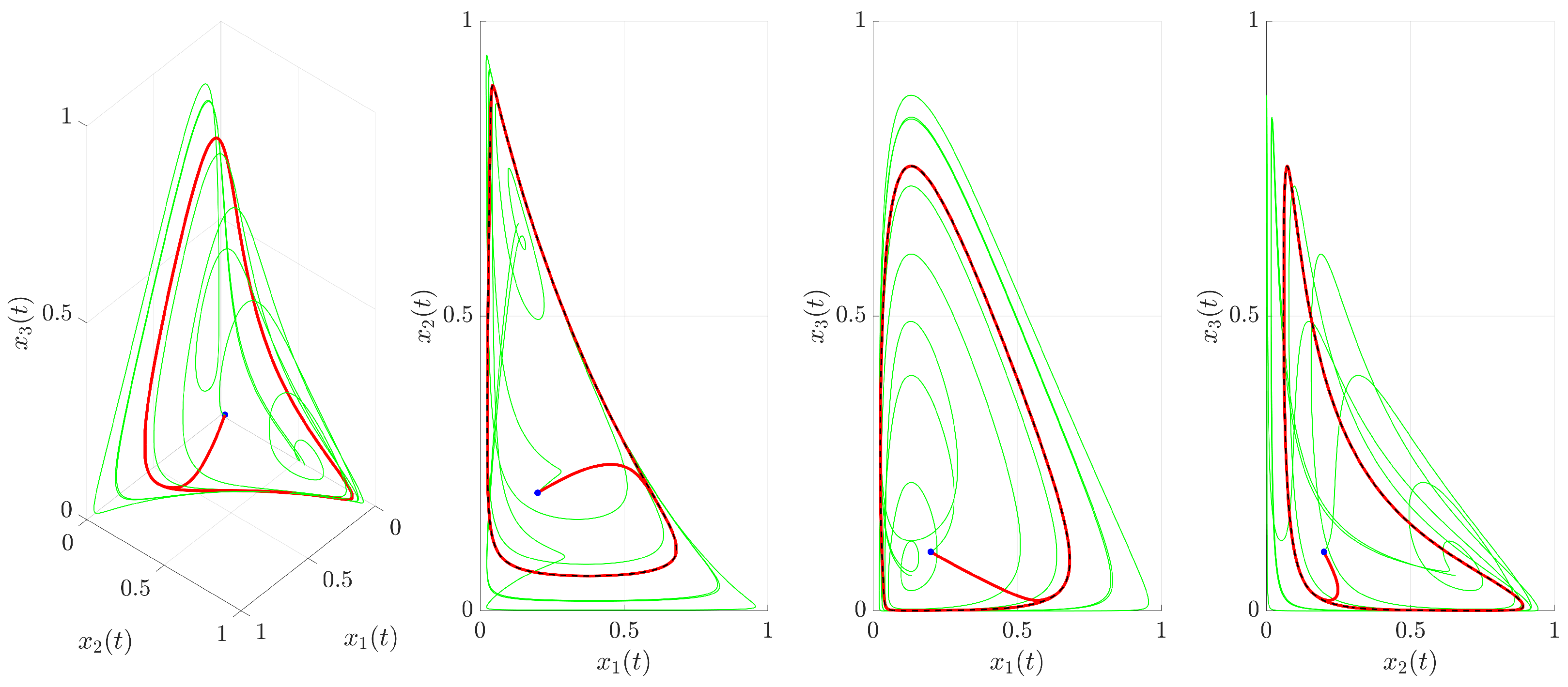
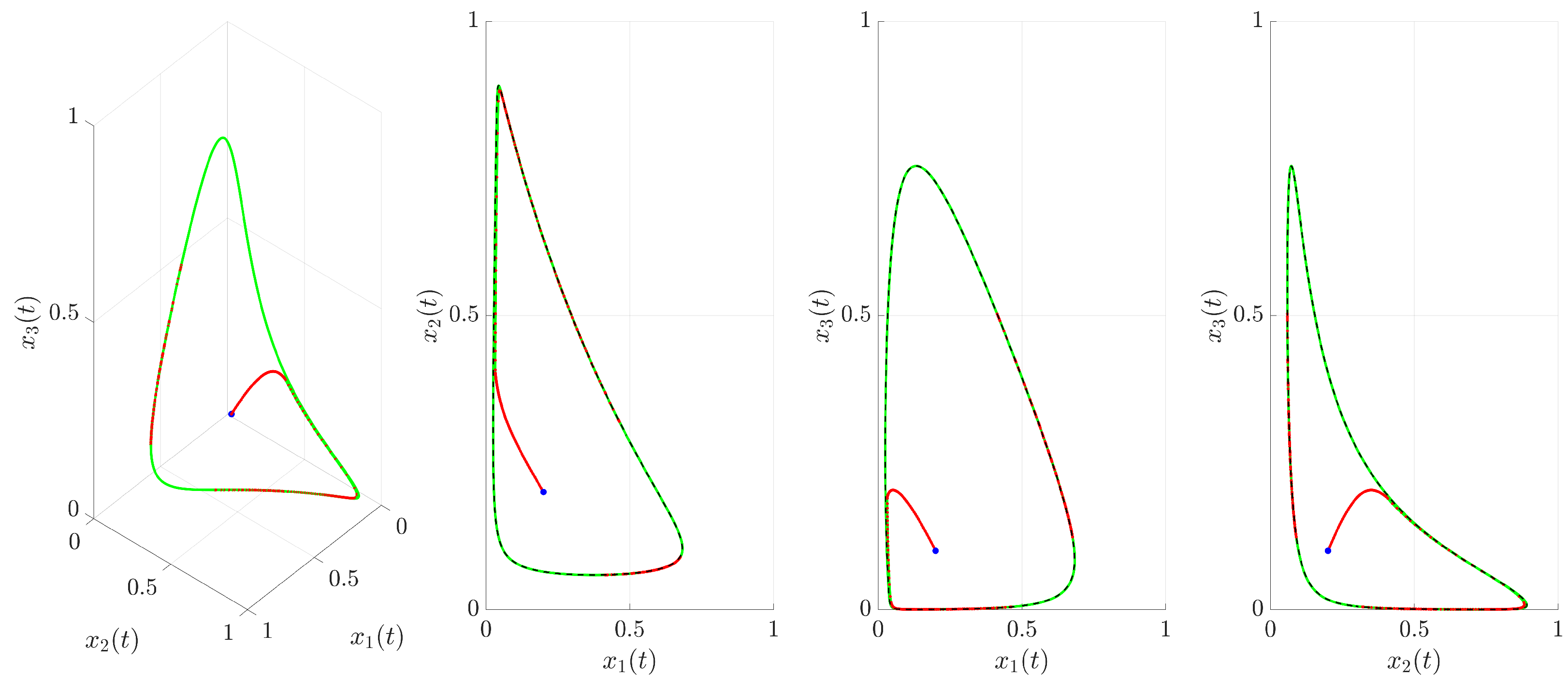
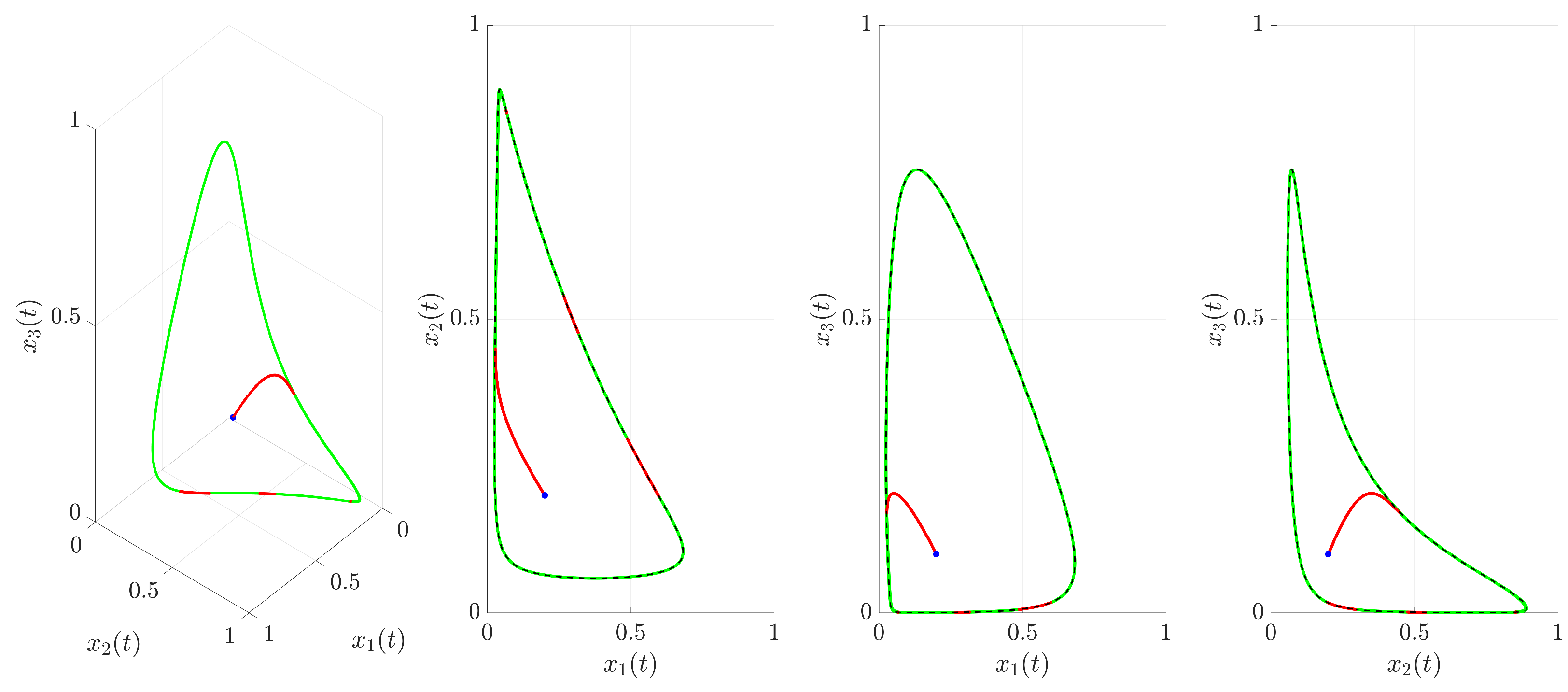
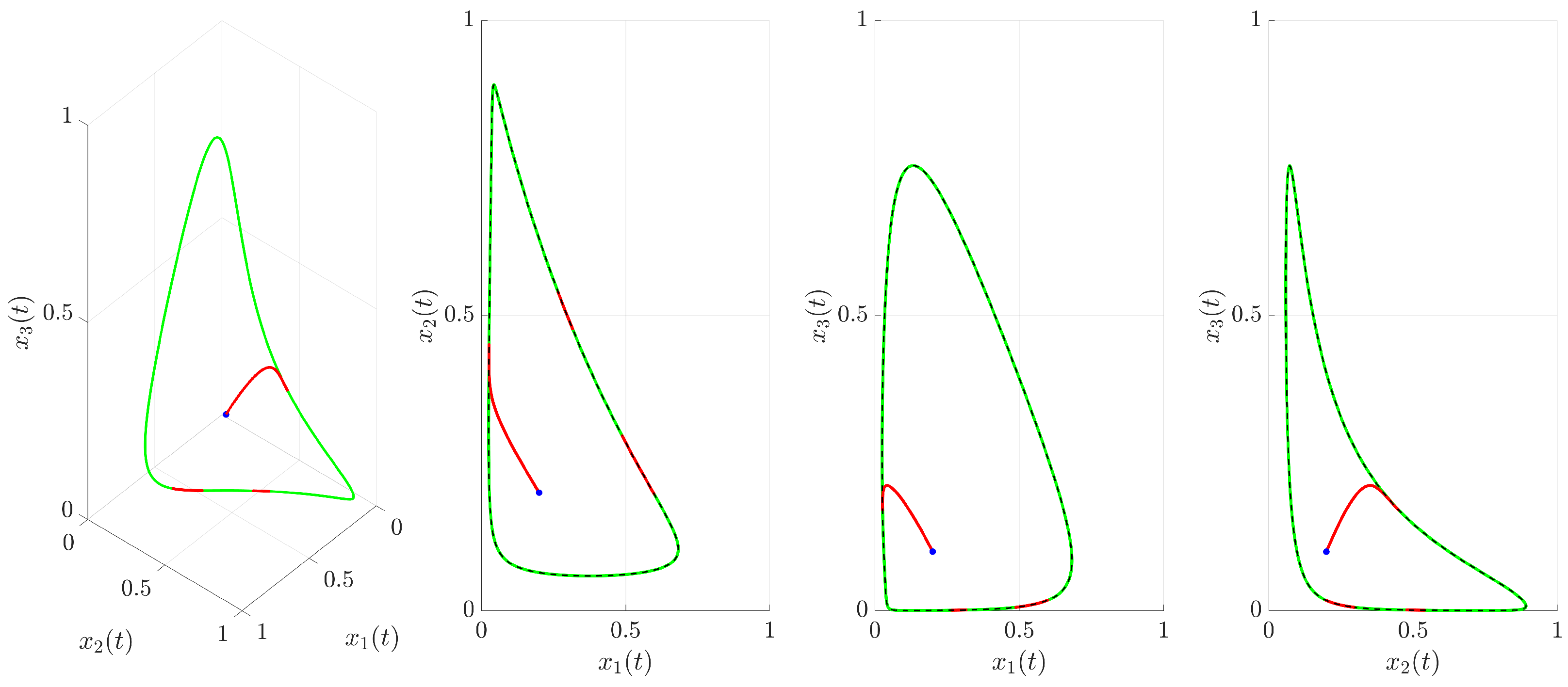
Figure 3 illustrates the time evolution of the state variables $x_1\left(t\right)$, $x_2\left(t\right)$, and $x_3\left(t\right)$. For comparison, the uncontrolled chaotic trajectory originating from the same initial condition is shown in green. When the continuous control is activated at $t=0$ (red trajectory), the state variables rapidly converge to a regular, periodic pattern corresponding to the target UPO. This demonstrates the control’s ability to suppress the inherent chaotic dynamics and enforce the desired periodic behavior. 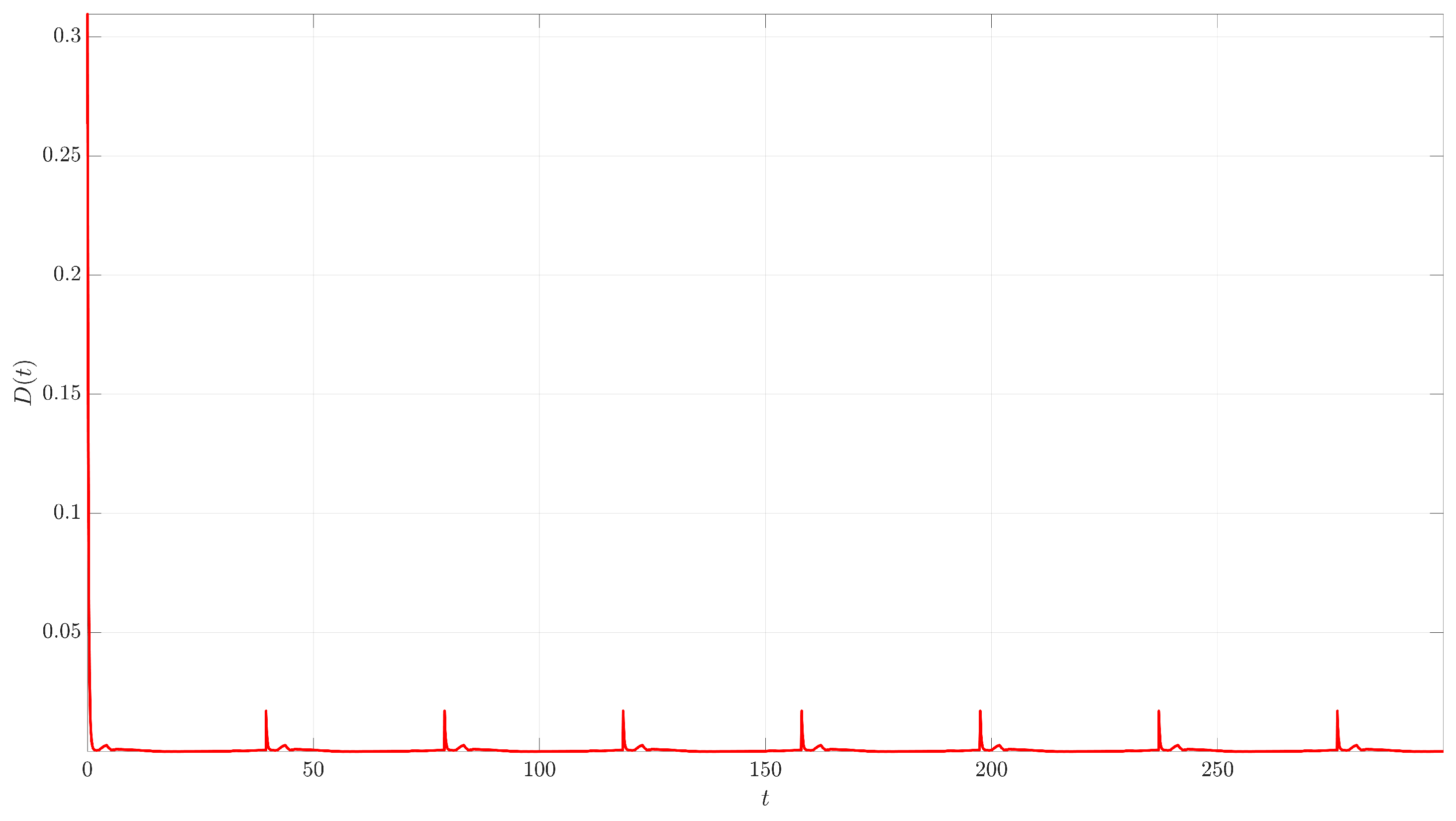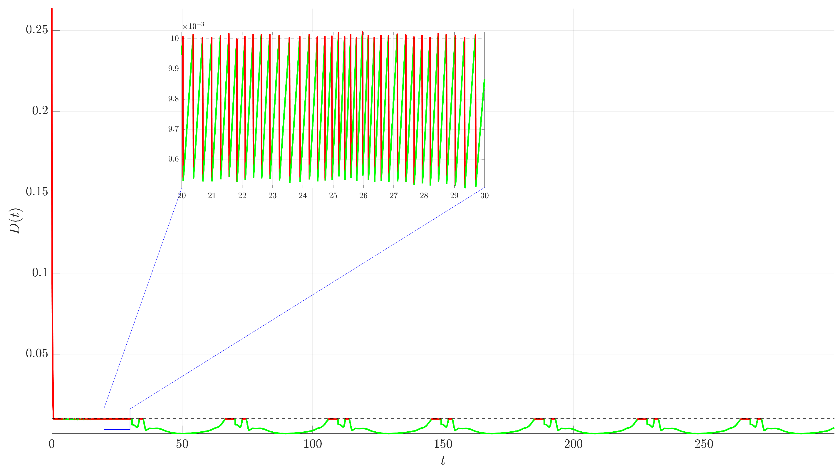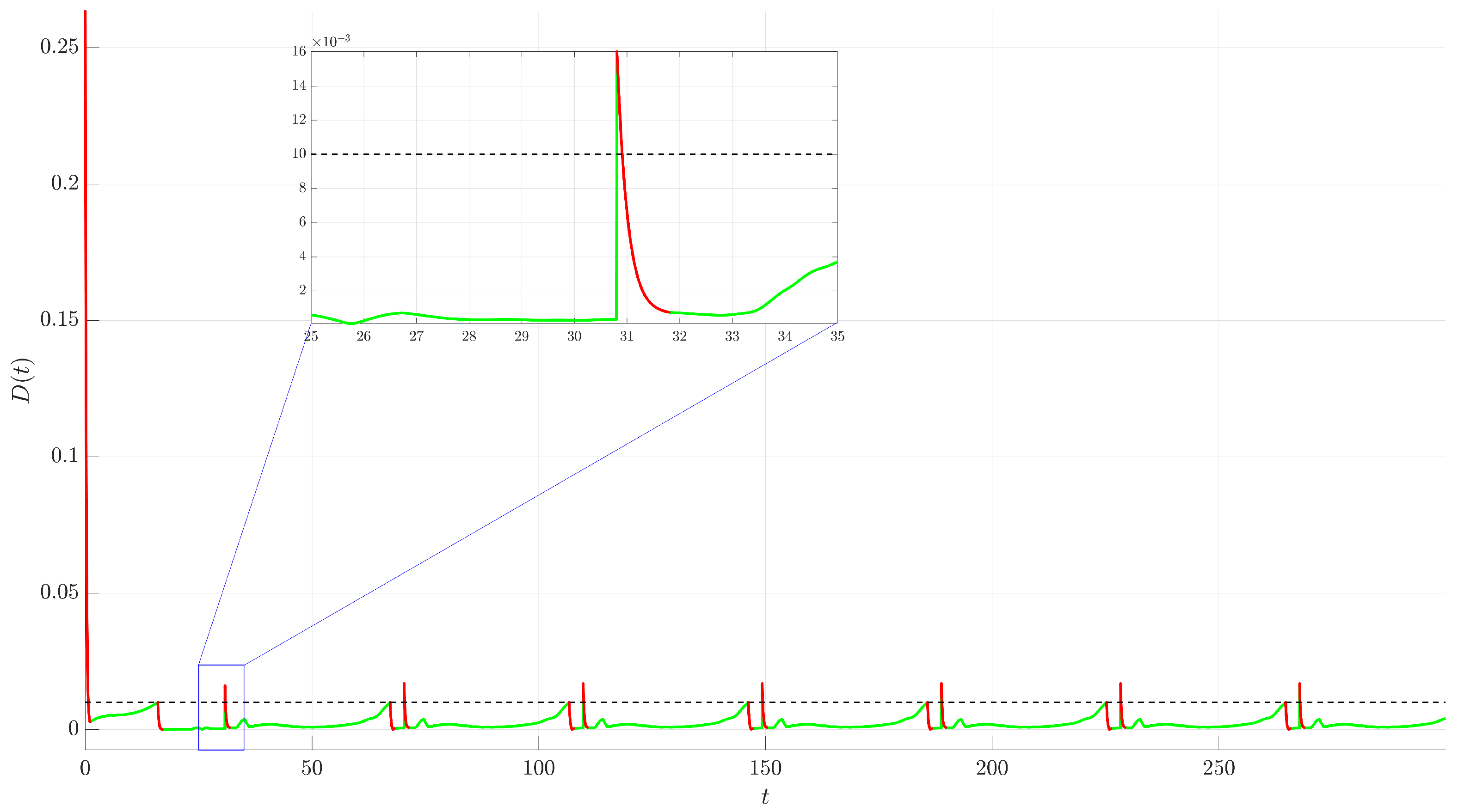The stabilization is also evident in the phase portrait and its projections shown in Figure 4. The controlled trajectory (red) rapidly converges towards the target UPO (dashed black line). The convergence is quantified by the Euclidean distance $D\left(t\right)=\parallel \mathbf{x}\left(t\right)-{\mathbf{x}}^{\left(UPO\right)}\left(t\right)\parallel$ between the controlled state and the UPO, depicted in Figure 5. The distance sharply decreases after control activation at $t=0$ and remains close to zero thereafter.

From a clinical perspective, this continuous control method represents an idealized therapeutic regimen, analogous to a continuous infusion of a therapeutic agent. While this strategy provides a valuable theoretical benchmark for stabilization, its inherent requirement for persistent intervention poses significant practical limitations. Continuous application can be undesirable or infeasible due to cumulative toxicity, patient discomfort, economic burden, and the high selective pressure it places on cancer cells, which can accelerate the development of drug resistance.

These considerations motivate the investigation of intermittent control strategies wherein the control mechanism is applied discontinuously and activated or deactivated based on the system’s stabilization status. The following subsections, therefore, explore intermittent control strategies designed to maintain stability while significantly reducing the total control effort.

3.2. Intermittent External Force Control

The intermittent approach applies the same control force as in (3) but switches it on or off based on the system’s proximity to the target UPO. The control activation is determined by the distance $D\left(t\right)=\parallel \mathbf{x}\left(t\right)-{\mathbf{x}}^{\left(UPO\right)}\left(t\right)\parallel$:

$$\mathbf{F}\left(t\right)=\left\{\begin{array}{cc}K\left({\mathbf{x}}^{\left(UPO\right)}\left(t\right)-\mathbf{x}\left(t\right)\right),\hfill & \mathrm{if}D\left(t\right)>\epsilon \hfill \\ \mathbf{0},\hfill & \mathrm{if}D\left(t\right)\le \epsilon \hfill \end{array}\right.,$$

(7)

where $\epsilon >0$ is the activation threshold. The control activates only when the system’s trajectory is beyond the $\epsilon$-neighborhood of the UPO. The goal is to maintain the trajectory near the UPO using minimal control action. The simulations shown use $K=5$ and $\epsilon =0.01$. The behavior under this strategy is illustrated in Figure 6, Figure 7, Figure 8 and Figure 9.

Figure 6 shows the time evolution of the state variables. Unlike the continuous case, the trajectory now alternates between controlled segments (red, when $D\left(t\right)>\epsilon$) and uncontrolled segments (green, when $D\left(t\right)\le \epsilon$). The system is corrected when it strays too far from the UPO and is allowed to evolve according to its natural dynamics once it is within the prescribed tolerance. This demonstrates the on–off nature of the control.

Figure 7 provides a zoomed-in view of the time series from Figure 6. This magnification reveals a potential issue with this simple switching logic: chattering. As the trajectory oscillates around the boundary $D\left(t\right)=\epsilon$, the control rapidly switches on and off. This high-frequency switching might be undesirable or damaging in practical implementations.

The phase portrait and its projections are shown in Figure 8. The trajectory remains confined near the target UPO (dashed black line), indicating successful stabilization. The alternating red and green segments highlight the periods of active control and free evolution, respectively.

Figure 9 plots the distance $D\left(t\right)$ and clearly shows the switching dynamics. The control activates (red segments) when $D\left(t\right)$ exceeds $\epsilon =0.01$ (dashed black line) and deactivates (green segments) when $D\left(t\right)$ drops below $\epsilon$. The inset highlights the chattering phenomenon through which the distance frequently crosses the threshold, leading to rapid control switching.

The therapeutic interpretation of this strategy is that of a reactive or on-demand therapy, where treatment is initiated only when the tumor burden crosses a specific threshold. However, the chattering phenomenon revealed in the analysis (Figure 9) corresponds to a clinically unfeasible scenario. It would imply starting and stopping a therapeutic intervention at an extremely high frequency, which is not only impractical to administer but could also lead to unpredictable drug concentrations in the patient, potentially fostering the evolution of resistant cancer cell populations. This highlights the need for a control logic that prevents such rapid switching.

3.3. Intermittent Control with Minimum Activation Duration

To address the chattering issue observed in the simple state-dependent intermittent strategy, a modification is introduced that enforces a minimum duration for which the control must remain active once triggered. This strategy aims to prevent rapid switching by ensuring the control acts for a substantial period once turned on, allowing the system state to move well within the $\epsilon$-neighborhood before deactivation is considered. The control force is modulated by a switching signal $\sigma \left(t\right)\in \{0,1\}$, such that the overall control input is as follows:

$$\mathbf{F}\left(t\right)=\sigma \left(t\right)·K\left({\mathbf{x}}^{\left(UPO\right)}\left(t\right)-\mathbf{x}\left(t\right)\right).$$

(8)

The switching signal $\sigma \left(t\right)$ is governed by a logic designed to prevent rapid toggling. The control activates ($\sigma \left(t\right)$ switches from 0 to 1) at time $t_{\mathrm{act}}$ when the distance, $D\left(t\right)$, first exceeds the threshold $\epsilon$. Once active, the control is guaranteed to remain on for a minimum duration of $T_{\min }$. Deactivation ($\sigma \left(t\right)$ switching from 1 to 0) is only permitted when two conditions are met simultaneously: the minimum activation time has elapsed ($t\ge t_{\mathrm{act}}+T_{\min }$), and the system’s trajectory has returned to the desired neighborhood ($D\left(t\right)\le \epsilon$). If these conditions for deactivation are not met after the minimum time, the control remains on until the trajectory is successfully stabilized within the $\epsilon$-neighborhood. For the simulations, the parameter values $K=5$, $\epsilon =0.01$, and $T_{\min }=1$ were used. The results of this modified strategy are shown in Figure 10, Figure 11, Figure 12 and Figure 13.

Figure 10 displays the time evolution of the state variables. The trajectory alternates between controlled (red, $\sigma \left(t\right)=1$) and uncontrolled (green, $\sigma \left(t\right)=0$) segments. Compared to Figure 6, the red segments are visibly longer and less frequent.

The zoomed-in view in Figure 11 shows the effect of the minimum activation duration. Once control activates (start of red segment), it remains on for at least $T_{\min }=1$. Even if $D\left(t\right)$ drops below $\epsilon$ during this initial period, the control persists. Deactivation (start of green segment) only occurs after $t\ge t_{\mathrm{act}}+T_{\min }$ and $D\left(t\right)\le \epsilon$. This effectively eliminates the high-frequency chattering seen previously.

The phase portrait and its projections in Figure 12 show the trajectory successfully stabilized near the target UPO (dashed black line). Again, the switching between controlled (red) and uncontrolled (green) dynamics is less frequent than in Figure 8.

Figure 13 plots the distance $D\left(t\right)$. When $D\left(t\right)$ exceeds $\epsilon =0.01$ (dashed black line), control activates (red segment begins) and stays active for at least $T_{\min }=1$. If $D\left(t\right)$ is still above $\epsilon$ when $t=t_{\mathrm{act}}+T_{\min }$, the control remains on until $D\left(t\right)$ eventually drops below or equals $\epsilon$. The inset demonstrates the successful suppression of chattering; the distance remains below $\epsilon$ for significant periods before control is potentially reactivated.

This modified strategy has a much more direct and realistic clinical analogue. The introduction of the minimum activation time directly corresponds to the administration of a standard treatment cycle. In clinical practice, therapies are prescribed over a defined period (e.g., several days or weeks) and are not stopped instantaneously based on an immediate biological response. This control method, therefore, represents a treat-and-wait strategy where a full course of therapy is initiated when the tumor burden grows beyond a set limit. By eliminating chattering, this approach models a far more practical approach to cancer management.

3.4. Adaptive Intermittent Control

Building upon the chatter-suppressed intermittent strategy, this section introduces an adaptive mechanism for the control parameter, K, allowing the system to automatically adjust the control strength. The control force is given as follows:

$$\mathbf{F}\left(t\right)=\sigma \left(t\right)·K\left(t\right)\left({\mathbf{x}}^{\left(UPO\right)}\left(t\right)-\mathbf{x}\left(t\right)\right),$$

(9)

where $K\left(t\right)$ is the time-varying adaptive control gain, and $\sigma \left(t\right)$ is the chatter-suppressing switching signal from Section 3.3.

The main difference lies in the adaptation law for the gain, $K\left(t\right)$, which consists of two parts: a continuous update rule applied when the control is active, and a discrete reset rule applied at the moment of deactivation. When the control is active ($\sigma \left(t\right)=1$), the gain, $K\left(t\right)$, evolves according to the differential equation:

$$\frac{\mathrm{d}K}{\mathrm{d}t}=\gamma \left(D\left(t\right)-\epsilon \right).$$

(10)

This law increases the gain when the trajectory is outside the $\epsilon$-neighborhood and decreases it when the trajectory is inside, dynamically tuning the control strength based on performance. At the instant the control deactivates (i.e., when $\sigma \left(t\right)$ switches from 1 to 0), the gain is immediately reset to its initial value $K\left(0\right)$. During the subsequent inactive period ($\sigma \left(t\right)=0$), the gain remains constant at this reset value until the next activation.

For the simulations, the same switching parameters $\epsilon =0.01$ and $T_{\min }=1$ were used, alongside an adaptation rate $\gamma =100$ and an initial gain $K\left(0\right)=5$.

The performance of the adaptive strategy is illustrated in Figure 14, Figure 15, Figure 16 and Figure 17. The time evolution of the state variables (Figure 14 and Figure 15), phase portrait and its projections (Figure 16), and distance from the UPO (Figure 17) demonstrate that the system is successfully stabilized. The resulting dynamics appear qualitatively similar to the non-adaptive case from Section 3.3, indicating that stability is robustly maintained even as the control gain varies.

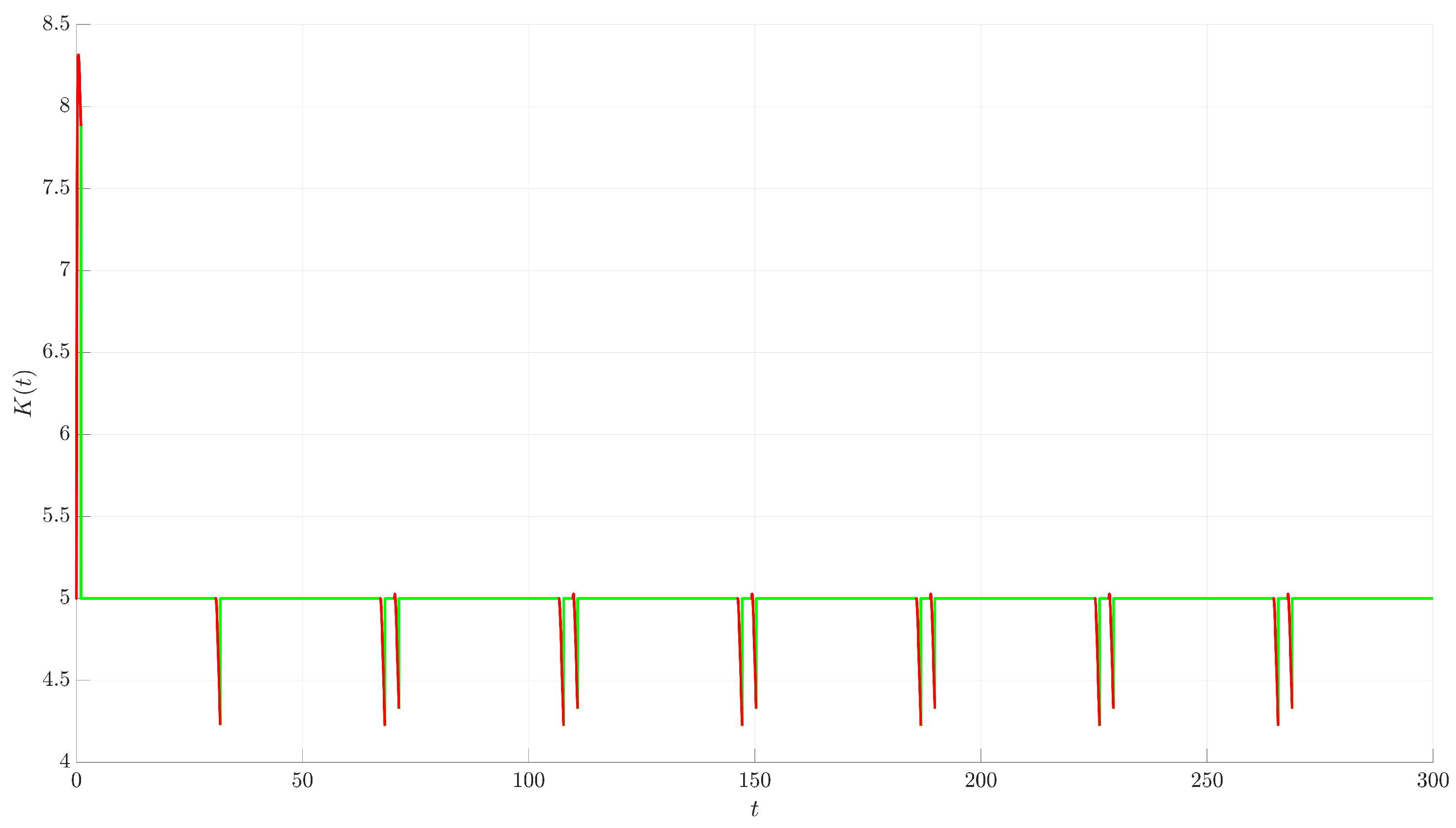
The evolution of $K\left(t\right)$ is depicted in Figure 18. Starting at $K\left(0\right)=5$, the parameter is adjusted dynamically during the control-on periods (red segments). When control activates because $D\left(t\right)>\epsilon$, $K\left(t\right)$ initially increases. If control is effective and $D\left(t\right)$ drops below $\epsilon$ while $\sigma \left(t\right)$ is still 1 (due to $T_{\min }$), $K\left(t\right)$ decreases. This adaptive strategy successfully stabilizes the system while automatically modulating the control based on performance relative to the threshold $\epsilon$.

This control strategy represents the most sophisticated and clinically forward-thinking technique investigated in this study—adaptive therapy. This approach moves beyond simple on–off switching based on a fixed-dosage plan. By allowing the control gain $K\left(t\right)$ to vary in response to the system’s error, the strategy models a treatment where the dosage or intensity is actively modulated during the treatment cycle based on the patient’s observed response. For example, a less-than-optimal response could trigger an increase in dosage, while a strong response could allow for a dose reduction to mitigate side effects. This method directly aligns with the goals of personalized medicine, aiming to steer the tumor dynamics using the minimum necessary intervention to manage toxicity and delay the onset of resistance.

3.5. Comparative Analysis of Control Strategies

To provide a comprehensive evaluation, this section compares the performance of the four implemented control strategies. The goal is to quantify the trade-offs between stabilization accuracy and the required control effort, highlighting the distinct advantages and disadvantages of each method.

The comparison is based on a simulation run for each strategy over a total duration of $T_{sim}=300$ time units, starting from the same initial condition $\mathbf{x}\left(0\right)=(0.2,0.2,0.1)$. Performance is quantified using three key metrics, summarized in

Table 1. Comparison of control strategy performance.

Control Strategy	Total Distance	Control-On Time (%)	Total Impulse
Continuous control	21.54	100.00%	107.71
Intermittent control	141.19	1.32%	42.71
Intermittent with min. activation	70.62	5.00%	47.79
Adaptive intermittent control	63.19	4.67%	46.23

. The first, total distance, is the time integral of the Euclidean distance, $D\left(t\right)=\parallel \mathbf{x}\left(t\right)-{\mathbf{x}}^{\left(UPO\right)}\left(t\right)\parallel$, which represents the accumulated tracking error over the entire simulation. The second metric, control-on time, is the percentage of the total simulation time during which the control force was active, quantifying the temporal burden of the control. The third, total control impulse, is the time integral of the magnitude of the control force vector, serving as a measure of the total energy or resources expended by the controller.

An analysis of the results in Table 1 reveals a clear hierarchy of performance and efficiency. The continuous control acts as a performance benchmark. As expected, it achieves the highest precision with the lowest total distance. However, this comes at the maximum possible cost, with a control-on time of 100% and the highest total control impulse.

Switching to the simple intermittent control strategy results in a dramatic reduction in control effort, as evidenced by its minimal control-on time. This efficiency, however, is gained at the expense of performance, as the total distance increases significantly. This method also suffers from the chattering phenomenon, where the controller rapidly switches on and off near the boundary of the activation threshold.

The intermittent control with minimum activation duration successfully addresses these shortcomings. By eliminating chattering and ensuring that the control acts for a more substantial period once triggered, it cuts the total distance in half compared to the simple intermittent method. This significant improvement in accuracy comes with a slight increase in the control-on time.

Finally, the adaptive intermittent control demonstrates a further refinement. It achieves the best performance among the intermittent strategies, with the lowest total distance and total control impulse in this category. Its primary advantage is its ability to achieve this robust performance without requiring manual tuning of the control gain, K. It automatically adjusts the gain based on system performance, finding an effective balance dynamically.

It is crucial to emphasize that the intermittent and adaptive strategies introduce additional parameters, which act as new degrees of freedom for tuning the controller. The results presented in Table 1 correspond to the specific parameter values used earlier in this study, namely an activation threshold of $\epsilon =0.01$, a minimum activation time of $T_{\min }=1$, an initial gain of $K\left(0\right)=5$, and an adaptation rate of $\gamma =100$. A different choice of these parameters would lead to different quantitative results; for instance, a larger threshold $\epsilon$ would further reduce control effort but likely increase the tracking error. The purpose of this study was not to perform an exhaustive parameter optimization but, rather, to introduce and compare the fundamental mechanics and inherent trade-offs of these distinct control frameworks. For any practical application, a careful tuning of these parameters would be a necessary subsequent step.

4. Conclusions

This study implemented and compared four distinct external force control strategies for suppressing the chaotic dynamics of a well-established three-dimensional cancer model [34]. The objective was to stabilize a target UPO embedded within the system’s strange attractor, thereby transforming the unpredictable, chaotic behavior into a regular, periodic dynamic.

The investigation first established a baseline using continuous control, which, while highly precise in tracking the target UPO, required constant intervention and the largest control effort. In contrast, a simple intermittent control strategy drastically reduced the control effort, but at the cost of significantly lower accuracy and the introduction of high-frequency chattering. To address this, a modified intermittent controller incorporating a minimum activation duration was introduced. This method successfully eliminated chattering and substantially improved tracking performance, demonstrating a favorable balance between control accuracy and efficiency.

The most promising results were obtained with the adaptive intermittent control strategy. This approach not only matched the improved performance of the chatter-free method but also achieved the lowest total control impulse among the intermittent strategies. Its principal advantage lies in its ability to dynamically tune the control gain, showcasing a robust mechanism for self-optimization. The findings underscore that both chatter-suppressed and adaptive intermittent control offer more practical and efficient alternatives to continuous intervention, which is an important consideration for therapeutic applications. By minimizing the duration and intensity of the intervention, these strategies could potentially lead to treatments with fewer side effects, lower economic costs, and a reduced likelihood of developing treatment resistance, making them more practical and sustainable for patient care.

The scope of this work was a comparative analysis of the control frameworks, rather than an exhaustive optimization of their parameters. Future research should focus on a systematic investigation of the parameter space (e.g., $\epsilon$, $T_{\min }$, $\gamma$) to formally optimize the trade-off between control effort and stabilization accuracy. Further valuable extensions could include applying these adaptive and intermittent strategies to more complex cancer models that incorporate additional biological factors, such as pharmacokinetics or different immune cell populations. Finally, investigating the robustness of these controllers to system noise and parameter uncertainty, which are inherent to all biological systems, would be a critical step toward assessing their potential for real-world application.

References

1. Shutaywi, M.; Shah, Z.; Jan, R. A robust study of the dynamics of tumor–immune interaction for public health via fractional framework. Eur. Phys. J. Spec. Top. 2024, 1–20. [Google Scholar] [CrossRef]
2. Li, J.; Tan, X.; Wu, W.; Liu, X. Chaotic dynamics and optimal therapeutic strategies for Caputo fractional tumor immune model in combination therapy. Chaos Interdiscip. J. Nonlinear Sci. 2024, 34, 113113. [Google Scholar] [CrossRef]
3. Tutsoy, O.; Barkana, D.E. Model free adaptive control of the under-actuated robot manipulator with the chaotic dynamics. ISA Trans. 2021, 118, 106–115. [Google Scholar] [CrossRef]
4. Guo, F.; Zhang, H.; Yu, H. Dynamic Properties and Chaos Control of a High Dimensional Double Rotor Model. Autom. Control Comput. Sci. 2024, 58, 227–236. [Google Scholar]
5. Kumar, S.; Matouk, A.E.; Chaudhary, H.; Kant, S. Control and synchronization of fractional-order chaotic satellite systems using feedback and adaptive control techniques. Int. J. Adapt. Control Signal Process. 2021, 35, 484–497. [Google Scholar] [CrossRef]
6. Zhou, Z.X.; Ren, H.P.; Grebogi, C. Bi-directional impulse chaos control in crystal growth. Chaos Interdiscip. J. Nonlinear Sci. 2021, 31, 053106. [Google Scholar] [CrossRef]
7. Zhu, G.L.; Hu, C.S.; Wu, Y.; Lü, X.Y. Cavity optomechanical chaos. Fundam. Res. 2023, 3, 63–74. [Google Scholar] [CrossRef]
8. Navarro-Urrios, D.; Capuj, N.E.; Colombano, M.F.; García, P.D.; Sledzinska, M.; Alzina, F.; Griol, A.; Martínez, A.; Sotomayor-Torres, C.M. Nonlinear dynamics and chaos in an optomechanical beam. Nat. Commun. 2017, 8, 14965. [Google Scholar] [CrossRef]
9. Zainol, Z.; Teh, J.S.; Alawida, M. An FPP-resistant SVD-based image watermarking scheme based on chaotic control. Alex. Eng. J. 2022, 61, 5713–5734. [Google Scholar]
10. Yousef, A.; Rida, S.; Ali, H.; Zaki, A. Stability, co-dimension two bifurcations and chaos control of a host-parasitoid model with mutual interference. Chaos Solitons Fractals 2023, 166, 112923. [Google Scholar] [CrossRef]
11. Elmacı, D.; Kangalgil, F. Complex Dynamics of a Discrete Prey–Predator Model Exposing to Harvesting and Allee Effect on the Prey Species with Chaos Control. Int. J. Bifurc. Chaos 2024, 34, 2450114. [Google Scholar] [CrossRef]
12. Abbasi, M.A. Analyzing global patterns, stability, bifurcation, and chaos control of an ecological model. Int. J. Dyn. Control 2025, 13, 151. [Google Scholar] [CrossRef]
13. Lilienkamp, T.; Parlitz, U.; Luther, S. Taming cardiac arrhythmias: Terminating spiral wave chaos by adaptive deceleration pacing. Chaos Interdiscip. J. Nonlinear Sci. 2022, 32, 121105. [Google Scholar] [CrossRef]
14. Qu, Z. Chaos in the genesis and maintenance of cardiac arrhythmias. Prog. Biophys. Mol. Biol. 2011, 105, 247–257. [Google Scholar] [CrossRef]
15. Farman, M.; Nisar, K.S.; Shehzad, A.; Baleanu, D.; Amjad, A.; Sultan, F. Computational analysis and chaos control of the fractional order syphilis disease model through modeling. Ain Shams Eng. J. 2024, 15, 102743. [Google Scholar] [CrossRef]
16. Yao, Z.; Sun, K.; He, S. Dynamics of fractional-order chaotic rocard relaxation econometric system. Int. J. Bifurc. Chaos 2022, 32, 2250195. [Google Scholar] [CrossRef]
17. Gecow, A.; Iantovics, L.B.; Tez, M. Cancer and chaos and the complex network model of a multicellular organism. Biology 2022, 11, 1317. [Google Scholar] [CrossRef]
18. Ott, E. Chaos in Dynamical Systems; Cambridge University Press: Cambridge, UK, 2002. [Google Scholar]
19. Kuznetsov, V.A.; Makalkin, I.A.; Taylor, M.A.; Perelson, A.S. Nonlinear dynamics of immunogenic tumors: Parameter estimation and global bifurcation analysis. Bull. Math. Biol. 1994, 56, 295–321. [Google Scholar] [CrossRef] [PubMed]
20. Weinberg, R.A. How cancer arises. Sci. Am. 1996, 275, 62–70. [Google Scholar] [CrossRef] [PubMed]
21. Waliszewski, P.; Molski, M.; Konarski, J. On the holistic approach in cellular and cancer biology: Nonlinearity, complexity, and quasi-determinism of the dynamic cellular network. J. Surg. Oncol. 1998, 68, 70–78. [Google Scholar] [CrossRef]
22. Moghtadaei, M.; Hashemi Golpayegani, M.R.; Malekzadeh, R. Periodic and chaotic dynamics in a map-based model of tumor–immune interaction. J. Theor. Biol. 2013, 334, 130–140. [Google Scholar] [CrossRef]
23. Khajanchi, S. Chaotic dynamics of a delayed tumor–immune interaction model. Int. J. Biomath. 2020, 13, 2050009. [Google Scholar] [CrossRef]
24. Ch-Chaoui, M.; Mokni, K. Asymptotic analysis of an integro-differential system modeling the blow up of cancer cells under the immune response. J. Appl. Anal. Comput. 2022, 12, 1763–1785. [Google Scholar] [CrossRef] [PubMed]
25. Uthamacumaran, A.; Zenil, H. A review of mathematical and computational methods in cancer dynamics. Front. Oncol. 2022, 12, 850731. [Google Scholar] [CrossRef]
26. Das, S.; Mandal, G.; Dutta, S.; Guin, L.N.; Chakravarty, K. Analysis and regulation of chaos dynamics in a cancer model through chemotherapeutic intervention and immune system augmentation. Int. J. Dyn. Control 2024, 12, 3884–3907. [Google Scholar] [CrossRef]
27. Jiao, H.; Shen, Q.; Shi, Y.; Shi, P. Adaptive tracking control for uncertain cancer-tumor-immune systems. IEEE/ACM Trans. Comput. Biol. Bioinform. 2020, 18, 2753–2758. [Google Scholar] [CrossRef]
28. El-Gohary, A.; Alwasel, I. The chaos and optimal control of cancer model with complete unknown parameters. Chaos Solitons Fractals 2009, 42, 2865–2874. [Google Scholar] [CrossRef]
29. El-Gohary, A. Chaos and optimal control of cancer self-remission and tumor system steady states. Chaos Solitons Fractals 2008, 37, 1305–1316. [Google Scholar] [CrossRef]
30. Das, P.; Das, S.; Das, P.; Rihan, F.A.; Uzuntarla, M.; Ghosh, D. Optimal control strategy for cancer remission using combinatorial therapy: A mathematical model-based approach. Chaos Solitons Fractals 2021, 145, 110789. [Google Scholar] [CrossRef]
31. Mohammadi, S.; Hejazi, S.R. Using particle swarm optimization and genetic algorithms for optimal control of non-linear fractional-order chaotic system of cancer cells. Math. Comput. Simul. 2023, 206, 538–560. [Google Scholar] [CrossRef]
32. Shahzad, M. Chaos control in three dimensional cancer model by state space exact linearization based on lie algebra. Mathematics 2016, 4, 33. [Google Scholar] [CrossRef]
33. Gurcan, F.; Kartal, S. Chaos and its control in a discretized fractional order tumor-immune system model with benign and malignant case. J. Appl. Math. Comput. 2025, 1–29. [Google Scholar] [CrossRef]
34. Itik, M.; Banks, S.P. Chaos in a three-dimensional cancer model. Int. J. Bifurc. Chaos 2010, 20, 71–79. [Google Scholar] [CrossRef]
35. Ch-Chaoui, M.; Mokni, K. A multi-parameter bifurcation analysis of a prey–predator model incorporating the prey Allee effect and predator-induced fear. Nonlinear Dyn. 2025, 113, 18879–18911. [Google Scholar] [CrossRef]
36. Pyragas, K. Continuous control of chaos by self-controlling feedback. Phys. Lett. A 1992, 170, 421–428. [Google Scholar] [CrossRef]
Figure 1. Chaotic attractor of the system (1) with parameter values a 12 = 1 , a 13 = 2.5 , a 21 = 1.5 , r 2 = 0.6 , a 31 = 0.2 , d 3 = 0.5 , r 3 = 4.5 , and k 3 = 1 . The 3D phase portrait of the chaotic attractor and its projections onto the x 1 x 2 , x 1 x 3 , and x 2 x 3 planes are shown in the four panels, respectively. Blue dot corresponds to the initial condition x 1 = 0.2 , x 2 = 0.2 , x 3 = 0.1 .
Mca 30 00081 g001
Figure 2. The 3D phase portrait of the target UPO and its projections onto the x 1 x 2 , x 1 x 3 , and x 2 x 3 planes. The period of this orbit is T ( U P O ) 39.5011 , and a point on the orbit is approximately x ( U P O ) ( 0 ) = ( 0.5 , 0.2850 , 0.0067 ) . The full reference trajectory is obtained by numerically integrating system (1) over one period from this initial condition.
Mca 30 00081 g002
Figure 3. Time evolution of state variables under continuous external force control applied to system (1). Green lines correspond to the chaotic trajectory ( x ( 0 ) = ( 0.2 , 0.2 , 0.1 ) ). Red lines correspond to the trajectory under continuous control (4) with K = 5 , activated at t = 0 .
Mca 30 00081 g003
Figure 4. The 3D phase portrait and its projections under continuous external force control applied to system (1). The green line corresponds to the chaotic trajectory. The red line shows the trajectory under continuous control (4) with K = 5 , activated at t = 0 . The blue dot depicts the initial condition x ( 0 ) = ( 0.2 , 0.2 , 0.1 ) . The dashed black line is the target UPO.
Mca 30 00081 g004
Figure 5. Time evolution of the Euclidean distance D ( t ) = x ( t ) x ( U P O ) ( t ) between the controlled trajectory and the target UPO under continuous external force control ( K = 5 , activated at t = 0 ).
Mca 30 00081 g005
Figure 6. Time evolution of state variables under intermittent external force control applied to system (1). Control parameters are K = 5 and ε = 0.01 . Red segments indicate periods when control is active ( D ( t ) > ε ). Green segments correspond to periods when control is inactive ( D ( t ) ε ).
Mca 30 00081 g006
Figure 7. Zoomed-in view of Figure 6. The red segments (control is active) and green segments (control is inactive) alternate frequently as the trajectory oscillates near the switching threshold D ( t ) = ε , illustrating chattering.
Mca 30 00081 g007
Figure 8. The 3D phase portrait and its projections under intermittent external force control ( K = 5 , ε = 0.01 ). The red segments indicate periods when control is active ( D ( t ) > ε ). The green segments correspond to periods when control is inactive ( D ( t ) ε ). The dashed black line corresponds to the target UPO. The blue dot depicts the initial condition x ( 0 ) = ( 0.2 , 0.2 , 0.1 ) .
Mca 30 00081 g008
Figure 9. Time evolution of the distance D ( t ) under intermittent external force control ( K = 5 , ε = 0.01 ). The red segments indicate periods when control is active ( D ( t ) > ε ). The green segments correspond to periods when control is inactive ( D ( t ) ε ). The black dashed line represents the activation threshold ε = 0.01 . The blue rectangle highlights a zoomed-in region where chattering is observed. The inset shows a magnified view of this region, illustrating the chattering phenomenon..
Mca 30 00081 g009
Figure 10. Time evolution of state variables under intermittent control with minimum activation duration ( K = 5 , ε = 0.01 , T min = 1 ). Red segments indicate periods when control is active ( σ ( t ) = 1 ). Green segments correspond to inactive control periods ( σ ( t ) = 0 ). Control activates when D ( t ) > ε and remains active for at least T min = 1 , deactivating only when D ( t ) ε afterwards.
Mca 30 00081 g010
Figure 11. Zoomed-in view of Figure 10. Red segments indicate periods when control is active ( σ ( t ) = 1 ). Green segments correspond to inactive control periods ( σ ( t ) = 0 ). Red segments persist for at least T min = 1 after activation, and potentially longer, until D ( t ) ε . Chattering is effectively suppressed.
Mca 30 00081 g011
Figure 12. The 3D phase portrait and its projections under intermittent control with minimum activation duration ( K = 5 , ε = 0.01 , T min = 1 ). The red segments indicate periods when control is active. The green segments correspond to periods when control is inactive. The dashed black line corresponds to the target UPO. The blue dot depicts the initial condition x ( 0 ) = ( 0.2 , 0.2 , 0.1 ) .
Mca 30 00081 g012
Figure 13. Time evolution of the distance D ( t ) under intermittent control with minimum activation duration ( K = 5 , ε = 0.01 , T min = 1 ). The red segments denote active control, and the green segments denote inactive control. The black dashed line is the threshold ε . Control activates when D ( t ) > ε and deactivates only when t t act + T min and D ( t ) ε . The inset (zoomed-in view of the blue rectangle) confirms the absence of chattering.
Mca 30 00081 g013
Figure 14. Time evolution of state variables under adaptive intermittent control (9) and (10) with switching parameters ε = 0.01 , T min = 1 , adaptation rate γ = 100 , and initial gain K ( 0 ) = 5 . Red segments indicate active control periods (with adaptive gain K ( t ) ), and green segments indicate inactive periods.
Mca 30 00081 g014
Figure 15. Zoomed-in view of Figure 14. Red segments indicate active control periods (with adaptive gain K ( t ) ), and green segments indicate inactive periods.
Mca 30 00081 g015
Figure 16. The 3D phase portrait and its projections under adaptive intermittent control ( ε = 0.01 , T min = 1 , γ = 100 , K ( 0 ) = 5 ). The red segments indicate periods when control is active. The green segments correspond to periods when control is inactive. The dashed black line corresponds to the target UPO. The blue dot depicts the initial condition x ( 0 ) = ( 0.2 , 0.2 , 0.1 ) .
Mca 30 00081 g016
Figure 17. Time evolution of the distance, D ( t ) , under adaptive intermittent control ( ε = 0.01 , T min = 1 , γ = 100 , K ( 0 ) = 5 ). The red segments denote active control, and the green segments denote inactive control. The black dashed line is the threshold ε . The inset shows a magnified view of the area outlined by the blue rectangle.
Mca 30 00081 g017
Figure 18. Time evolution of the adaptive control gain K ( t ) (10) with γ = 100 and initial gain K ( 0 ) = 5 . The red segments indicate periods when control is active and K ( t ) adapts. The green segments correspond to inactive periods. The gain K ( t ) is reset to K ( 0 ) = 5 at the beginning of each inactive period and held constant until the next activation.
Mca 30 00081 g018