Deciding on the Regularity of a Planar Coons Map

Abstract

We consider the construction of a regular map from the unit square to a general four-sided domain, a problem that arises in several applications, e.g., in the numerical solution of integral equations or when dealing with trimmed surfaces in CAD. In our approach, we consider the problem in as general a form as possible, which means that initially no assumptions are made about the type of mathematical representation of the boundary curves. This approach becomes possible by using planar Coons maps to describe the parameterization. We show that the regularity of a Coons map depends both on the waviness and the similarity of the boundary curves. Constraining these properties allows us to formulate sufficient conditions for regularity and to specify special cases in which the regularity of the Coons map is obvious. For the case of polynomial boundary curves, we present a regularity criterion that is both necessary and sufficient and can thus be used to characterize regular polynomial mappings. Our decision algorithm implements this criterion and provides a powerful tool not only for deciding the regularity of a given Coons map, but also for determining the transition between a regular and a non-regular Coons map depending on the curvature of the boundary curves.

1. Introduction

In Computer-Aided Geometric Design (CAGD), a Coons patch refers to a particular representation of a parametric surface $x:{[0, 1]}^2\to {\mathbf{R}}^3$ that is fitted into a topologically four-sided loop of space curves [1,2]. If the interpolation curves lie in a plane, the Coons patch establishes a map from ${[0, 1]}^2$ to a planar domain bounded by four potentially curved sides. Therefore, Gordon already proposed that a planar Coons patch (hereafter referred to as a Coons map) could be used for creating planar reparametrizations, which are essential for various applications, including CAGD, mesh generation, and numerical integration [3,4,5].

In CAGD, reparametrizations are needed for various tasks, but especially in the context of “surface trimming”. Trimming a model means removing parts of an existing design. This is carrjed kht by specifying “trimming curves” in the parameter domain of a tensor product surface to identify the part of the design to be removed. The introduction of trimmed surfaces has significantly extended the ability of CAD systems to represent complex shapes [6] and the designs of most industrial products contain trimmed surfaces. Figure 1 shows an example of the use of trimmed surfaces in car body design; further examples can be found in [7].

However, trimming results in parameter domains of non-rectangular shape, often even bounded by curved lines. Thus, a trimmed surface generally cannot be represented as a polynomial tensor product patch defined on a rectangular parameter domain. A popular approach to overcome this problem is to approximate the trimmed surface by a collection of tensor product patches. Another approach restores the standard quadratic form of the parameter domain using certain reparametrizations that allow the trimmed surface to be represented as a single Coons patch (see [8]). It has been shown in [5,8] that there are three different classes of reparametrizations that can be used for this task. Each of these reparametrizations can be represented as a Coons map, but the regularity of these maps depends on the waviness of the boundary curves, and methods are needed to check whether the regularity holds.

Regular reparametrizations also play an important role in the numerical solution of integral equations on closed surfaces. In the Wavelet Galerkin scheme, the surface must be decomposed into a collection of four-sided patches, each of which is a regular parametrization over the unit square (see, e.g., [9,10]).

In the context of mesh generation, Gordon had already proposed using a Coons map as a starting point and determining its regularity by visually inspecting the parameter lines. If regularity is not established, additional curves are specified within the domain and the resulting network of curves is interpolated using a more general transfinite interpolation scheme [4]. However, in general, it is not clear whether such a subdivision approach always provides geometrically valid, i.e., regular sub-elements. Mandad and Campen recently showed that planar domains with piecewise polynomial boundaries can always be tessellated into regular higher-order triangular elements [11]. For elements of non-triangular topology, however, it is still a problem to establish the regularity of the sub-elements and different algorithmic approaches are used. In isogeometric analysis, parameterizations of the computational domains are obtained by solving an optimization problem [12,13]. In [13], criteria that ensure regularity are included as constraints in the optimization. However, given the substantial computing time demands of such an approach, it has been proposed to perform an unconstrained optimization and subsequently check the regularity of the resulting mesh [12]. These methods rely on sufficient conditions for the regularity of planar parametrization that have been introduced in [14] and then generalized to higher dimensions, different topologies and maps that dynamically change over time [12,13,15]. However, relying solely on sufficient conditions carries the risk of over-restricting the tessellation. The only way to avoid this is to formulate a criterion that is both necessary and sufficient for regularity. The derivation of this criterion is the main result of this work and forms the basis of the algorithm for deciding regularity.

In our approach, we consider the problem in as general a form as possible and derive specific cases from the general consideration. This means that initially no assumptions are made about the type of mathematical representation of the boundary curves of a parameter range. This procedure becomes possible by using Coons surfaces to describe the parameterization.

In Section 3, we show that the regularity of the map depends both on the waviness and on the similarity of the boundary curves. Constraining these properties allows to formulate a sufficient condition for regularity (Theorem 1). This condition is then used to show that there are two special cases in which the regularity of the Coons map is obvious: (a) if the parameter domain is bounded by line segments, and (b) if opposite boundary curves are parallel translates of each other. These special cases, which frequently occur in applications, can be used to sort out parameterizations whose regularity does not need to be checked. An example of the application of this principle to the reparamerization of a trimmed surface is given in Section 4.

Starting with Section 4, we suppose that both the boundary curves and the blending functions are polynomials represented in Bézier form. This allows us to formulate the conditions of Theorem 1 as inequalities for the Bézier coefficients. The conditions for regularity presented in Theorem 2 are easy to evaluate and can be intuitively related to the geometry of the considered cases. This is demonstrated by analyzing a parametric example in which the shape of the boundary curves is controlled by a parameter. However, our experiments showed that the derived sufficiency conditions restrict the variation in the boundary curves more than necessary to obtain a regular Coons map. Less restrictive conditions are obtained by considering the determinant of the Jacobian of the Coons map in the Bézier representation. The regularity of the Coons map is assured if all Bézier coefficients of the Jacobian have the same sign (Theorem 3).

In Section 5, we apply a subdivision principle to formulate a criterion that is both necessary and sufficient for regularity. Theorem 4 states that a polynomial Coons map is regular if and only if it can be subdivided into submaps with equal signs of all Bézier coefficients of the Jacobians. Based on this theorem, we formulate an algorithm to decide on the regularity of a given Coons map $\mathbf{x}$ based on recursive adaptive subdivision. Sufficient criteria for non-regularity are used to abort the recursion.

In the presentation of our results, we refer to an example of the processing of trimmed surfaces to demonstrate the relevance of our method in CAGD. Certain shapes of parameter domains that appear in this example are considered prototypes of common cases. For these cases, we build parameterized models that allow us to modify the shape of the domain. In our experiments, we increase the shape parameter until the algorithm detects a non-regular Coons map. In this way, we precisely determine the transition between a regular and a non-regular Coons map in dependence on the shape parameter. This demonstrates that our method can be used by a CAD designer to determine existing margins and tolerances when defining decomposition curves. To visualize the quality of the parameterizations, we provide a plot of the scaled Jacobian function for the examples considered.

2. Transfinite Interpolation and Problem Setting

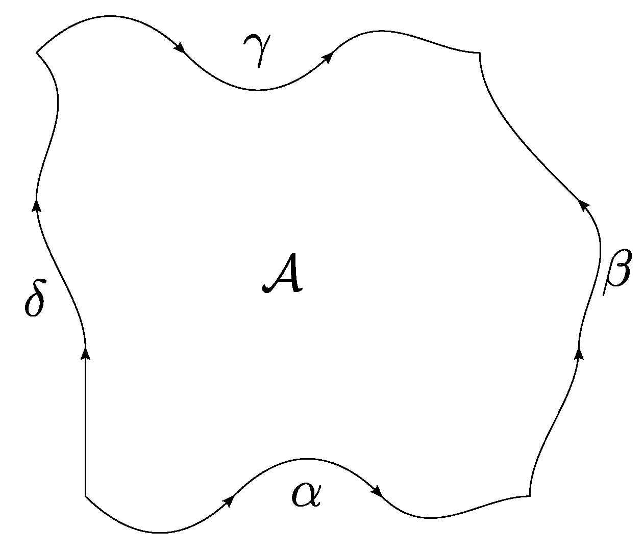
Let $\mathit{\alpha }$, $\mathit{\beta }$, $\mathit{\gamma }$, $\mathit{\delta }$$:[0, 1]⟶{\mathbf{R}}^2$ be four ${\mathcal{C}}^1[0, 1]$ curves that fulfill the compatibility conditions (see Figure 2) at the corners:

$$\mathit{\alpha }\left(0\right)=\mathit{\delta }\left(0\right),\mathit{\alpha }\left(1\right)=\mathit{\beta }\left(0\right),\mathit{\gamma }\left(0\right)=\mathit{\delta }\left(1\right),\mathit{\gamma }\left(1\right)=\mathit{\beta }\left(1\right).$$

(1)

We assume that besides the common points in (1), there are no further intersection points. Since our method of generating a map from the unit square to the four-sided domain $\mathcal{A}$ bounded by $\mathit{\alpha }$, $\mathit{\beta }$, $\mathit{\gamma }$, $\mathit{\delta }$ is based on transfinite interpolation, we briefly recall some basic facts about this technique. For more details, see [2,3,4,5].

We are interested in generating a map $\mathbf{x}$$:{[0, 1]}^2⟶{\mathbf{R}}^2$ such that the boundary of the image of $\mathbf{x}$ coincides with the given four curves:

$$\begin{array}{ccc}\mathbf{x}(u, 0)=\alpha \left(u\right)\hfill & & \mathbf{x}(u, 1)=\mathit{\gamma }\left(u\right)\forall u\in [0, 1]\hfill \\ \mathbf{x}(0, v)=\mathit{\delta }\left(v\right)\hfill & & \mathbf{x}(1, v)=\mathit{\beta }\left(v\right)\forall v\in [0, 1].\hfill \end{array}$$

(2)

This transfinite interpolation problem can be solved by a planar Coons map which is defined as follows. Let,

$$\begin{array}{ccc}\hfill \left(\mathcal{P}\mathbf{x}\right)(u, v)& :=& F_0\left(v\right)\mathbf{x}(u, 0)+F_1\left(v\right)\mathbf{x}(u, 1)\hfill \end{array}$$

(3)

$$\begin{array}{ccc}\hfill \left(\mathcal{Q}\mathbf{x}\right)(u, v)& :=& F_0\left(u\right)\mathbf{x}(0, v)+F_1\left(u\right)\mathbf{x}(1, v)\hfill \end{array}$$

(4)

where $F_0$ and $F_1$ denote two strictly monotone functions satisfying

$$F_i\left(j\right)={\delta }_{ij}i, j=0, 1\mathrm{and}{F}_0\left(t\right)+F_1\left(t\right)=1\forall t\in [0, 1].$$

(5)

Then, a Coons map $\mathbf{x}$ is defined by the relation

$$\mathbf{x}=\mathcal{P} \oplus \mathcal{Q}\left(\mathbf{x}\right)$$

(6)

with

$$\mathcal{P}\oplus \mathcal{Q}:=\mathcal{P}+\mathcal{Q}-\mathcal{P}\mathcal{Q}.$$

(7)

Inserting the definitions of the operators $\mathcal{P}$ and $\mathcal{Q}$ into (7), we obtain (see [16])

$$\begin{array}{ccc}\hfill \mathbf{x}(u, v)& :=& F_0\left(v\right)\mathbf{x}(u, 0)+F_1\left(v\right)\mathbf{x}(u, 1)+\hfill \\ & & F_0\left(u\right)\mathbf{x}(0, v)+F_1\left(u\right)\mathbf{x}(1, v)+\hfill \\ & & F_0\left(v\right)F_0\left(u\right)\mathbf{x}(0, 0)+F_1\left(v\right)F_0\left(u\right)\mathbf{x}(0, 1)+\hfill \\ & & F_0\left(v\right)F_1\left(u\right)\mathbf{x}(1, 0)+F_1\left(v\right)F_1\left(u\right)\mathbf{x}(1, 1).\hfill \end{array}$$

(8)

Writing this equation in matrix form yields

$$\mathbf{x}(u, v)=-{\left[\begin{array}{c}-1\\ F_0\left(u\right)\\ F_1\left(u\right)\end{array}\right]}^T\left[\begin{array}{ccc}\mathbf{0}& \mathbf{x}(u, 0)& \mathbf{x}(u, 1)\\ \mathbf{x}(0, v)& \mathbf{x}(0, 0)& \mathbf{x}(0, 1)\\ \mathbf{x}(1, v)& \mathbf{x}(1, 0)& \mathbf{x}(1, 1)\end{array}\right]\left[\begin{array}{c}-1\\ F_0\left(v\right)\\ F_1\left(v\right)\end{array}\right].$$

(9)

This construction is due to S. M. Coons [1] and it has been developed for free-form surface modeling. In that case, the given curves form a loop of space curves that is filled with a Coons patch. The Boolean sum character of a Coons patch has been discovered by W. Gordon [16].

The differentiability of a Coons map is guaranteed if all curves and blending functions involved are themselves differentiable. The blending functions $F_0$, $F_1$ can be chosen in several ways. Common choices involve linear blending functions:

$$F_0\left(t\right)=1-t,F_1\left(t\right)=t.$$

(10)

and cubic ones:

$$\begin{array}{ccc}\hfill F_0\left(t\right)& :=& 2t^3-3t^2+1=B_0^3\left(t\right)+B_1^3\left(t\right)\hfill \end{array}$$

(11)

$$\begin{array}{ccc}\hfill F_1\left(t\right)& :=& -2t^3+3t^2=B_2^3\left(t\right)+B_3^3\left(t\right).\hfill \end{array}$$

(12)

Here, $B_i^3\left(t\right)$$i=0,\dots , 3$ denotes the cubic Bezier functions.

Note, that the results presented in Section 3 are valid for a large variety of blending functions.

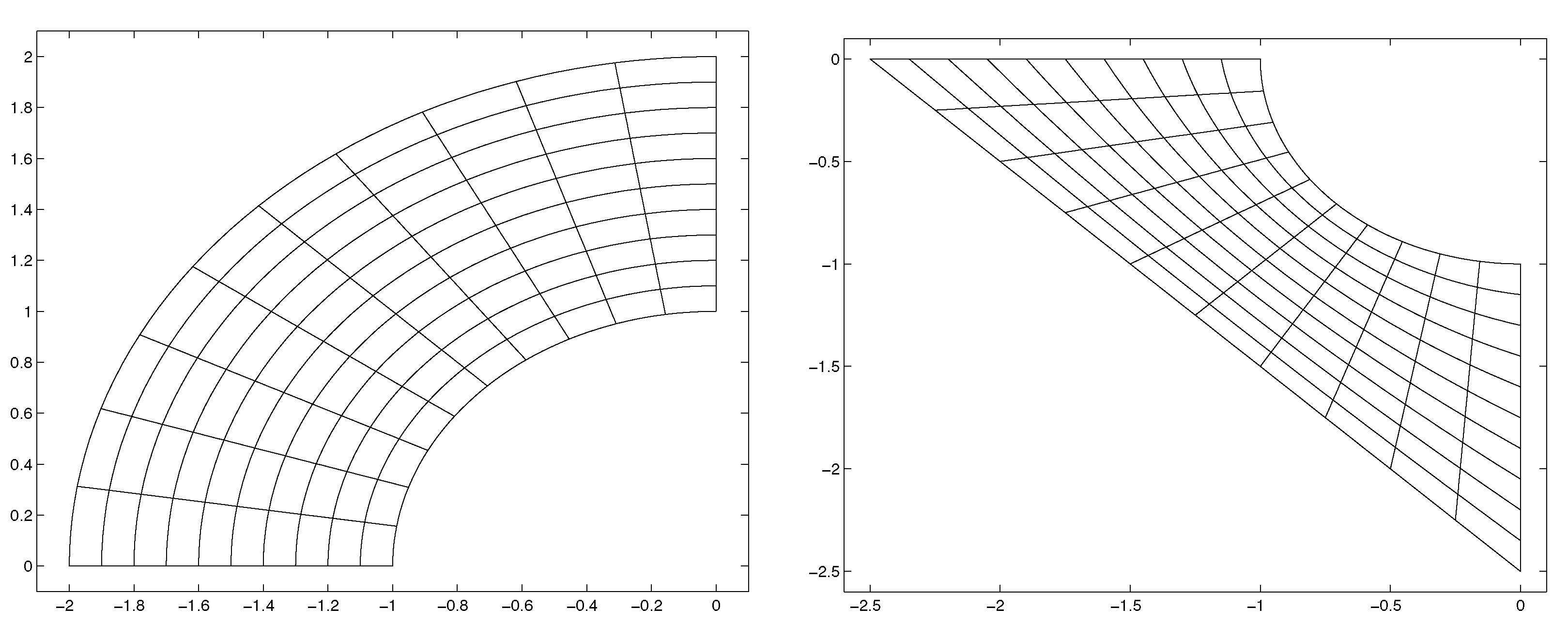
In Figure 3, we illustrate that for simple boundary curves, the Coons map is regular. Also, note that under the constraints specified for the boundary curves, a regular Coons map establishes a diffeomorphism [17]. However, when the boundaries become too wavy, like in Figure 4, we observe overlapping isolines indicating that the map is not invertible.

3. Geometric Analysis of the Regularity of a Coons Map

In this section, we analyze how properties of the boundary curves affect the regularity of a Coons map $\mathbf{x}$. To formulate a sufficient condition for regularity, we make use of the following definitions, which allows us to quantify the “waviness” of the boundary curves:

$$\rho :=max\left\{\right|F_1^{\prime }\left(t\right)|:t\in [0, 1]\}.$$

(13)

$$F:=max\{S^1, S^2\},\mathrm{where}$$

(14)

$$S^1:=\rho \underset{v\in [0,1]}{max}\parallel {\mathbf{S}}_1\left(v\right)\parallel ,S^2:=\rho \underset{u\in [0,1]}{max}\parallel {\mathbf{S}}_2\left(u\right)\parallel ,\mathrm{with}$$

(15)

$$\begin{array}{ccc}\hfill {\mathbf{S}}_1\left(v\right)& :=& \beta \left(v\right)-\delta \left(v\right)+[F_0\left(v\right)\delta \left(0\right)+F_1\left(v\right)\delta \left(1\right)]-[F_0\left(v\right)\beta \left(0\right)+F_1\left(v\right)\beta \left(1\right)]\hfill \\ \hfill {\mathbf{S}}_2\left(u\right)& :=& \gamma \left(u\right)-\alpha \left(u\right)+[F_0\left(u\right)\alpha \left(0\right)+F_1\left(u\right)\alpha \left(1\right)]-[F_0\left(u\right)\gamma \left(0\right)+F_1\left(u\right)\gamma \left(1\right)].\hfill \end{array}$$

Furthermore,

$$M:=max\left\{\underset{(u,v)\in {[0,1]}^2}{max}\parallel {\mathbf{C}}_1(u,v)\parallel ,\underset{(u,v)\in {[0,1]}^2}{max}\parallel {\mathbf{C}}_2(u, v)\parallel \right\}.$$

(16)

with

$$\begin{array}{ccc}\hfill {\mathbf{C}}_1(u, v)& :=& F_0\left(v\right){\alpha }^{\prime }\left(u\right)+F_1\left(v\right){\gamma }^{\prime }\left(u\right)\hfill \end{array}$$

(17)

$$\begin{array}{ccc}\hfill {\mathbf{C}}_2(u, v)& :=& F_0\left(u\right){\delta }^{\prime }\left(v\right)+F_1\left(u\right){\beta }^{\prime }\left(v\right).\hfill \end{array}$$

(18)

Theorem 1.

If there exists some $\tau >0$ such that

$$\det [{\mathbf{C}}_1(u, v),{\mathbf{C}}_2(u, v)]\ge \tau \forall (u, v)\in {[0, 1]}^2$$

(19)

and

$$2MF+F^2<\tau ,$$

(20)

then the Coons map $\mathbf{x}$ with respect to α, β, γ, δ is regular.

Proof of Theorem 1.

Computing the partial derivatives of the Coons map $\mathbf{x}$ according to (8) and using the definitions of ${\mathbf{S}}_1$, ${\mathbf{S}}_2$ according to (15) and ${\mathbf{C}}_1$, ${\mathbf{C}}_2$ according to (17), we obtain

$$\begin{array}{ccc}\hfill {\mathbf{x}}_u(u, v)& =& F_1^{\prime }\left(u\right){\mathbf{S}}_1\left(v\right)+{\mathbf{C}}_1(u, v),\hfill \end{array}$$

(21)

$$\begin{array}{ccc}\hfill {\mathbf{x}}_v(u, v)& =& F_1^{\prime }\left(v\right){\mathbf{S}}_2\left(u\right)+{\mathbf{C}}_2(u, v).\hfill \end{array}$$

(22)

By using (14), we obtain

$$|F_1^{\prime }\left(u\right)| · \parallel {\mathbf{S}}_1\left(v\right)\parallel \le F\mathrm{and}|F_1^{\prime }\left(v\right)| · \parallel {\mathbf{S}}_2\left(u\right)\parallel \le F.$$

(23)

Exploiting the linearity of the determinant with respect to both arguments, we obtain

$$\begin{array}{ccc}\hfill \det ({\mathbf{x}}_u, {\mathbf{x}}_v)& =& F_1^{\prime }\left(u\right)F_1^{\prime }\left(v\right)\det [{\mathbf{S}}_1\left(v\right), {\mathbf{S}}_2\left(u\right)]+F_1^{\prime }\left(u\right)\det [{\mathbf{S}}_1\left(v\right), {\mathbf{C}}_2(u, v)]+\hfill \\ & & F_1^{\prime }\left(v\right)\det [{\mathbf{C}}_1(u, v), {\mathbf{S}}_2\left(u\right)]+\det [{\mathbf{C}}_1(u, v), {\mathbf{C}}_2(u, v)].\hfill \\ & \ge & \det [{\mathbf{C}}_1(u, v),{\mathbf{C}}_2(u, v)]-\left\{\right|F_1^{\prime }\left(u\right)F_1^{\prime }\left(v\right)\det [{\mathbf{S}}_1\left(v\right), {\mathbf{S}}_2\left(u\right)]|+\hfill \\ & & |F_1^{\prime }\left(u\right)\det [{\mathbf{S}}_1\left(v\right), {\mathbf{C}}_2(u, v)]|+|F_1^{\prime }\left(v\right)\det [{\mathbf{C}}_1(u, v), {\mathbf{S}}_2\left(u\right)]\left|\right\}.\hfill \end{array}$$

By using (19), we obtain

$$\begin{array}{ccc}\hfill \det ({\mathbf{x}}_u, {\mathbf{x}}_v)& \ge & \tau -\left\{\right|F_1^{\prime }\left(u\right)F_1^{\prime }\left(v\right)| · \parallel {\mathbf{S}}_1\left(v\right)\parallel ·\parallel {\mathbf{S}}_2\left(u\right)\parallel +\hfill \\ & & |F_1^{\prime }\left(u\right)| · \parallel {\mathbf{S}}_1\left(v\right)\parallel · \parallel {\mathbf{C}}_2(u, v)\parallel +\hfill \\ & & |F_1^{\prime }\left(v\right)| · \parallel {\mathbf{C}}_1(u, v)\parallel · \parallel {\mathbf{S}}_2\left(u\right)\parallel \}.\hfill \end{array}$$

Due to (23), we obtain

$$\det ({\mathbf{x}}_u, {\mathbf{x}}_v)\ge \tau -(F^2+2FM).$$

Relation (20) finally ensures that $\det ({\mathbf{x}}_u, {\mathbf{x}}_v)>0$. That means the Jacobian is nowhere zero. The inverse function theorem ensures therefore that the Coons map locally is a diffeomorphism.    □

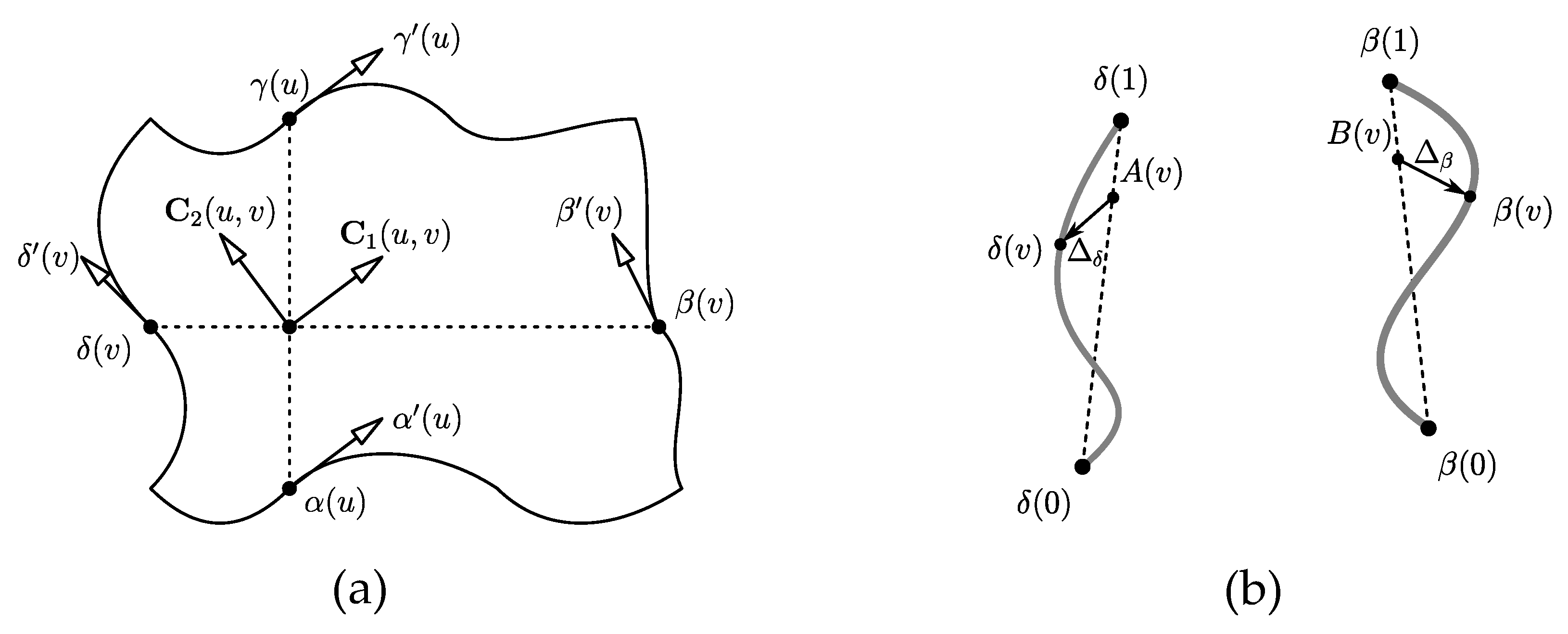
In the following, we give geometric interpretations of the terms used to formulate the above sufficient condition. The vectors ${\mathbf{C}}_1$ and ${\mathbf{C}}_2$ are defined as convex combinations of tangent vectors on opposite boundary curves and can be considered as approximations of the partial derivatives ${\mathbf{x}}_u$, ${\mathbf{x}}_v$ of $\mathbf{x}$. The lower bound (19) related to $\det ({\mathbf{C}}_1, {\mathbf{C}}_2)$ prevents the angle $\theta$ between the vectors ${\mathbf{C}}_1$ and ${\mathbf{C}}_2$ from approaching 0 or $\pi$. See Figure 5a.

The vectors $S_1$ and $S_2$ encode both the similarity and the “waviness” of opposite boundary curves as can be seen as follows (see Figure 5b). Let $A\left(v\right)$ and $B\left(v\right)$ denote line segments joining the end points of the boundary curves $\delta$ and $\beta$: $A\left(v\right):=F_0\left(v\right)\delta \left(0\right)+F_1\left(v\right)\delta \left(1\right)$ and $B\left(v\right):=F_0\left(v\right)\beta \left(0\right)+F_1\left(v\right)\beta \left(1\right)$. Now, let ${\mathrm{\Delta }}_{\delta }$ denote the deviation of $\delta$ from A and ${\mathrm{\Delta }}_{\beta }$ denote the deviation of $\beta$ from B: ${\mathrm{\Delta }}_{\delta }\left(v\right):=\delta \left(v\right)-A\left(v\right)$ and ${\mathrm{\Delta }}_{\beta }\left(v\right):=\beta \left(v\right)-B\left(v\right)$. Then, $S_1\left(v\right)$ is the difference in the deviations: $S_1\left(v\right)={\mathrm{\Delta }}_{\delta }\left(v\right)-{\mathrm{\Delta }}_{\beta }\left(v\right)$. From this reformulation, it is clear that $S_1\left(v\right)$ vanishes if $\delta$ and $\beta$ are line segments (because both deviations are zero) or if $\delta$ and $\beta$ are parallel translates (because the deviations are equal). The same applies to $S_2\left(v\right)$. These special cases will be handled in the following corollaries.

Corollary 1.

Suppose that $\gamma \left(t\right)=\alpha \left(t\right)+{\mathbf{w}}_1$ and $\beta \left(t\right)=\delta \left(t\right)+{\mathbf{w}}_2$ where ${\mathbf{W}}_1$ and ${\mathbf{W}}_2$ are constant vectors such that $\mathrm{Im}\left(\alpha \right)\cap \mathrm{Im}\left(\gamma \right)=\varnothing$ and $\mathrm{Im}\left(\delta \right)\cap \mathrm{Im}\left(\beta \right)=\varnothing$.

If there exists some $\tau >0$ such that

$$\det [{\alpha }^{\prime }\left(t_1\right), {\beta }^{\prime }\left(t_2\right)]\ge \tau \forall t_1, t_2\in [0, 1],$$

(24)

then the corresponding Coons map is regular.

Proof. 

In this special case, we obtain

$${\mathbf{C}}_1(u, v)=[F_0\left(v\right)+F_1\left(v\right)]{\alpha }^{\prime }\left(u\right)={\alpha }^{\prime }\left(u\right)$$

(25)

and similarly, ${\mathbf{C}}_2(u, v)={\beta }^{\prime }\left(v\right)$. Therefore, condition (19) reduces to (24). Since $\delta$ and $\beta$ are parallel translates $S_1\left(v\right)={\mathrm{\Delta }}_{\delta }\left(v\right)-{\mathrm{\Delta }}_{\delta }\left(v\right)=0$. Since $\alpha$ and $\gamma$ are also parallel, we obtain $S_2\left(v\right)=0$. As a result, the value of F from definition (14) is zero and (20) is trivially fulfilled.    □

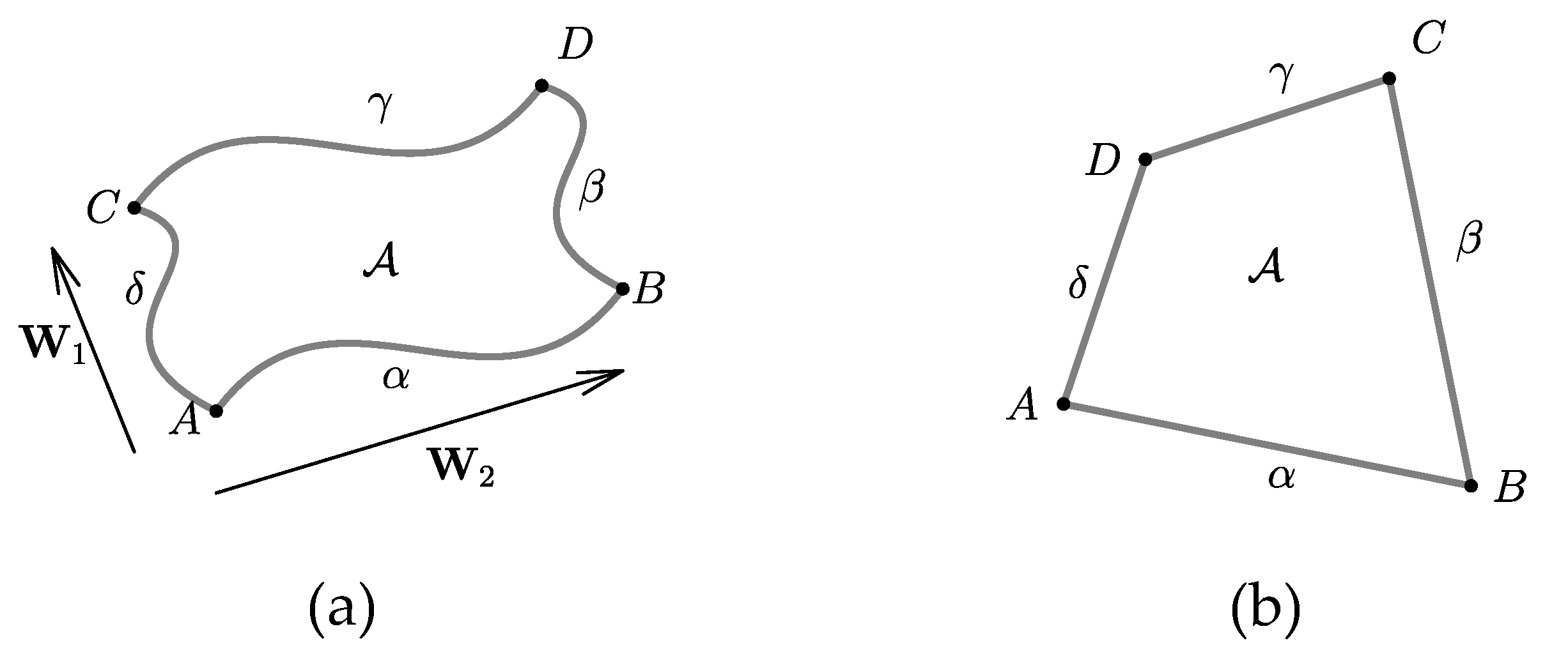
The following simple case allows to apply Coons maps to four-sided tesselations of complex domains.

Corollary 2.

Suppose that the images of the curves α, β, γ, δ form a convex quadrilateral. Assume that the boundary curves are linearly parameterized. Then, the corresponding Coons map with the linear blending function  $F_1\left(t\right)=t$ is regular.

Proof. 

Let us denote the four corners of the quadrilateral by A, B, C, D as shown in Figure 6b. Therefore, the expressions of ${\mathbf{S}}_1\left(v\right)$ and ${\mathbf{S}}_2\left(u\right)$ become:

$$\begin{array}{ccc}\hfill {\mathbf{S}}_1\left(v\right)& =& \beta \left(v\right)-\delta \left(v\right)+\left[\right(1-v)A+vD]-\left[\right(1-v)B+vC],\hfill \end{array}$$

(26)

$$\begin{array}{ccc}\hfill {\mathbf{S}}_2\left(u\right)& =& \gamma \left(u\right)-\alpha \left(u\right)+\left[\right(1-u)A+uB]-\left[\right(1-u)D+uC].\hfill \end{array}$$

(27)

Since we have the following convex combination parametrizations

$$\begin{array}{ccc}\hfill \alpha \left(u\right)=(1-u)A+uB,& & \gamma \left(u\right)=(1-u)D+uC,\hfill \end{array}$$

(28)

$$\begin{array}{ccc}\hfill \beta \left(v\right)=(1-v)B+vC,& & \delta \left(v\right)=(1-v)A+vD,\hfill \end{array}$$

(29)

we deduce

$${\mathbf{S}}_1\left(v\right)={\mathbf{S}}_2\left(u\right)=0\forall u,v\in [0,1].$$

(30)

As a result, the value of F from definition (14) is zero and (20) is trivially fulfilled. On the other hand, the tangents are constantly given by

$$\begin{array}{ccc}\hfill {\alpha }^{\prime }\left(u\right)=\overrightarrow{AB},& & {\gamma }^{\prime }\left(u\right)=\overrightarrow{DC},\hfill \end{array}$$

(31)

$$\begin{array}{ccc}\hfill {\beta }^{\prime }\left(v\right)=\overrightarrow{BC},& & {\delta }^{\prime }\left(v\right)=\overrightarrow{AD}.\hfill \end{array}$$

(32)

As a consequence, the left hand side of (19) becomes

$$\begin{array}{ccc}\hfill det(C1, C2)& =& vudet(\overrightarrow{DC}, \overrightarrow{BC})+(1-v)udet(\overrightarrow{AB}, \overrightarrow{BC})+\hfill \\ & & v(1-u)det(\overrightarrow{DC}, \overrightarrow{AD})+(1-v)(1-u)det(\overrightarrow{AB}, \overrightarrow{AD}).\hfill \end{array}$$

The convexity of the quadrilateral $[A, B, C, D]$ ensures that

$$\begin{array}{ccc}\hfill det(\overrightarrow{AB}, \overrightarrow{AD})>0,& & det(\overrightarrow{AB}, \overrightarrow{BC})>0,\hfill \end{array}$$

(33)

$$\begin{array}{ccc}\hfill det(\overrightarrow{DC}, \overrightarrow{AD})>0,& & det(\overrightarrow{DC}, \overrightarrow{BC})>0.\hfill \end{array}$$

(34)

Thus, (19) holds with $\tau$ being the minimum of the above four positive determinants.    □

4. Sufficient Conditions for Polynomial Coons Maps

From now on, we suppose that the boundary curves $\alpha$, $\beta$, $\gamma$, $\delta$ are Bézier curves of degree n with control points ${\alpha }_i$, ${\beta }_i$, ${\gamma }_i$, ${\delta }_i$ $(i=0,\cdots , n)$, respectively:

$$\alpha \left(t\right)=\sum _{i=0}^n{\alpha }_i{B}_i^n\left(t\right),\beta \left(t\right)=\sum _{i=0}^n{\beta }_i{B}_i^n\left(t\right),$$

(35)

$$\gamma \left(t\right)=\sum _{i=0}^n{\gamma }_i{B}_i^n\left(t\right),\delta \left(t\right)=\sum _{i=0}^n{\delta }_i{B}_i^n\left(t\right).$$

(36)

The polynomial blending function $F_1$ is also expressed in Bézier form:

$$F_1\left(t\right)=\sum _{i=0}^n{\varphi }_i{B}_i^n\left(t\right)=1-F_0\left(t\right).$$

(37)

From Theorem 1, we will now derive conditions for the Bézier points of the boundary curves and blending functions that guarantee the regularity of the Coons map. For this, we introduce

$$\tilde{F}:=max\{{\tilde{S}}^1, {\tilde{S}}^2\},\mathrm{where}$$

(38)

$$\begin{array}{ccc}\hfill {\tilde{S}}^1& :=& \underset{i=0,\cdots ,n}{max}\{\rho \parallel ({\beta }_i-{\delta }_i)+{\varphi }_i({\gamma }_0-{\gamma }_n+{\alpha }_n-{\alpha }_0)+({\alpha }_0-{\alpha }_n)\parallel \}\hfill \\ \hfill {\tilde{S}}^2& :=& \underset{i=0,\cdots ,n}{max}\{\rho \parallel ({\gamma }_i-{\alpha }_i)+{\varphi }_i({\gamma }_0-{\gamma }_n+{\alpha }_n-{\alpha }_0)+({\alpha }_0-{\gamma }_0)\parallel \}.\hfill \end{array}$$

Furthermore, we define

$$\begin{array}{c}{A}_{ij}:=n^{2}det[{\alpha }_{i+1}-{\alpha }_i,{\delta }_{j+1}-{\delta }_j],B_{ij}:=n^{2}det[{\alpha }_{i+1}-{\alpha }_i,{\beta }_{j+1}-{\beta }_j],\hfill \\ C_{ij}:=n^{2}det[{\gamma }_{i+1}-{\gamma }_i,{\delta }_{j+1}-{\delta }_j],D_{ij}:=n^{2}det[{\gamma }_{i+1}-{\gamma }_i,{\beta }_{j+1}-{\beta }_j],\hfill \end{array}$$

and

$$\tilde{\tau }:=\underset{i,j}{min}\{A_{ij}, B_{ij}, C_{ij}, D_{ij}\}.$$

(39)

Theorem 2.

Let $\tilde{M}$ be a constant such that

$$\begin{array}{ccc}\hfill n\parallel {\varphi }_j({\gamma }_{i+1}-{\gamma }_i+{\alpha }_i-{\alpha }_{i+1})+({\alpha }_{i+1}-{\alpha }_i)\parallel & \le & \tilde{M}\hfill \\ \hfill n\parallel {\varphi }_j({\beta }_{i+1}-{\beta }_i+{\delta }_i-{\delta }_{i+1})+({\delta }_{i+1}-{\delta }_i)\parallel & \le & \tilde{M},\hfill \end{array}$$

(40)

for all $i=0,\cdots , n-1$ and $j=0,\cdots , n$.

Suppose that $A_{ij}$, $B_{ij}$, $C_{ij}$, $D_{ij}$ are all positive for all  $i, j=0,\cdots , n-1$. Then,

$$2\tilde{M}\tilde{F}+{\tilde{F}}^2<\tilde{\tau }$$

(41)

is sufficient for $\mathbf{x}$ to be regular.

Proof of Theorem 2.

According to the Bézier expression of $\alpha$, $\beta$, $\gamma$, $\delta$, we can formulate ${\mathbf{S}}_1$ and ${\mathbf{S}}_2$ in terms of the control points:

$$\begin{array}{ccc}\hfill {\mathbf{S}}_1\left(v\right)& =& \sum _{i=0}^n({\beta }_i-{\delta }_i)B_i^n\left(v\right)+F_1\left(v\right)({\gamma }_0-{\gamma }_n+{\alpha }_n-{\alpha }_0)+({\alpha }_0-{\alpha }_n),\hfill \\ \hfill {\mathbf{S}}_2\left(u\right)& =& \sum _{i=0}^n({\gamma }_i-{\alpha }_i)B_i^n\left(u\right)+F_1\left(u\right)({\alpha }_n-{\gamma }_n+{\gamma }_0-{\alpha }_0)+({\alpha }_0-{\gamma }_0).\hfill \end{array}$$

After a few rearrangements in which we use (37), we obtain:

$$\begin{array}{ccc}\hfill {\mathbf{S}}_1\left(v\right)& =& \sum _{i=0}^n[({\beta }_i-{\delta }_i)+{\varphi }_i({\gamma }_0-{\gamma }_n+{\alpha }_n-{\alpha }_0)+({\alpha }_0-{\alpha }_n)]B_i^n\left(v\right),\hfill \\ \hfill {\mathbf{S}}_2\left(u\right)& =& \sum _{i=0}^n[({\gamma }_i-{\alpha }_i)+{\varphi }_i({\alpha }_n-{\gamma }_n+{\gamma }_0-{\alpha }_0)+({\alpha }_0-{\gamma }_0)]B_i^n\left(u\right).\hfill \end{array}$$

By using the Bézier representation, the function ${\mathbf{C}}_1$ can be expressed as

$$\begin{array}{ccc}\hfill {\mathbf{C}}_1(u, v)& =& (1-F_1\left(v\right))\sum _{i=0}^{n-1}[{\alpha }_{i+1}-{\alpha }_i]B_i^{n-1}\left(u\right)+F_1\left(v\right)\sum _{i=0}^{n-1}[{\gamma }_{i+1}-{\gamma }_i]B_i^{n-1}\left(u\right)\hfill \\ & =& \sum _{i=0}^{n-1}\sum _{j=0}^n[({\alpha }_{i+1}-{\alpha }_i)+{\varphi }_j({\gamma }_{i+1}-{\gamma }_i-{\alpha }_{i+1}+{\alpha }_i)]B_i^{n-1}\left(u\right)B_j^n\left(v\right).\hfill \end{array}$$

Additionally, the expression of ${\mathbf{C}}_2$ can be formulated in a similar way. Thus, relation (40) implies the following bounds

$$\parallel {\mathbf{C}}_1(u, v)\parallel \le \tilde{M},\parallel {\mathbf{C}}_2(u, v)\parallel \le \tilde{M}\forall (u, v)\in {[0, 1]}^2.$$

According to the multilinearity of the determinant, we have

$$\begin{array}{ccc}\hfill det[{\mathbf{C}}_1, {\mathbf{C}}_2]& =& F_0\left(v\right)F_0\left(u\right)det[{\alpha }^{\prime }\left(u\right), {\delta }^{\prime }\left(v\right)]+F_0\left(v\right)F_1\left(u\right)det[{\alpha }^{\prime }\left(u\right), {\beta }^{\prime }\left(v\right)]+\hfill \\ & & F_1\left(v\right)F_0\left(u\right)det[{\gamma }^{\prime }\left(u\right), {\delta }^{\prime }\left(v\right)]+F_1\left(v\right)F_1\left(u\right)det[{\gamma }^{\prime }\left(u\right), {\beta }^{\prime }\left(v\right)].\hfill \end{array}$$

On account of the fact that

$${\alpha }^{\prime }\left(u\right)=\sum _{i=0}^{n-1}n({\alpha }_{i+1}-{\alpha }_i)B_i^{n-1}\left(u\right)$$

(42)

and similar relations for $\beta$, $\gamma$, $\delta$, we deduce from (39) that

$$det[{\mathbf{C}}_1(u,v),{\mathbf{C}}_2(u,v)]\ge \sum _{i=0}^{n-1}\sum _{j=0}^{n-1}\tilde{\tau }{B}_i^{n-1}\left(u\right)B_j^{n-1}\left(v\right)=\tilde{\tau }.$$

(43)

The inequality

$$det[{\mathbf{x}}_u,{\mathbf{x}}_v]\ge det[{\mathbf{C}}_1(u,v),{\mathbf{C}}_2(u,v)]-({\tilde{F}}^2+2\tilde{F}\tilde{M})$$

(44)

concludes the proof.    □

We consider a parametrized example to illustrate the geometric meaning of the criterion (41). Suppose that the boundary curves $\alpha$, $\beta$, $\gamma$, $\delta$ are Bézier curves of degree 2 with end points ${\alpha }_0={\delta }_0$, ${\alpha }_2={\beta }_0$, ${\gamma }_0={\delta }_2$, ${\gamma }_2={\beta }_2$ lying on the corners of a square of edge length l and ${\alpha }_1=(l/2, \epsilon )$, ${\gamma }_1=(l/2, l-\epsilon )$, ${\delta }_1=(\epsilon , l/2)$, and ${\beta }_1=(l-\epsilon , l/2)$ with $\epsilon >0$. Figure 7a illustrates the situation.

To simplify the notation, we introduce the following vectors for the edges of the Bézier polygons of the four boundary curves:

$${\overrightarrow{\alpha }}_{i+1}={\alpha }_{i+1}-{\alpha }_i,{\overrightarrow{\beta }}_{i+1}={\beta }_{i+1}-{\beta }_i,{\overrightarrow{\gamma }}_{i+1}={\gamma }_{i+1}-{\gamma }_i,{\overrightarrow{\delta }}_{i+1}={\delta }_{i+1}-{\delta }_i,i=0, 1.$$

In this situation, we obtain for the determinants $A_{ij}$:

$$\begin{array}{ccc}\hfill A_{00}& =& 4det({\overrightarrow{\alpha }}_1,{\overrightarrow{\delta }}_1)=4\left|\begin{array}{cc}{\displaystyle \frac{\ell }{2}}& \epsilon \\ \epsilon & {\displaystyle \frac{\ell }{2}}\end{array}\right|=4({\displaystyle \frac{{\ell }^2}{4}}-{\epsilon }^2)={\ell }^2-4{\epsilon }^2\hfill \\ \hfill A_{10}& =& 4det({\overrightarrow{\alpha }}_2,{\overrightarrow{\delta }}_1)=4\left|\begin{array}{cc}{\displaystyle \frac{\ell }{2}}& \epsilon \\ -\epsilon & {\displaystyle \frac{\ell }{2}}\end{array}\right|={\ell }^2+4{\epsilon }^2\hfill \\ \hfill A_{01}& =& 4det({\overrightarrow{\alpha }}_1,{\overrightarrow{\delta }}_2)=4\left|\begin{array}{cc}{\displaystyle \frac{\ell }{2}}& -\epsilon \\ \epsilon & {\displaystyle \frac{\ell }{2}}\end{array}\right|={\ell }^2+4{\epsilon }^2\hfill \\ \hfill A_{11}& =& 4det({\overrightarrow{\alpha }}_2,{\overrightarrow{\delta }}_2)=4\left|\begin{array}{cc}{\displaystyle \frac{\ell }{2}}& -\epsilon \\ -\epsilon & {\displaystyle \frac{\ell }{2}}\end{array}\right|={\ell }^2-4{\epsilon }^2\hfill \end{array}$$

For reasons of symmetry, the determinants $B_{ij}$, $C_{ij}$, $D_{ij}$ provide the same expressions. Thus, we obtain for the minimum $\tilde{\tau }$ of these determinants $\tilde{\tau }={\ell }^2-4{\epsilon }^2$. $\tilde{\tau }$ is the right side of the inequality (41) and corresponds to the smallest parallelogram spanned by two vectors of the four Bézier polygons.

Now, we will consider the terms on the left side of the sufficiency criterion (41). To compute $\tilde{F}$ according to (38), we first note that $({\gamma }_0-{\gamma }_2)+({\alpha }_2-{\alpha }_0)=0$, because the points correspond to the corners of a square. Consequently, we obtain for ${\tilde{S}}^1$:

$${\tilde{S}}^1=\rho ·max\left\{\parallel ({\beta }_0-{\delta }_0)+({\alpha }_0-{\alpha }_2)\parallel ,\parallel ({\beta }_1-{\delta }_1)+({\alpha }_0-{\alpha }_2)\parallel ,\parallel ({\beta }_2-{\delta }_2)+({\alpha }_0-{\alpha }_2)\parallel \right\}.$$

In our geometric situation, this simplifies to

$${\tilde{S}}^1=\rho max\left\{0, \parallel (l-2\epsilon )·{\overrightarrow{e}}_1-l·{\overrightarrow{e}}_1\parallel , 0\right\}=2\rho \epsilon$$

with ${\overrightarrow{e}}_1=(1, 0)$. In a similar way, we obtain ${\tilde{S}}^2=2\rho \epsilon$, which means $\tilde{F}=2\rho \epsilon$.

In our example, we use linear blending functions, which yields $\rho =1$ as the maximum value of $|F_1^{\prime }\left(t\right)|$. As already mentioned in Section 3, $\tilde{F}$ relates to the deviation in waviness of opposite boundary curves, which in this example is bounded by $2\epsilon$.

$\tilde{M}$ is an upper bound for $\parallel {\mathbf{C}}_1(u, v)\parallel$ and $\parallel {\mathbf{C}}_2(u, v)\parallel$ with ${\mathbf{C}}_1(u, v)$, ${\mathbf{C}}_2(u, v)$ representing approximations of the partial derivatives of the Coons map with respect to u and v. $\tilde{M}$ is computed from (40), which involves the vectors

$${\varphi }_j({\overrightarrow{\gamma }}_i-{\overrightarrow{\alpha }}_i)+{\overrightarrow{\alpha }}_i\mathrm{with}i=1, 2\mathrm{and}j=0, 1, 2.$$

Here, ${\varphi }_0=0$, ${\varphi }_1=1/2$, and ${\varphi }_2=1$ are the coefficients of $F_1\left(t\right)=t$ degree elevated to a quadratic Bézier representation:

$$F_1\left(t\right)=0B_0^1\left(t\right)+1B_1^1\left(t\right)=0B_0^2+{\displaystyle \frac{1}{2}}{B}_1^2\left(t\right)+1B_2^2\left(t\right).$$

Thus, we obtain

$$\begin{array}{ccc}\hfill \mathrm{for}j=0& :& {\overrightarrow{\alpha }}_1,{\overrightarrow{\alpha }}_2,\hfill \\ \hfill \mathrm{for}j=1& :& {\displaystyle \frac{1}{2}}({\overrightarrow{\gamma }}_1+{\overrightarrow{\alpha }}_1),{\displaystyle \frac{1}{2}}({\overrightarrow{\gamma }}_2+{\overrightarrow{\alpha }}_2),\mathrm{and}\hfill \\ \hfill \mathrm{for}j=2& :& {\overrightarrow{\gamma }}_1,{\overrightarrow{\gamma }}_2.\hfill \end{array}$$

According to (40), $\tilde{M}$ must be equal to or larger than twice the length of the longest of these vectors. This gives

$$\tilde{M}=2·\sqrt{{\displaystyle \frac{l^2}{4}}+{\epsilon }^2}.$$

Therefore, for our example, the sufficiency criterion $2\tilde{M}\tilde{F}+{\tilde{F}}^2<\tilde{\tau }$ takes the form

$$8\epsilon \sqrt{{\displaystyle \frac{l^2}{4}}+{\epsilon }^2}<l^2-8{\epsilon }^2.$$

Using the relation $l^2=\lambda {\epsilon }^2$, we obtain the inequality

$$8\sqrt{{\displaystyle \frac{\lambda }{4}}+1}<\lambda -8.$$

(45)

Solving (45) for $\lambda$, we obtain $\lambda >32$, i.e.,

$$\epsilon <0.176l.$$

This example shows the strengths and weaknesses of the regularity criterion (41). On the one hand, the method allows us to calculate analytically parameter ranges for which the regularity of the mapping is ensured. On the other hand, our experiments showed that the criterion is sometimes much stricter than necessary. Figure 7b shows the Coons map for $\epsilon =0.175$. However, visual inspection indicates that the considered Coons map is regular for much larger values of $\epsilon$. Therefore, we searched for less restrictive sufficient conditions for the regularity of a Coons map. As a starting point, we rewrite a polynomial Coons map as a bivariate Bézier map.

Lemma 1.

Suppose the boundary curves  α, β, γ, δ and the blending function are given according to (35)–(37). Then, the Coons map is a bivariate polynomial that can be written in Bézier form

$$\mathbf{x}(u, v)=\sum _{i=0}^n\sum _{j=0}^n{\mathbf{E}}_{ij}{B}_i^n\left(u\right)B_j^n\left(v\right)$$

(46)

with control points

$$\begin{array}{ccc}\hfill {\mathbf{E}}_{ij}& :=& {\delta }_j-{\alpha }_0+{\alpha }_i+{\varphi }_j({\gamma }_i-{\alpha }_i+{\alpha }_0-{\gamma }_0)\hfill \\ \hfill & & {\varphi }_i[{\alpha }_0-{\alpha }_n+{\beta }_j-{\delta }_j+{\varphi }_j({\alpha }_n-{\gamma }_n+{\gamma }_0-{\alpha }_0)].\hfill \end{array}$$

(47)

Proof. 

Obvious. See also [18] for a similar discussion.    □

Theorem 3.

A polynomial Coons map $\mathbf{x}$$:{[0, 1]}^2⟶{\mathbf{R}}^2$ of degree $(n, n)$ with Bézier points ${\mathbf{E}}_{ij}$ according to (47) is regular, if for all $p, q=0,\cdots , 2n$

$$J_{pq}:=\sum _{{\displaystyle \genfrac{}{}{0pt}{}{i+k=p}{j+l=q}}}C(i, j, k, l){\displaystyle \frac{\left(\genfrac{}{}{0pt}{}{n}{i}\right)\left(\genfrac{}{}{0pt}{}{n}{k}\right)}{\left(\genfrac{}{}{0pt}{}{2n}{i+k}\right)}}{\displaystyle \frac{\left(\genfrac{}{}{0pt}{}{n}{j}\right)\left(\genfrac{}{}{0pt}{}{n}{l}\right)}{\left(\genfrac{}{}{0pt}{}{2n}{j+l}\right)}}>0$$

(48)

where

$$\begin{array}{ccc}\hfill C(i, j , k ,l)& :=& {\displaystyle \frac{l}{n}}\left[{\displaystyle \frac{i}{n}}D(i-1, j, k, l-1)+(1-{\displaystyle \frac{i}{n}})D(i, j, k, l-1)\right]+\hfill \\ \hfill & & (1-{\displaystyle \frac{l}{n}})\left[{\displaystyle \frac{i}{n}}D(i-1, j, k, l)+(1-{\displaystyle \frac{i}{n}})D(i, j, k, l)\right]\hfill \end{array}$$

(49)

and

$$D(i, j, k, l):=n^2\det [{\mathbf{E}}_{i+1,j}-{\mathbf{E}}_{ij},{\mathbf{E}}_{k,l+1}-{\mathbf{E}}_{kl}].$$

(50)

Proof of Theorem 3.

The partial derivatives of the Bézier representation of $\mathbf{x}$ are

$$\begin{array}{ccc}\hfill {\mathbf{x}}_u(u, v)& =& \sum _{i=0}^{n-1}\sum _{j=0}^{n}n({\mathbf{E}}_{i+1, j}-{\mathbf{E}}_{ij})B_i^{n-1}\left(u\right)B_j^n\left(v\right),\hfill \end{array}$$

(51)

$$\begin{array}{ccc}\hfill {\mathbf{x}}_v(u, v)& =& \sum _{k=0}^n\sum _{l=0}^{n-1}n({\mathbf{E}}_{k, l+1}-{\mathbf{E}}_{kl})B_k^n\left(u\right)B_l^{n-1}\left(v\right).\hfill \end{array}$$

(52)

Consequently, the determinant can be expressed as follows

$$\det ({\mathbf{x}}_u, {\mathbf{x}}_v)=\sum _{i=0}^{n-1}\sum _{j=0}^n\sum _{k=0}^n\sum _{l=0}^{n-1}D(i, j, k, l)B_i^{n-1}\left(u\right)B_j^n\left(v\right)B_k^n\left(u\right)B_l^{n-1}\left(v\right).$$

(53)

After application of degree elevation with respect to the indices i and l, we obtain

$$\det ({\mathbf{x}}_u, {\mathbf{x}}_v)=\sum _{i=0}^n\sum _{j=0}^n\sum _{k=0}^n\sum _{l=0}^{n}C(i, j, k, l)B_i^n\left(u\right)B_j^n\left(v\right)B_k^n\left(u\right)B_l^n\left(v\right).$$

(54)

By using the product formula

$$B_i^n\left(t\right)B_k^n\left(t\right)={\displaystyle \frac{\left(\genfrac{}{}{0pt}{}{n}{i}\right)\left(\genfrac{}{}{0pt}{}{n}{k}\right)}{\left(\genfrac{}{}{0pt}{}{2n}{i+k}\right)}}{B}_{i+k}^{2n}\left(t\right)$$

(55)

the Jacobian can be written as

$$J(u, v):=\det ({\mathbf{x}}_u, {\mathbf{x}}_v)=\sum _{p=0}^{2n}\sum _{q=0}^{2n}{J}_{pq}{B}_p^{2n}\left(u\right)B_q^{2n}\left(v\right).$$

(56)

Since all coefficients $J_{pq}$ are positive, the Coons map $\mathbf{x}$ is regular.    □

Our experiments showed that the conditions of Theorem 3 are less restrictive than those of Theorem 2. The example illustrated in Figure 7 is an extreme case as the new conditions provide the regularity of the map for all $\epsilon <0.49$ (see Figure 8).

Figure 9 shows a different example with quartic boundary curves and shape parameter $\sigma$. Here, our experiments with both criteria provided results that are not too far apart. While the criterion of Theorem 2 is fulfilled for $\sigma <0.252$, the new criterion provides the regularity of the map for all $\sigma <0.324$. What remains is to answer the question of how far the larger value is away from the smallest $\sigma$ for which the map is not regular, i.e., the quest for tight necessary and sufficient conditions for regularity. This is addressed in the next section.

5. An Algorithm to Decide on the Regularity of a Coons Map

In this section, we formulate a condition for the regularity of a polynomial Coons map that is both necessary and sufficient. This criterion is based on a subdivision principle that also serves as the backbone of our decision algorithm.

We use the following notation to define the subdivision process. A Bézier map F defined on $[a, b]\times [c, d]$ can be subdivided into four Bézier submaps A, B, C, D each of which is defined on a corresponding subset:

$$\begin{array}{ccc}\hfill I^A:=[a, 0.5(a+b)]& \times & [c, 0.5(c+d\left)\right]\hfill \end{array}$$

(57)

$$\begin{array}{ccc}\hfill I^B:=[a, 0.5(a+b)]& \times & \left[0.5\right(c+d), d]\hfill \end{array}$$

(58)

$$\begin{array}{ccc}\hfill I^C:=[0.5(a+b), b]& \times & [c, 0.5(c+d\left)\right]\hfill \end{array}$$

(59)

$$\begin{array}{ccc}\hfill I^D:=[0.5(a+b), b]& \times & \left[0.5\right(c+d), d].\hfill \end{array}$$

(60)

Let $F_{pq}$ denote the control points of F. The four submaps are obtained in the following steps. First, we apply deCastelau’s algorithm with $u=1/2$ to the rows of the Bézier net:

$$\begin{array}{ccc}\hfill F_{pq}^{\left[0\right]}& :=& F_{pq}p, q=0,\cdots , n\mathrm{and}\hfill \end{array}$$

(61)

$$\begin{array}{ccc}\hfill F_{pq}^{\left[k\right]}& :=& 0.5(F_{p, q}^{[k-1]}+F_{p+1, q}^{[k-1]})\mathrm{for} p=0,\cdots , n-k\mathrm{and}k=1,\cdots , n.\hfill \end{array}$$

(62)

Then, we subdivide F at $u=1/2$ in two maps P, Q with Bézier coefficients

$$P_{pq}^{\left[0\right]}:=F_{0q}^{\left[p\right]},Q_{pq}^{\left[0\right]}:=F_{pq}^{[n-i]}\mathrm{for}p, q=0,\cdots , n$$

and apply deCastelau’s algorithm with $v=1/2$ to the columns of the Bézier nets of P and Q, i.e., for $q=0,\cdots , n-kandk=1,\cdots , n$    , we compute

$$\begin{array}{ccc}\hfill P_{pq}^{\left[k\right]}& :=& 0.5(P_{p,q}^{[k-1]}+P_{p,q+1}^{[k-1]})\hfill \end{array}$$

(63)

$$\begin{array}{ccc}\hfill Q_{pq}^{\left[k\right]}& :=& 0.5(Q_{p, q}^{[k-1]}+Q_{p, q+1}^{[k-1]}).\hfill \end{array}$$

(64)

Then, the control points of A, B, C and D are as follows $A_{pq}:=P_{p0}^{\left[q\right]}$, $B_{pq}:=P_{pq}^{[n-q]}$, $C_{pq}:=Q_{p0}^{\left[q\right]}$, $D_{pq}:=Q_{pq}^{[n-q]}$ for $p, q=0,\cdots , n$.

Theorem 4.

Let $\mathbf{x}$$:{[0,1]}^2⟶{\mathbf{R}}^2$ be a polynomial Coons map of degree $(n, n)$. Assume that $\mathbf{x}$ has been subdivided into ${\sigma }^2=4^k$ submaps ${\mathbf{x}}^{ij}$ defined on

$$I^{ij}:=[(i-1)/\sigma , i/\sigma ]\times [(j-1)/\sigma , j/\sigma ]i, j=1,\cdots , \sigma .$$

Let $J^{ij}$ denote the Jacobian of ${\mathbf{x}}^{ij}$ with Bézier coefficients $J_{pq}^{ij}$, $p, q=0, \cdots , 2n$ according to (56).

(i) 

If there is $\sigma \in \mathbb{N}$, such that all coefficients $J_{pq}^{ij}$$p, q=0,\cdots , 2n$ have the same sign, $\mathbf{x}$ is regular.

(ii) 

If $\mathbf{x}$ is regular, then there is $\sigma \in \mathbb{N}$ such that all coefficients $J_{pq}^{ij}$ have the same sign.

Proof 

(i) According to Theorem 3, each ${\mathbf{x}}^{ij}$ is regular. Since each submap ${\mathbf{x}}^{ij}$ is a restriction of the original map:

$${\mathbf{x}}^{ij}(u, v)=\mathbf{x}(u, v)\mathrm{if}(u, v)\in I^{ij},$$

$\mathbf{x}$ is regular on each $I^{ij}$. Since the union of the intervals $I^{ij}i, j=1,\cdots , \sigma$ is ${[0, 1]}^2$, $\mathbf{x}$ is regular.

(ii) Since $\mathbf{x}$ is regular, its Jacobian $J(u, v)$ is of constant sign for all $(u, v)\in {[0, 1]}^2$. Without loss of generality, we suppose that the sign of J is positive. Since the function J is continuous on the compact parameter space ${[0, 1]}^2$, there must exist some $\rho >0$ such that

$$J(u, v)\ge \rho \forall (u, v)\in [0, 1]\times [0, 1].$$

(65)

To simplify notation, we fix $(i, j)$ and denote the domain of $I^{ij}$ by $[a, b]\times [c, d]$. Let

$$P^{ij}(u_1,\cdots , u_{2n};v_1,\cdots , v_{2n})$$

be the blossom [19] of the polynomial $J^{ij}$:

$$J^{ij}(u, v)=P^{ij}(u,..\left[2n\right]..,u; v,..\left[2n\right]..,v)$$

(66)

where we use the notation $s,..\left[m\right].., s$ for an m times repetition of s.

Define $h:=1/\left(2n\sigma \right)$ and $a_p:=a+ph$, $c_q:=c+qh$ for $p=0,\cdots , 2n$ and $q=0,\cdots , 2n$. Now, we apply the multivariate Taylor expansion of the first order to the blossom $P^{ij}$ at $(a_p,..\left[2n\right].., a_p; c_q,..\left[2n\right].., c_q)$.

$$\begin{array}{ccc}& & P^{ij}(a,..[2n-p].., a, b,..\left[p\right].., b; c,..[2n-q].., c, d,..\left[q\right].., d)=\hfill \\ & & P^{ij}(a_p,..\left[2n\right].., a_p; c_q,..\left[2n\right].., c_q)+\hfill \\ & & \sum _{r=1}^{2n-p}(a-a_p){\displaystyle \frac{\partial }{\partial u_r}}{P}^{ij}(a_p,..\left[2n\right].., a_p; c_q,..\left[2n\right].., c_q)+\hfill \\ & & \sum _{r=2n-p+1}^{2n}(b-a_p){\displaystyle \frac{\partial }{\partial u_r}}{P}^{ij}(a_p,..\left[2n\right].., a_p; c_q,..\left[2n\right].., c_q)+\hfill \\ & & \sum _{r=1}^{2n-q}(c-c_q){\displaystyle \frac{\partial }{\partial v_r}}{P}^{ij}(a_p,..\left[2n\right]..,a_p; c_q,..\left[2n\right].., c_q)+\hfill \\ & & \sum _{r=2n-q+1}^{2n}(d-c_q){\displaystyle \frac{\partial }{\partial v_r}}{P}^{ij}(a_p,..\left[2n\right].., a_p; c_q,..\left[2n\right].., c_q)+\mathcal{O}\left(h^2\right).\hfill \end{array}$$

Due to the symmetry [19] of the blossom function, we obtain

$$\begin{array}{c}{P}^{ij}(a,..[2n-p].., a, b,..\left[p\right].., b; c,..[2n-q].., c, d,..\left[q\right]..d)=\hfill \\ P^{ij}(a_p,..\left[2n\right].., a_p; c_q,..\left[2n\right].., c_q)+\mathcal{O}\left(h^2\right).\hfill \end{array}$$

(67)

Thus, we obtain the following for control points of J:

$$J_{pq}^{ij}=J^{ij}(a_p,c_q)+\mathcal{O}\left(h^2\right).$$

(68)

Combining (65) and (68), there must exist some constant $C>0$ such that

$$\begin{array}{ccc}\hfill J_{pq}^{ij}& =& J^{ij}(a_p,c_q)+J_{pq}^{ij}-J^{ij}(a_p,c_q)\hfill \end{array}$$

(69)

$$\begin{array}{ccc}& \ge & J(a_p,c_q)-C{h}^2\hfill \end{array}$$

(70)

$$\begin{array}{ccc}& \ge & \rho -C{h}^2.\hfill \end{array}$$

(71)

Since $C{h}^2={\displaystyle \frac{C}{{\left(2n\sigma \right)}^2}}$, it follows that $J_{pq}^{ij}>0$ for ${\sigma }^2>{\displaystyle \frac{C}{4n^2\rho }}$.    □

From Theorem 4, we can derive sufficient criteria for the non-regularity of a Coons map.

Corollary 3.

Let $\mathbf{x}$ be a Coons map of polynomial degree n which fulfills one of the following conditions:

1. 

In the subdivision process, there exist $(i_1, j_1)$ and $(i_2, j_2)$ such that

$$J_{pq}^{i_1,j_1}>0\wedge J_{pq}^{i_2,j_2}<0\forall p,q=0,\cdots , 2n,$$

(72)

2. 

In the subdivision process, there exists $(i_1, j_1)$ such that

$$J_{pq}^{i_1,j_1}=0forone(p, q)withp, q\in \{0, n\},$$

(73)

Then, $\mathbf{x}$ is not regular.

Proof of Corollary 3.

The subpatches ${\mathbf{x}}^{i_1{j}_1}$ and ${\mathbf{x}}^{i_2{j}_2}$ with $(i_1, j_1)$ and $(i_2, j_2)$ according to (72) are regular, since they fulfill condition (48) and their Jacobians have different signs. Further subdivision of these patches will not change the sign of their Jacobians. Therefore, any further subdivision will always produce subpatches with constant but different signs of their Jacobian. This is a contradiction to the necessary condition for regularity of Theorem 4.

According to (73), in the Bezier representation of the Jacobian $J^{i_1,j_1}$, one of the corner points of the Bezier net is zero. Since the corner points of the Bezier net are interpolated by the Bezier function, the value of the Jacobian of ${\mathbf{x}}^{i_1{j}_1}$ is zero in the critical corner point. Since ${\mathbf{x}}^{i_1{j}_1}$ is a subpatch of $\mathbf{x}$, the Jacobian of $\mathbf{x}$ is zero at the critical point.    □

Based on Theorem 4, we can formulate an algorithm to check the regularity of a given Coons map $\mathbf{x}$ based on the recursive subdivision of its Jacobian J. If $\mathbf{x}$ is regular, Theorem 4 guarantees that the subdivision process terminates with sub-Jacobians all of the same sign. The iteration is aborted if one of the sufficient criteria for non-regularity of Corollary 3 is found to be fulfilled. Since the number of subdivision steps $\sigma$ needed to fulfill the criterion of Theorem 4 can be arbitrarily large, we also provide a negative answer for the regularity check after a default maximum of iteration steps has been reached. Note that we perform adaptive subdivision, i.e., only those Jacobians are subdivided that have Bézier coefficients with different signs. A pseudocode of the main idea of this algorithm is given in Algorithm 1.

Algorithm 1: Pseudocode of algorithm that decides on regularity.

Check(Cell J) if hasConsistentSign(J) then        return sign(J); else        $\{J^A, J^B, J^C, J^D\}\leftarrow$ Subdivide(J);        foreach $J^{\ast }\in \{J^A, J^B, J^C, J^D\}$ do                Check($J^{\ast }$);        end foreach        if $\exists R, P\in \{A, B, C, D\}:$ sign($J^R$) ≠ sign($J^P$) then               // cancel recursion               return 0; // not diffeomorphic        else               return sign($J^A$);        end if end if

6. Results

In the presentation of our results, we refer to an example of the handling of trimmed surfaces in CAGD. Figure 10 shows a CAD model consisting of six bicubic patches with a trimming curve that has been defined in the parameter space of the model. Our goal is to re-parameterize the trimmed model using Coons patches defined on the unit square. The first step is to tesselate the trimmed model so that each subpatch can be represented as a Coons patch. This tesselation is not unique, and a particular tesselation into eight subpatches is shown in Figure 10. It has been shown in [5,8] that the representability as a Coons patch can be decided on the basis of the geometric form of the parameter space of each subpatch. Each of the eight sub-regions shown in Figure 10a is either bounded by four lines or has exactly one curved side that can be mapped bijectively onto the opposite side. These cases are in accordance with the criteria of [5,8], so it is possible to represent the eight sub-patches as Coons patches. However, it is not guaranteed that the Coons patches are regular, which must be checked in the next step. The method presented in this paper is used for this task.

The Coons representation for each subpatch is obtained by concatenating a planar Coons map and the initial bicubic surface. Since the given bicubic surface is assumed to be regular, the resulting Coons patch is regular if the Coons map used for reparametrization has this property. This reduces the task to checking the regularity of the involved Coons maps. Obviously, the shapes of the eight parameter domains of our example can be divided into the following cases: parameter regions 2, 4 and 5 are rectangles, parameter region 7 is a non-rectangular convex quadrilateral, and parameter regions 1, 3, 6 and 8 have a curved side and either a convex or non-convex shape. According to Corollary 2, the Coons maps for the four convex quadrilaterals are regular. Therefore, only the four cases involving a curved side need to be discussed further.

To demonstrate the power of our method, we do not limit the regularity check to the particular parameter regions shown in Figure 10, but construct parameterized models representing these regions and determine the parameter ranges for which the regularity holds.

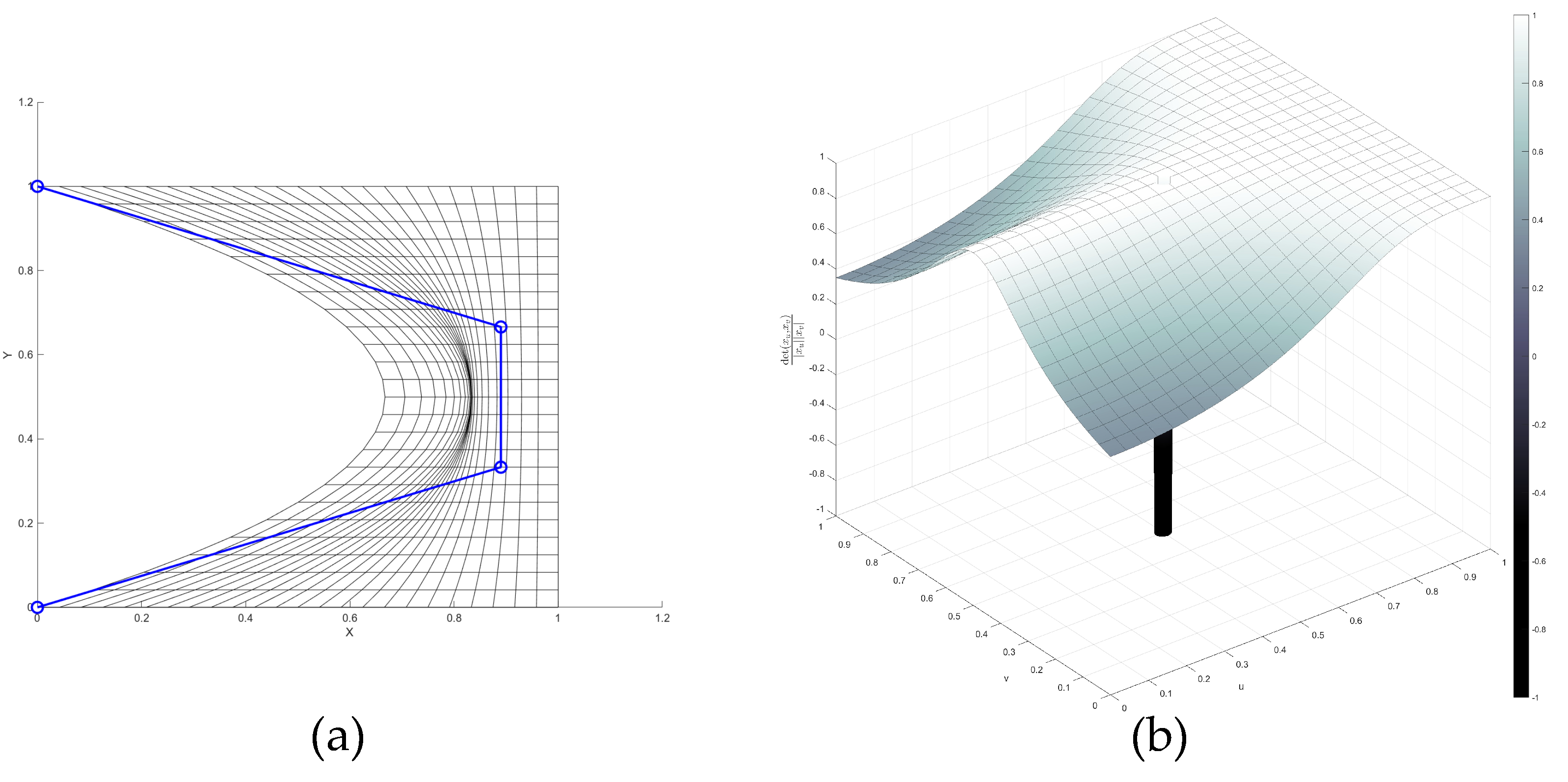
In Figure 11a, the curved side of the parameter space involves the parametrized Bézier points $b_i^3=(i/3, \mu )$, $i=1, 2$ with a parameter $\mu$. Positive values of $\mu$ correspond to a non-convex shape of the parameter region. With the help of our method, we found that $\mathbf{x}$ is regular for $\mu \in [0, 0.88]$. For $\mu \ge 0.89$, $\mathbf{x}$ is not regular. (The investigation was limited to two decimal places.) To visualize the quality of the parametrization, we show a plot of its scaled Jacobian function.

$$\tilde{J}={\displaystyle \frac{\det ({\mathbf{x}}_u,{\mathbf{x}}_v)}{|{\mathbf{x}}_u\left|\right|{\mathbf{x}}_v|}}.$$

Note, that absolute values of $\tilde{J}$ close to 1 indicate the orthogonality of the parameter lines. The non-regularity of this example with $\mu =0.89$ is visible in Figure 12b as a sharp drop of $\tilde{J}$ to zero that occurs when the parametrization folds over. Also note that the plot of the parameter lines cannot be used to judge whether a Coons map is regular, since the plots in Figure 11a and Figure 12a look almost identical.

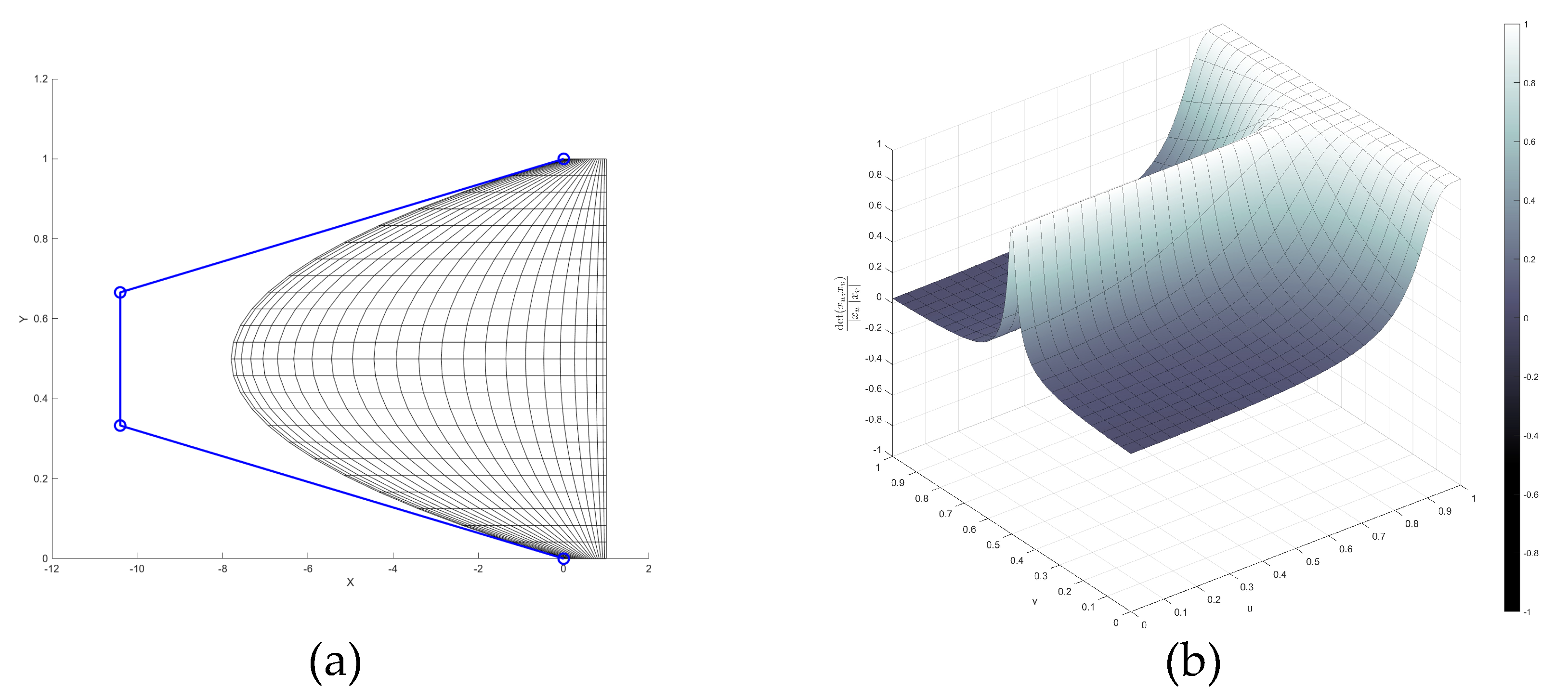
Negative values of $\mu$ correspond to a convex shape of the parameter region and our method verifies that the Coons map is regular in this case. However, for large values of $\mu$, the parametrization gets very uneven. Figure 13a shows the parametrization for $\mu =-10$ and Figure 13b shows the corresponding scaled Jacobian.

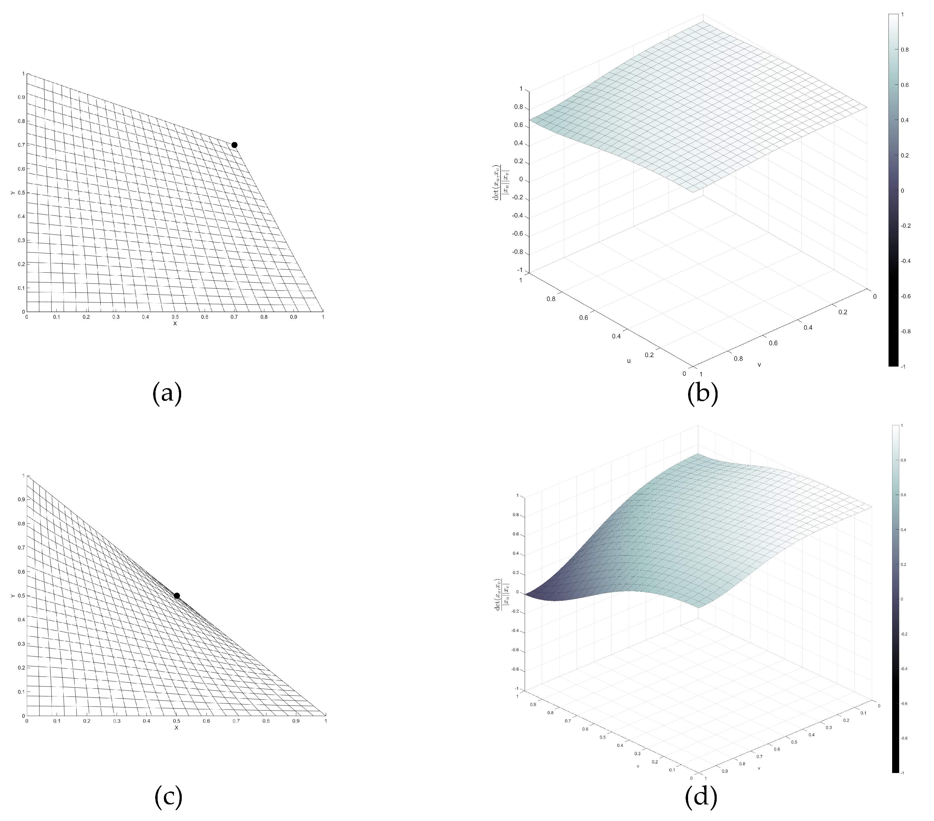
For a convex quadrilateral, we know from Corollary 2 that the associated Coons map is regular. We use this case as a benchmark to see whether our algorithm verifies the regularity, if the shape of the quadrilateral is nearly triangular. Figure 14 shows a parametrized quadrilateral consisting of the vertices $(0, 0), (0, 1), (0, 1), (\nu , \nu )$ where the parameter $\nu >0$ controls the distance of one corner to the origin. From Corollary 2, we know that the map is regular for $\nu >0.5$. In our tests, we received the results that the map is regular for $\nu \ge 0.5+8\times {10}^{-11}$ with $J(1, 1)$ having a very small positive value (see Figure 14d). For smaller values of $\nu$, our algorithm decides that the map is not regular.

Finally, we return to our initial examples introduced in Section 4. For our first example from Figure 7, we already mentioned that $\mathbf{x}$ is regular for $\epsilon \in [0, 0.49]$ (see Figure 8). For $\epsilon \ge 0.5$, $\mathbf{x}$ is not regular. For our example from Figure 9, $\mathbf{x}$ is regular for $\sigma \in [0, 0.35]$. For $\sigma \ge 0.36$, $\mathbf{x}$ is not regular.

7. Conclusions

We have presented an in-depth study of the regularity of a planar Coons map. We found two special cases where the regularity of the Coons map is guaranteed: (a) if opposite boundary curves are parallel translates and (b) if all boundary curves are linear parametrized lines. Combining necessary and sufficient criteria for regularity we presented an algorithm that decides whether an arbitrary planar Coons map is regular. The effectiveness of this algorithm is demonstrated for several parametrized models. With our method, the parameter ranges are determined for which regularity holds.