Article

Economic Peaks and Value-at-Risk Analysis: A Novel Approach Using the Laplace Distribution for House Prices

by
Jondeep Das
1,
Partha Jyoti Hazarika
1,
Morad Alizadeh
2,
Javier E. Contreras-Reyes
3,*,
Hebatallah H. Mohammad
4 and
Haitham M. Yousof
5
1
Department of Statistics, Dibrugarh University, Assam 786004, India
2
Department of Statistics, Faculty of Intelligent Systems Engineering and Data Science, Persian Gulf University, Bushehr 75169, Iran
3
Instituto de Matemática, Física y Estadística, Facultad de Ingeniería y Negocios, Universidad de Las Américas, Sede Viña del Mar, 7 Norte 1348, Viña del Mar 2531098, Chile
4
Department of Mathematical Sciences, College of Science, Princess Nourah bint Abdulrahman University, P.O. Box 84428, Riyadh 11671, Saudi Arabia
5
Department of Statistics, Mathematics and Insurance, Benha University, Benha 13511, Egypt
*
Author to whom correspondence should be addressed.
Math. Comput. Appl. 2025, 30(1), 4; https://doi.org/10.3390/mca30010004
Submission received: 21 November 2024 / Revised: 31 December 2024 / Accepted: 3 January 2025 / Published: 7 January 2025
(This article belongs to the Section Social Sciences)

Abstract

:
In this article, a new extension of the standard Laplace distribution is introduced for house price modeling. Certain important properties of the new distribution are deducted throughout this study. We used the new extension of the Laplace model to conduct a thorough economic risk assessment utilizing several metrics, including the value-at-risk (VaR), the peaks over a random threshold value-at-risk (PORT-VaR), the tail value-at-risk (TVaR), the mean of order-P (MOP), and the peaks over a random threshold based on the mean of order-P (PORT-MOP). These metrics capture different facets of the tail behavior, which is essential for comprehending the extreme median values in the Boston house price data. Notably, PORT-VaR improves the risk evaluations by incorporating randomness into the selection of the thresholds, whereas VaR and TVaR focus on measuring the potential losses at specific confidence levels, with TVaR offering insights into significant tail risks. The MOP method aids in balancing the reliability goals while optimizing the performance in the face of uncertainty.

1. Introduction

According to [1], the dynamics of housing markets are crucial for understanding broader economic trends and stability. As fluctuations in house prices can significantly impact household wealth, consumer confidence, and investment strategies, it is imperative to develop robust statistical models that accurately assess these variations (see also [2]). The study by [1] is an important contribution to the field of real estate economics and predictive modeling [3,4,5]. By systematically comparing regression models for house price predictions in Boston, the authors provide valuable insights that can enhance understanding and decision-making within the housing market. Their work highlights the necessity of continuous advancements in the analytical techniques to keep pace with the complexities of real estate dynamics.
Significant contributions to the field of risk assessment and portfolio management have emerged from a variety of researchers, with each advancing our understanding of financial risk dynamics. Ref. [6] delves into the effects of the thresholds ( T h ) within both expected utility and mean-variance frameworks for asset allocation, emphasizing the importance of recognizing when the losses exceed certain critical levels. This analysis enhances the traditional approaches by integrating threshold effects, which can significantly influence investment decisions and risk management strategies. In [7], the concept of tail risk is expanded by introducing tail value (TV) premiums for elliptical portfolios, thereby broadening the range of risk measures available to investors beyond the conventional value-at-risk (VaR). Their work underscores the necessity of considering tail risk—events that, while rare, can have substantial financial implications. Ref. [8] further builds on this discourse by exploring tail mean variance (TMV) as a criterion for the optimal portfolio selection. This approach offers a more nuanced framework for assessing risk and return, particularly in the presence of extreme market movements. Similarly, ref. [9] suggests the use of expectiles as an alternative to quantiles for estimating the VaR and expected shortfall, providing an innovative perspective on how to quantify the potential losses in uncertain environments. Ref. [10] focuses on loss modeling within the realms of insurance and risk management, presenting methodologies for effectively addressing heavy-tailed distributions and extreme loss scenarios. Their contributions are critical for actuaries and risk managers who must account for infrequent but severe losses in their assessments. Ref. [11] offers a comprehensive guide to modeling extreme events in finance and insurance, serving as an invaluable resource for practitioners seeking to understand the intricacies of tail risks and their implications for financial stability. Other notable research includes studies on the impact of confidence levels in risk assessment [12], as well as analyses of Burr and Pareto distributions [13], which enrich the toolkit available for risk measurement and portfolio optimization. Ref. [14] contributes to the development of portfolio models specifically designed for VaR estimation, enhancing the precision of the risk assessments in financial contexts. Recent advancements have included the functional extensions to portfolio analysis proposed by [15], as well as the introduction of innovative risk models tailored to specific reliability and actuarial applications, such as the XGamma extension [16] and Bayesian risk frameworks [17]. These developments reflect a shift towards more sophisticated methodologies that capture the complexities of financial risks better. Moreover, new models, including the extended Gompertz model [18] and cutting-edge loss probability models [19], signify ongoing progress in refining risk assessment techniques. Together, these studies underscore the importance of employing advanced methods such as the MOP in improving the accuracy and reliability of risk evaluations in financial and economic settings. The integration of these sophisticated approaches not only enhances our understanding of potential risks but also supports more informed decision-making among investors and policymakers, ultimately contributing to greater financial resilience.
On the other hand, the Laplace distribution (Pierre-Simon Laplace, 1749–1827) is considered a location parameter [20] and is also known as the double exponential distribution or two-tailed distribution [21]. Both normal and Laplace distributions are often used to fit symmetric data (and more specifically to fit symmetric data with shorter tails than a normal distribution); however, for long tails, the Laplace distribution is often used. The PDF of Laplace distribution is given as
g ( x ) = 0.5 e x , x 0 0.5 e x , x < 0 .
On the other hand, the CDF of the Laplace distribution is given by
G ( x ) = 1 0.5 e x , x 0 0.5 e x , x < 0 .
With the introduction of the Laplace distribution, several works have been carried out on the development of the Laplace distribution considering different approaches, specially in practical situations when asymmetry arises in the data and where the Laplace distribution does not have a good fit. To asses these issues, ref. [21] proposed an asymmetrical version of the Laplace distribution, adopting the idea of a skew-normal distribution [22]. This new distribution is called the skew-Laplace (SLa) distribution and allows us to fit non-symmetric unimodal data. Later on, continuous research was carried out on the generalization of the SLa distribution to obtain different, new asymmetric Laplace distributions. For example, the alpha skew-Laplace distribution [23], the Balakrishnan alpha beta skew-Laplace distribution [24], and the multimodal skew Laplace distribution [25], among others, are some models which include the SLa distribution from [21] as a special case and fit uni/bimodal as well as multimodal data.
On the other hand, ref. [26] introduced a distinctive class of distributions with an added shape parameter, a > 0 , termed the odd log-logistic-G (OLL-G) family of distributions. Recently, several researchers have extended the odd-log-logistic family, leading to a variety of new distributions. Examples include the generalized odd log-logistic family [27], the odd log-logistic normal (OLLN) distribution [28], the odd log-logistic log normal distribution [29], and the odd log-logistic Student t distribution [30]. Another noteworthy distribution within the OLL family, known as the Kumaraswamy odd log-logistic distribution, was proposed by [31]. Additional advancements include the odd log-logistic logarithmic generated family [32], the exponentiated odd log-logistic family [33], the odd log-logistic exponentiated Weibull distribution [34], and the odd log-logistic Marshall–Olkin power Lindley distribution [35]. Recently, ref. [36] introduced a new variant called the NOLL-G family, expanding on the framework of [37].
Following [1], in this paper, we explore a novel approach to evaluating the economic peaks and the associated risks in house prices using the new odd log-logistic standard Laplace (NOLL-SLa) extension, a statistical model known for its ability to capture the heavy-tailed behavior often observed in financial data. The traditional methods for assessing risk, such as VaR and TVaR, PORT-VaR, MOP, and PORT-MOP, atypically rely on normal distribution assumptions, which may not adequately reflect the complexities of real estate markets. This research aims to demonstrate the efficacy of the Laplace distribution in modeling house price dynamics, particularly in the presence of extreme events and economic peaks. By applying this innovative approach, we provide insights into the predictive power of the Laplace distribution and its implications for risk management and investment decisions. Through an extensive empirical analysis of housing data, we investigate the characteristics of the house price distributions and the frequency of extreme fluctuations. Our findings contribute to a deeper understanding of market behavior and offer valuable tools for policymakers and investors navigating the complexities of the real estate sector (see [38,39] for more details).
Therefore, this article introduces a new family of Laplace distributions based on the mechanism of [36]. This study also includes some important statistical properties of the new distribution, along with some graphical illustrations of the cumulative distribution (CDF) and probability distribution (PDF) functions. A location and scale extension of the newly proposed PDF is also included throughout the study of the parameter estimation. Further, a simulation study is conducted to observe the performance of the estimated parameters of the new distribution. Finally, the flexibility, adaptability, and usefulness of the new distribution are thoroughly checked using house price datasets. Comparisons with other existing models are made using the Akaike information (AIC) and Bayesian information (BIC) criteria. Further, a thorough economic risk assessment utilizing several metrics for this new model is also presented.

2. The New Odd Log-Logistic Standard Laplace Distribution

In this section, the CDF and PDF of the new distribution are defined and graphically presented.
Definition 1.
A random variable X is said to follow the NOLL-SLa distribution if its CDF is given as
F ( x ) = G ( x ) a G ( x ) a + 1 G ( x ) b ,
where a , b > 0 , and G ( x ) and g ( x ) denote the CDF and PDF of the standard Laplace distribution, respectively. The proposed distribution is denoted as NOLLSLa ( a , b ) .
Definition 2.
The corresponding PDF of the NOLLSLa ( a , b ) distribution is derived as
f ( x ) = g ( x ) G ( x ) a 1 [ 1 G ( x ) ] b 1 [ a + ( b a ) G ( x ) ] G ( x ) a + [ 1 G ( x ) ] b 2 ,
where a , b > 0 , and G ( x ) and g ( x ) denote the CDF and PDF of the standard Laplace distribution, respectively.
Proof. 
It is simple to obtain (1) from (2).    □
Remark 1.
Some special cases of the NOLLSLa ( a , b ) distribution are given as follows:
i. 
For a = b , we obtain the odd log-logistic standard Laplace distribution;
ii. 
For a = b = 1 , we obtain the standard Laplace distribution.
The PDF of the NOLLSLa( a , b ) distribution is depicted in Figure 1 for different values of the parameter. Similarly, Figure 2 shows the plots of the CDF of the NOLLSLa( a , b ) distribution for different choices of the parameter. In the graphical illustration, the location and scale parameters for the new distribution are assumed to be 0 and 1, respectively. From Figure 1, it is clear that the left tail of the PDF depends only on parameter a, while the right tail of the PDF depends only on parameter b. Again, for a = b = 1 , the new distribution is reduced to the standard Laplace distribution (see Figure 1d), while for a = b , the new distribution is reduced to the odd log-logistic standard Laplace distribution (see Figure 1c).

3. Main Properties

This section includes some important mathematical properties of the NOLLSLa ( a , b ) distribution.

3.1. Asymptotics

The asymptotics of the CDF and the PDF as x are given as
F ( x ) e x 2 a , f ( x ) a e x 2 a .
The asymptotics of the CDF and the PDF as x are given as
1 F ( x ) e x 2 b , f ( x ) b e x 2 b .
It can be observed that for x , the asymptotics of the CDF and the PDF only depends on parameter a (i.e., a smaller value for a results in heavier tails, while a larger value for a results in lighter tails). Therefore, both the PDF and the CDF in the left tail depend only on parameter a (see Figure 1 and Figure 2). On the other hand, for x , the asymptotics of the CDF and the PDF only depend on parameter b (i.e., the tail becomes heavier when b is small and becomes lighter when b is large). Hence, both the PDF and the CDF in the right tail depend only on parameter b (see Figure 1 and Figure 2). In other words, | f ( x ) f a s m ( x ) | 0 for x ± and | F ( x ) F a s m ( x ) | 0 for x ± , where f a s m ( x ) and F a s m ( x ) are the asymptotics of the PDF and the CDF of the new distribution, respectively. Again, the asymptotic results for the CDF and the PDF provide a good approximation for sufficiently small values of x in the left tail, while in the right tail, the asymptotic results of CDF and PDF provide a good approximation for large values of x.

3.2. Linear Combinations for the CDF and PDF

First, note that
G ( x ) a = 1 ( 1 G ( x ) ) a = l = 0 ( 1 ) l a l 1 G ( x ) l = l = 0 m = 0 l ( 1 ) l + m a l l m G ( x ) m = m = 0 l = m l ( 1 ) l + m a l l m G ( x ) m = m = 0 a m G ( x ) m ,
where
a m = l = m l ( 1 ) l + m a l l m .
Also,
G ( x ) a + 1 G ( x ) b = m = 0 b m G ( x ) m ,
where b m = a m + ( 1 ) m b m ; then,
F ( x ) = m = 0 a m G ( x ) m m = 0 b m G ( x ) m .
Using the ratio of two power series, we can write
F ( x ) = m = 0 a m G ( x ) m m = 0 b m G ( x ) m = m = 0 λ m G ( x ) m ,
where λ 0 = a 0 b 0 , and for m 1 , we have
λ m = 1 b 0 a m 1 b 0 r = 1 m a r b m r .
The following equation shows that the CDF of the NOLLSLa ( a , b ) distribution can be written as a linear combination of exponentiated standard Laplace distributions.
f ( x ) = m = 1 m λ m g ( x ) G ( x ) m 1 = m = 1 m λ m e x 2 m , x 0 m = 1 m λ m e m x j = 1 m 1 2 j , x > 0 .

3.3. Moments and Incomplete Moments

Theorem 1.
The n-th-order moment of NOLLSLa( a , b ) distribution is obtained as
E ( X r ) = Γ ( r + 1 ) m = 1 ( 1 ) r λ m 2 m m r + m = 1 j = 0 m 1 λ m 2 j + 1 m r ,
where Γ ( a ) = 0 z a 1 e z d z denotes the gamma function.
Proof. 
0 x r f ( x ) d x = m = 1 m λ m 2 m 0 x r e m x d x = Γ ( r + 1 ) m = 1 ( 1 ) r λ m 2 m m r .
And
0 x r f ( x ) d x = m = 1 m λ m 0 x r e m x d x j = 1 m 1 2 j = Γ ( r + 1 ) m = 1 λ m m r j = 1 m 1 2 j .
Adding the last two results obtained for x 0 and x > 0 , the final expression for the r-th-order moment of the NOLLSLa( a , b ) distribution is obtained.    □
Remark 2.
Putting r = 1 , 2 , 3 , 4 into (10), the first four r-th-order moments of the NOLLSLa( a , b ) distribution are obtained as
E ( X ) = m = 1 λ m 2 m m + m = 1 j = 0 m 1 λ m 2 j + 1 m E ( X 2 ) = m = 1 λ m 2 m 1 m 2 + m = 1 j = 0 m 1 λ m 2 j m 2 E ( X 3 ) = m = 1 3 λ m 2 m 1 m 3 + m = 1 j = 0 m 1 3 λ m 2 j m 3 E ( X 4 ) = m = 1 3 λ m 2 m 3 m 4 + m = 1 j = 0 m 1 3 λ m 2 j 2 m 4 .
Theorem 2.
The r-th-order incomplete moment of the NOLLSLa ( a , b ) distribution is obtained as
m r ( y ) = 1 F ( y ) m = 1 [ m λ m 2 m ( 1 ) r m r + 1 Γ ( r + 1 ) m r 1 Γ ( r + 1 , m y ) r Γ ( r ) + j = 0 m 1 m λ m 2 j + 1 ( 1 ) r ( m ) r + 1 Γ ( r + 1 ) + m r 1 Γ ( r + 1 ) Γ ( r + 1 , m y ) ] ;
for y > 0 , and
m r ( y ) = 1 F ( y ) m = 1 [ m λ m 2 m ( 1 ) r m r + 1 Γ ( r + 1 ) + m r 1 Γ ( r + 1 , m y ) r Γ ( r ) + j = 0 m 1 m λ m 2 j + 1 ( 1 ) r ( m ) r + 1 Γ ( r + 1 ) m r 1 Γ ( r + 1 ) Γ ( r + 1 , m y ) ] ,
for y < 0 .
Proof. 
The incomplete moment of the NOLLSLa( a , b ) distribution is given by
m r ( y ) = E X r | X < y = 1 F ( y ) y x r f ( x ) d x .
For y > 0 ,
m r ( y ) = E X r | X < y = 0 x r f ( x ) d x + 0 y x r f ( x ) d x = 1 F ( y ) m = 1 [ m λ m 2 m 0 x r e m x d x + 0 y x r e m x d x + j = 0 m 1 m λ m 2 j + 1 0 x r e m x d x + 0 y x r e m x d x ] = 1 F ( y ) m = 1 [ m λ m 2 m ( 1 ) r m r + 1 Γ ( r + 1 ) m r 1 Γ ( r + 1 , m y ) r Γ ( r ) + j = 0 m 1 m λ m 2 j + 1 ( 1 ) r ( m ) r + 1 Γ ( r + 1 ) + m r 1 Γ ( r + 1 ) Γ ( r + 1 , m y ) ] .
For y < 0 ,
m r ( y ) = E X r | X < y = 0 x r f ( x ) d x 0 y x r f ( x ) d x = 1 F ( y ) m = 1 [ m λ m 2 m 0 x r e m x d x + 0 y x r e m x d x j = 0 m 1 m λ m 2 j + 1 0 x r e m x d x + 0 y x r e m x d x ] = 1 F ( y ) m = 1 [ m λ m 2 m ( 1 ) r m r + 1 Γ ( r + 1 ) + m r 1 Γ ( r + 1 , m y ) r Γ ( r ) + j = 0 m 1 m λ m 2 j + 1 ( 1 ) r ( m ) r + 1 Γ ( r + 1 ) m r 1 Γ ( r + 1 ) Γ ( r + 1 , m y ) ] .
   □

3.4. The Moment Generating Function

Theorem 3.
The moment generating function (MGF) of the NOLL-L ( a , b ) distribution is given by
M ( t ) = m = 1 m λ m 2 m ( m + t ) + m = 1 j = 0 m 1 m λ m 2 j + 1 ( m t ) .
Proof. 
For x 0 ,
M ( t ) = 0 e x t f ( x ) d x = m = 1 m λ m 2 m 0 e x t e m x d x = m = 1 m λ m 2 m ( m + t ) .
For x > 0 ,
M ( t ) = 0 e x t f ( x ) d x = m = 1 j = 0 m 1 m λ m 2 j + 1 0 e x t e m x d x = m = 1 j = 0 m 1 m λ m 2 j + 1 ( m t ) .
Adding the two results obtained for x 0 and x > 0 , the final expression for the MGF of the NOLLSLa( a , b ) distribution is obtained.    □
Remark 3.
Replacing t with i t in (13), the characteristic function (CF) of the NOLLSLa( a , b ) distribution is
ϕ ( t ) = m = 1 m λ m 2 m ( m + i t ) + m = 1 j = 0 m 1 m λ m 2 j + 1 ( m i t ) .
Remark 4.
Applying log on both sides of (13), the cumulant generating function (CGF) of the NOLLSLa( a , b ) distribution is
K ( t ) = m = 1 m λ m 2 m ( m + i t ) + m = 1 j = 0 m 1 m λ m 2 j + 1 ( m i t ) .

3.5. Mean Deviation

Theorem 4.
The mean deviation om the NOLLSLa ( a , b ) distribution about the mean μ is obtained as
δ 1 ( x ) = 2 μ F ( μ ) 2 m 1 ( μ ) F ( μ ) ,
where m 1 ( μ ) is defined using the expression for the incomplete moment of the NOLLSLa ( a , b ) distribution in (11) and (12).
Proof. 
One partial measure of the degree of dispersion within a population is the sum of the departures from the mean and the median. The following definitions apply to these deviations, which are also known as the mean deviation about the mean and the mean deviation about the median:
δ 1 ( X ) = | x μ | f ( x ) d x ,
δ 2 ( X ) = | x M | f ( x ) d x ,
respectively, where μ = E ( X ) , and M denotes the median. Therefore, δ 1 ( X ) can be calculated as
δ 1 ( X ) = | x μ | f ( x ) d x = 2 μ F ( μ ) 2 μ x f ( x ) d x = 2 μ F ( μ ) 2 I 1 .
Now, from the results of the incomplete moments for the NOLLSLa ( a , b ) distribution mentioned in (11) and (12), I 5 can be written as
I 1 = m = 1 [ m λ m 2 m 2 m 2 + m 2 Γ ( 2 , m y ) 1 + j = 0 m 1 m λ m 2 j + 1 2 m 2 + m 2 1 Γ ( 2 , m y ) ] ,
for μ > 0 . For μ < 0 ,
I 1 = m = 1 [ m λ m 2 m 2 m 2 + m 2 Γ ( 2 , m y ) 1 + j = 0 m 1 m λ m 2 j + 1 2 m 2 m 2 2 Γ ( 2 , m y ) ] .
Hence, the final result for the mean deviation about the mean for the N O L L S L a ( a , b ) distribution is obtained as δ 1 ( x ) = 2 μ F ( μ ) 2 m 1 ( μ ) F ( μ ) .    □
Remark 5.
Replacing the mean μ with the median M in (16), the mean deviation in the N O L L S L a ( a , b ) distribution about the median M, i.e., δ 2 ( X ) , can be obtained.

3.6. Order Statistics

Theorem 5.
The PDF of the k-th-order statistics for the N O L L S L a ( a , b ) distribution is given as
f i : n ( x ) = k = i n i = 0 n k ( 1 ) l n k n k l A s g ( x ) G ( x ) a ( k + l ) ( k + l p + q ) 1 ,
where A s = [ p = 0 k + l q = 0 ( 1 ) q ] 1 and
G ( x ) = { 0.5 e x , x 0 ; 1 e x 2 , x > 0 .
Proof. 
Assume that a random sample X 1 , X 2 , , X n was taken from (2). Assume once more that the associated order statistic is X 1 : n < X 2 : n < < X n : n . Then, the CDF of the k-th-order statistic may be defined as
F i : n = k = i n n k F ( x ) k 1 F ( x ) k = k = i n i = 0 n k ( 1 ) l n k n k l F ( x ) k + l = k = i n i = 0 n k ( 1 ) l n k n k l G ( x ) a G ( x ) a + 1 G ( x ) b k + l .
Now,
G ( x ) a + ( 1 G ( x ) ) b k + l = p = 0 k + l G ( x ) k + l p ( 1 G ( x ) ) b p = p = 0 k + l G ( x ) k + l p × q = 0 ( 1 ) q b p q G ( x ) q = p = 0 k + l q = 0 ( 1 ) q G ( x ) k + l p + q
Hence,
F i : n = k = i n i = 0 n k ( 1 ) l n k n k l G ( x ) a ( k + l ) p = 0 k + l q = 0 ( 1 ) q G ( x ) k + l p + q = k = i n i = 0 n k ( 1 ) l n k n k l A s G ( x ) a ( k + l ) ( k + l p + q ) ,
where A s = [ p = 0 k + l q = 0 ( 1 ) q ] 1 . Then, the PDF of the k-th-order statistic of the N O L L S L a ( a , b ) distribution is obtained as
f i : n ( x ) = d F i : n ( x ) d x = k = i n i = 0 n k ( 1 ) l n k n k l A s g ( x ) G ( x ) a ( k + l ) ( k + l p + q ) 1 .
   □

3.7. Quantiles and the Pseudo-Random Generator

Property 1.
Let X N O L L S L a ( a , b ) . Then, the p-th ( 0 < p < 1 ) quantile is a solution of the equation
G ( x p ) a p G ( x p ) a + 1 G ( x p ) b = 0
Proof. 
Equation (17) is easy to obtain based on (1).    □
Property 2.
Let R U ( 0 , 1 ) . The pseudo-random number generator of X is a solution of the equation
G ( X ) a R G ( X ) a + 1 G ( X ) b = 0 .
Proof. 
If R U ( 0 , 1 ) , then ( 1 R ) U ( 0 , 1 ) . Equation (18) is easy to obtain based on (17). 
   □

4. Parameter Estimation

This section concerns the parameter estimation of the N O L L S L a ( a , b ) distribution. Firstly, an extension of the N O L L S L a ( a , b ) distribution is proposed considering the location parameter μ and the scale parameter σ > 0 . The new PDF is denoted as N O L L S L a ( μ , σ , a , b ) , and it is given by
f ( x ; μ , σ , a , b ) = g ( x ; μ , σ ) G ( x ; μ , σ ) a 1 [ 1 G ( x ; μ , σ ) ] b 1 [ a + ( b a ) G ( x ; μ , σ ) ] G ( x ; μ , σ ) a + [ 1 G ( x ; μ , σ ) ] b 2 ,
where g ( x ; μ , σ ) = 1 2 σ exp x μ σ ,
G ( x ; μ , σ ) = 1 + S i g n x μ b 1 exp x μ σ 2
and S i g n ( x ) gives –1, 0, or 1 depending on whether x is negative, zero, or positive.
Now, consider a collection of n independent, identically distributed random variables, y 1 , y 2 , y 3 , , y n , that are derived from the NOLLSLa ( μ , σ , a , b ) distribution. Then, the log-likelihood function is obtained as follows:
l ( θ ) = i = 1 n y i μ σ + ( a 1 ) i = 1 n log G ( y i ; μ , σ ) + ( b 1 ) i = 1 n log 1 G ( y i ; μ , σ ) + i = 1 n log a + ( b 1 ) G ( y i ; μ , σ ) 2 i = 1 n log G ( y i ; μ , σ ) a + ( 1 G ( y i ; μ , σ ) ) b .
Differentiating Equation (20) with respect to each parameter, the derivatives of the log-likelihood function are
l ( θ ) μ = i = 1 n 2 a ( b + a μ a y i ) b 2 1 + E ( 1 ) ) + i = 1 | n | y i μ | b i = 1 n E ( 1 ) ( b a ) 1 + E ( 2 ) 2 E ( 3 ) σ , l ( θ ) σ = n σ + b σ i = 1 n y i μ σ i = 1 n 2 a ( y i μ ) ( b + a μ a y i ) b 3 E ( 2 ) + i = 1 | n | y i μ | b 2 , l ( θ ) a = i = 1 n a + b e y i μ σ 1 + n b i = 1 n ( y i b E ( 1 ) b 2 + a b 2 i = 1 n | y i μ | , l ( θ ) b = i = 1 n b + a e μ y i σ 1 i = 1 n y i μ σ i = 1 n log e y i μ σ + 1 2 i = 1 n E ( 1 ) a μ σ log E ( 1 ) y i σ E ( 4 ) ,
where E ( 1 ) = | y i μ σ | + 1 , E ( 2 ) = exp ( y i / σ ) + exp ( μ / σ ) , E ( 3 ) = exp b μ + b y i + μ σ , and E ( 4 ) = E ( 1 ) a + exp ( ( y i μ ) b σ ) E ( 1 ) .
One can now acquire the estimations by simultaneously solving the aforementioned equations. However, the aforementioned normal equations do not have an explicit direct solution. As a result, a numerical procedure can be built using the GenSA library in R software version 4.4.1.

5. The Simulation Study

Simulation research was carried out to assess the efficacy of the MLEs of θ = ( μ , σ , a , b ) . Careful consideration was given to how sensitive the simulation process was to the starting parameters θ s = ( μ , σ , a , b ) . The initial value for μ was chosen from the interval μ s ( μ 0.25 , μ + 0.25 ) , and those for the remaining parameters were chosen from θ ¯ s ( θ ¯ 0.25 , θ ¯ + 0.25 ) , where θ ¯ = ( σ , a , b ) , to avoid the estimation problems that occur when the initial values coincide with the input values of the pseudo-random number generator. The mean squared errors (MSEs) and biases of the estimations are used to provide the estimated statistics (see Table 1 and Table 2). The MSE and biases are defined as
B i a s ( θ ^ ) = E ( θ ^ ) θ , M S E ( θ ^ ) = V ( θ ^ ) + B i a s ( θ ^ ) 2 ,
respectively, where θ ^ = ( μ ^ , σ ^ , a ^ , b ^ ) . The simulation study was performed with 10 3 samples using sample sizes n = 100 , 300, and 500. The samples were drawn from the NOLL-L ( 0 , 1 , a , b ) distribution, where a and b take specific values. We note that the approximations become closer to the actual numbers; thus, an increment in the sample size indicates that the estimations are consistent.

6. The Boston Dataset

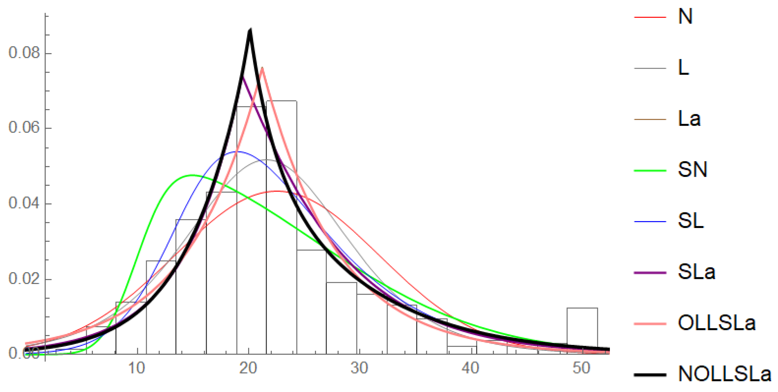
In this section, the applicability and adaptability of the proposed distribution are checked against competitor models. For this comparison, the standard normal distribution (N), standard logistic distribution (L), standard Laplace distribution ( L a ), skew-normal distribution ( S N ) [22], skew-logistic distribution ( S L ) [40], skew-Laplace distribution ( S L a ) [41], and odd log-logistic standard Laplace distribution ( O L L S L a ) (mentioned in Remark 1) are considered. The Akaike information criterion (AIC) and the Bayesian information criterion (BIC) are used for the comparisons.
The Boston dataset contains the median values of house prices (medv) in n = 506 neighborhoods around Boston and was previously analyzed by [42]. The results on the maximum likelihood estimators (MLEs), log-likelihood, AIC, and BIC of the models are reported in Table 3.
From Table 3, it is clear to see that the new distribution is more appropriate and better fitted compared to the other competitors in terms of the log-likelihood, AIC, and BIC. The flexibility of the new distribution is also visualized in Figure 3.
Since L a , O L L S L a , and N O L L S L a are nested models, therefore, to discriminate between them, the likelihood ratio (LR) test is used. The test statistics as well as the null hypothesis of the test are as follows:
(i)
To discriminate the L a distribution from the N O L L S L a distribution, the null hypothesis H 0 : a = 0 , b = 0 is tested against the alternative hypothesis H 1 : a 0 , b 0 . The test statistic is
2 log ( L R ) = 2 [ log L ( μ ^ 1 , σ ^ 1 , a = b = 0 | x ) log L ( μ ^ 2 , σ ^ 2 , a ^ 2 , b ^ 2 ) ] χ 2 2 ,
where ( μ ^ 1 , σ ^ 1 ) and ( μ ^ 2 , σ ^ 2 , a ^ 2 , b ^ 2 ) are, respectively, the MLEs of the L a distribution and the N O L L S L a distribution, and r = 2 is the difference between the numbers of parameters.
(ii)
To discriminate the O L L S L a distribution from the N O L L S L a distribution, the null hypothesis H 0 : b = 0 is tested against the alternative hypothesis H 1 : b 0 . The test statistic is
2 log ( L R ) = 2 [ log L ( μ ^ 1 , σ ^ 1 , a ^ 1 , b = 0 | x ) log L ( μ ^ 2 , σ ^ 2 , a ^ 2 , b ^ 2 ) ] χ 1 2 ,
where ( μ ^ 1 , σ ^ 1 , a ^ 1 ) and ( μ ^ 2 , σ ^ 2 , a ^ 2 , b ^ 2 ) are, respectively, the MLEs of the O L L S L a distribution and the N O L L S L a distribution, and r = 1 is the difference between the numbers of parameters.
From Table 4, it can be noted that the value of the LRT statistics is higher than the tabulated critical value at the 95 % confidence level for datasets I and II. Consequently, it can be stated that the collected data originate from the N O L L S L a ( μ , σ , a , b ) distribution.

7. Risk Indicators

The importance of VaR and TVaR, PORT-VaR, MOP, and PORT-MOP in analyzing the median values in the Boston house price data lies in their ability to provide a comprehensive framework for understanding the financial risk and price dynamics in real estate markets. VaR quantifies the potential losses at a specified confidence level, helping stakeholders to assess the maximum expected declines in property values. PORT-VaR focuses on extreme losses that exceed a predefined threshold, offering insights into tail risks that can significantly impact the housing market. TVaR enhances this by measuring the expected losses in extreme scenarios, crucial for understanding market volatility. Meanwhile, MOP allows for the examination of various statistical moments, providing a nuanced view of both central trends and extreme fluctuations in house prices. Combining these methods, PORT-MOP enables a detailed analysis of the average behavior of extreme values beyond a threshold, enhancing insights into the risk profiles associated with high-value properties. Together, these methodologies support informed decision-making for investors and policymakers, contributing to a more resilient real estate market.

7.1. The VaR q

The VaR at a given confidence level q (typically 0.95, related to 95% confidence) is defined as value x where Pr ( X x ) = q . This requires solving the equation q = F ( x ) . For values of x 0 , the non-negative segment of F ( x ) is used.

7.2. The TVaR q

The TVaR of a random variable X, often denoted as TVaR q , is a crucial measure in risk management and financial analysis. By definition, it is calculated using the following formula.
TVaR q = 1 1 VaR q I VaR q ; | q ,
where
I VaR q ; | q = VaR q x f x d x .
The term TVaR q represents the value-at-risk at a given confidence level q. It quantifies the maximum expected loss over a specified time frame given a certain confidence level. For example, a VaR at the 95% confidence level indicates that there is a 5% chance that losses will exceed this value. The integral in (21) can be tackled using numerical methods to obtain suitable approximate solutions, as obtaining a closed-form expression presents significant challenges. For additional applications and insights, see the works of [8,43]. Then, we have
I VaR q ; | q = I ; | q I ; VaR q | q .
The integration I ; | q is presented in (10) for n = 1 (refer to Remark 3). In contrast, the integration I ; VaR q | q is detailed in (12) for n = 1 and corresponds to the first incomplete moment.

7.3. The MOP Method

As emphasized in the studies by [18,44,45], varying the MOP facilitates a more thorough analysis. This methodology is often employed across multiple values of P (where P = 1 , 2 , 3 , ) to evaluate the impact of different moments on the dataset. Such multi-order analysis is particularly crucial in finance, where it is vital to grasp both central tendencies and extreme risks for informed decision-making. The MOP is defined as
MO P = 1 n i = 1 n x i P 1 P .

7.4. The PORT-VaR

Due to [46], the PORT-VaR method is a crucial instrument in economic risk analysis, particularly for assessing extreme risks and tail events. It enhances the traditional VaR framework, which measures the potential decline in a portfolio’s value over a defined time period at a specified confidence level. The procedure for calculating PORT-VaR consists of the following steps:
  • The selection of T h based on empirical data or expert judgment;
  • Identify exceedances: Filter the dataset to isolate values that surpass the established threshold T h ;
  • Count exceedances: Calculate the total number of exceedances that have been identified;
  • Estimate the empirical CDF for the identified exceedances;
  • Calculate the VaR: Use the empirical distribution of the exceedances to ascertain the VaR at the specified quantile q.
This systematic approach allows for a deeper understanding of tail risks, enabling better-informed decision-making in risk management (see [18,44] for more applications).

8. MOP Analysis for the Median Values of Boston House Price Data

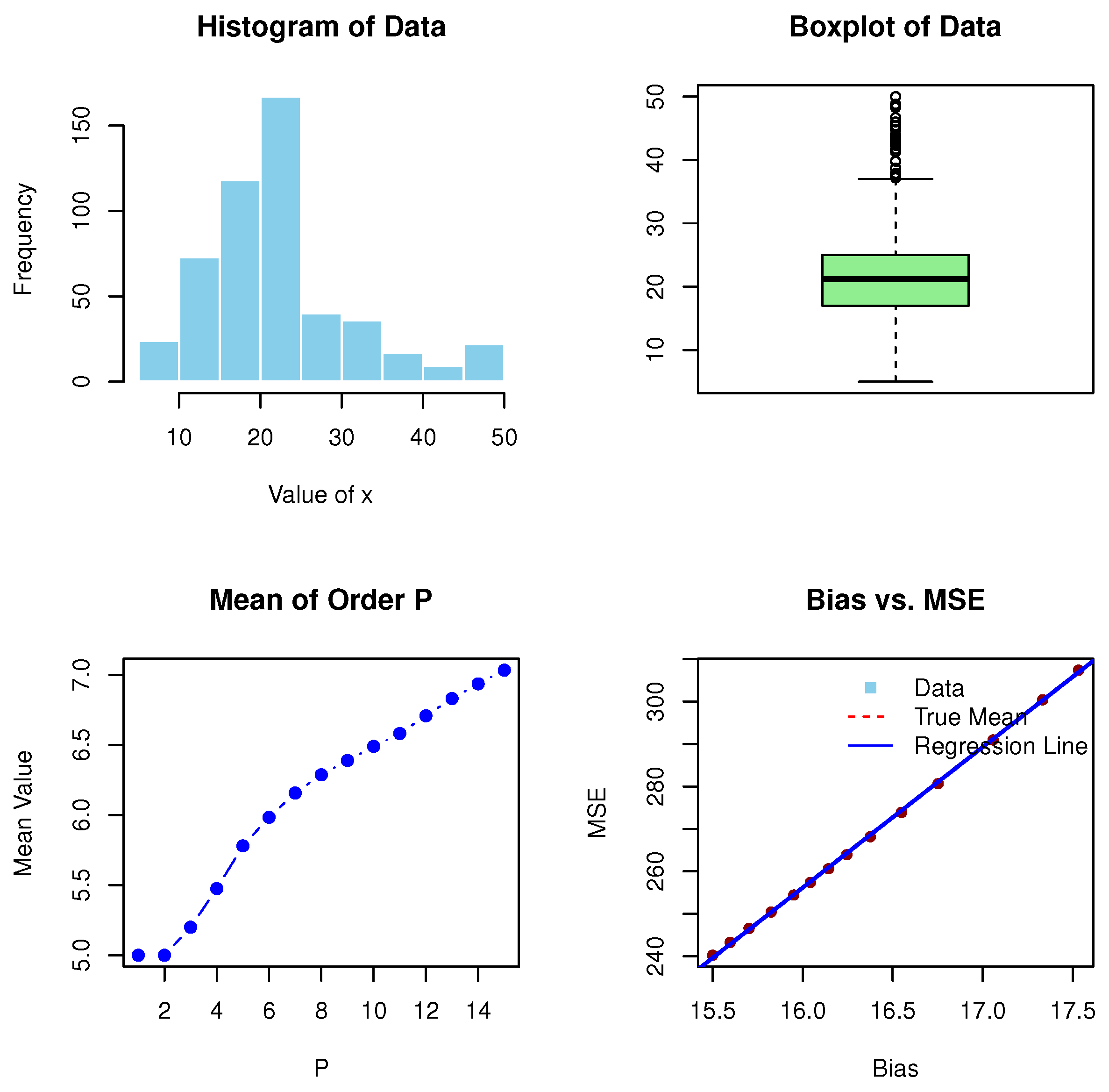
The results presented in Table 5 offer valuable insights into the assessment of the MOP under varying parameter levels P for the median values of Boston house prices. The table provides three key metrics, MOP, mean squared error (MSE), and bias, which collectively inform us about the reliability and performance of the model in predicting housing prices. As we increase P from 1 to 15, the values of MOP exhibit a consistent upward trend, rising from 5.0 at P = 1 to approximately 7.03 at P = 15 . This increase suggests that the profitability, or returns, associated with house prices is improving as we consider higher thresholds. This trend could reflect a positive sentiment in the housing market, indicating that as parameters increase, the potential for greater returns on investment in real estate also rises. In contrast to the rising MOP, the MSE demonstrates a declining pattern, starting at 307.3993 for P = 1 and decreasing to 240.2337 by P = 15 . This reduction in the MSE suggests that the model becomes more accurate in predicting house prices as P increases. A lower MSE indicates that the estimates of house prices are converging more closely to the actual market values, which is crucial for investors and policymakers in the real estate sector. The bias values show a corresponding decrease from 17.53 at P = 1 to 15.50 at P = 15 . This decline indicates that the model is progressively reducing its systematic error in predicting housing prices. Lower bias values enhance the credibility of the model, implying that it can be a reliable tool for assessing housing market dynamics.
Figure 4 provides a comprehensive visual representation through histogram plots, box plots, the MOP values for P = 1 , 2, …, 15, and a comparison of the bias against the MSE for the median values in the Boston house price data. These visualizations are crucial for understanding the distribution of and variability in housing prices, which have significant implications for the broader economic landscape. Figure 4 presents the MOP values across the parameter range. The left panel emphasizes the increasing trend in MOP as P rises, suggesting that higher parameters yield greater returns on investment in the housing market. This trend indicates that as housing prices stabilize, investors might see better profitability in longer-term investments, which could encourage more construction and renovation projects.
Increased investment in housing not only benefits developers and homeowners but also has a multiplier effect on the economy through job creation in related sectors such as construction, finance, and retail. Accurate forecasting of housing prices is essential for economic stability; it allows financial institutions to make informed lending decisions, thereby enhancing liquidity in the housing market.
These findings in Figure 4 and Table 6 have significant implications for the US economy, particularly in the context of the housing market. As house prices stabilize and the prediction models improve, consumer confidence may rise, positively affecting economic growth. Furthermore, with a lower MSE and bias, financial institutions may rely more heavily on such models for risk assessment and lending decisions, fostering a healthier economic environment. A robust housing market often translates into broader economic stability, influencing job creation and consumer spending.

9. The PORT-VaR Estimator for the Median Values in Boston House Price Data

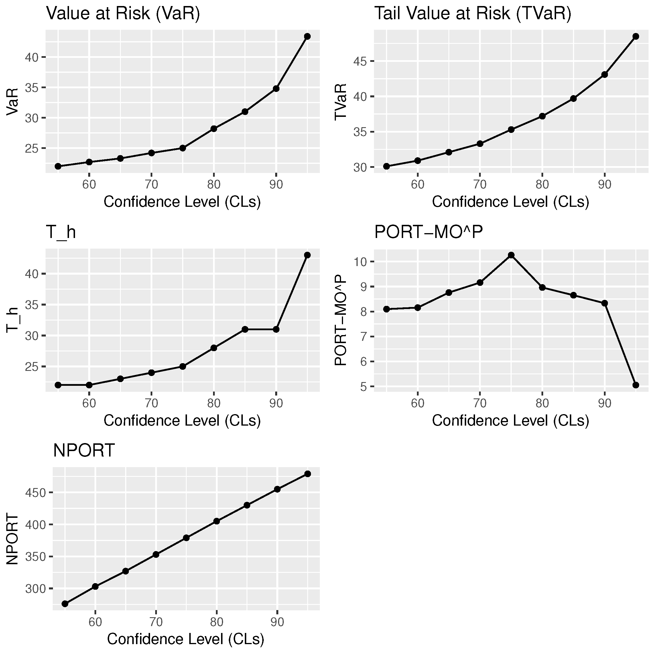
The results in Table 6 present a comprehensive analysis of the VaR, TVaR, and peaks over a random threshold based on the mean of order-P (PORT-MOP) for the median values of Boston house prices. These metrics are crucial for understanding the potential risks associated with housing investments and their broader implications for the US economy. The VaR values show a steady increase as the confidence level (CL) rises, from 22.0 at 55% to 43.4 at 95%. This trend indicates that higher confidence levels correspond to greater potential losses, reflecting the inherent volatility and risk associated with housing investments. For investors and financial institutions, these figures provide a quantitative measure of risk, aiding in portfolio management and decision-making processes.
Understanding the potential losses at varying confidence levels allows stakeholders to adopt more informed strategies, potentially mitigating adverse impacts on the economy during market downturns. The TVaR values also exhibit an upward trend, ranging from 30.1 at a 55% CL to 48.5 at a 95% CL. This increase underscores the severity of potential losses in extreme scenarios. For policymakers and economic analysts, the TVaR metric serves as an essential tool for assessing systemic risks within the housing market. As extreme fluctuations in housing prices can have cascading effects on the broader economy, understanding these risks is vital for ensuring financial stability. High TVaR values indicate that in the worst-case scenarios, losses could significantly impact household wealth and consumer confidence, leading to reduced spending and slower economic growth. The threshold after the VaR ( T h ) values, which reflects the threshold after which losses exceed the VaR, also demonstrates a general increase alongside the confidence levels. This suggests that as the risk threshold rises, the potential for extreme losses increases as well. The implication for the US housing market is profound: if prices begin to decline significantly beyond these thresholds, it could signal a more extensive market correction. Such corrections can lead to decreased construction activity, job losses in the construction sector, and lower consumer spending, all of which are detrimental to the economy. The PORT-MOP values reflect the average of the peaks that exceed a given threshold, ranging from 8.0950 at a 55% CL to 10.2590 at a 75% CL, before declining at higher confidence levels. This fluctuation suggests that while there may be opportunities for high returns in certain scenarios, the risk of encountering extreme price peaks remains significant. Understanding this dynamic is crucial for investors seeking to navigate potential market volatility and capitalize on upward trends in house prices without exposing themselves to excessive risk. The number of peaks over a random threshold (NPORT) values illustrate the frequency of significant price peaks, increasing steadily from 276 at a 55% CL to 479 at a 95% CL. This growth indicates the rising occurrence of extreme fluctuations in house prices, which can signal heightened volatility in the market. For the broader economy, an increase in the NPORT may suggest that the housing market is experiencing more frequent and severe disruptions. Such volatility can deter investment and lead to cautious consumer behavior, potentially stalling economic recovery and growth.
The summary statistics provided, including the minimum (Min), first quartile (1st Qu.), median (Med), expected value (ExV), third quartile (3rd Qu.), and maximum values, reveal important insights into the distribution of the dataset related to Boston house prices.
Starting with the minimum values, we observe a declining trend from 20.50 to 10.40 as the confidence level increases. This indicates that as the confidence level rises, the lowest observed prices in the dataset also decrease, suggesting a potential contraction in the lower end of the housing market. The quartiles and median values, which reflect the central tendency of the dataset, also show a gradual decline across the various confidence levels. For example, the median price drops from 24.70 to 21.70, highlighting a decreasing trend in the typical house prices as we consider higher confidence intervals. This could imply that at higher confidence levels, the market is likely experiencing downward pressure on home values, potentially due to economic factors or market volatility. The ExV presents a similar pattern, starting at 28.37 and falling to 23.35, further indicating that the overall average value of properties decreases with increasing confidence levels. This suggests that in more conservative assessments, we are seeing a more cautious valuation of house prices. Interestingly, the maximum (Max) value remains constant at 50.00 across all confidence levels, indicating that while the lower and central tendencies are experiencing declines, the highest recorded property value remains unchanged. This could reflect a market segment that continues to retain its high value despite overall downward trends, perhaps due to the limited availability of or persistent demand for high-end properties.
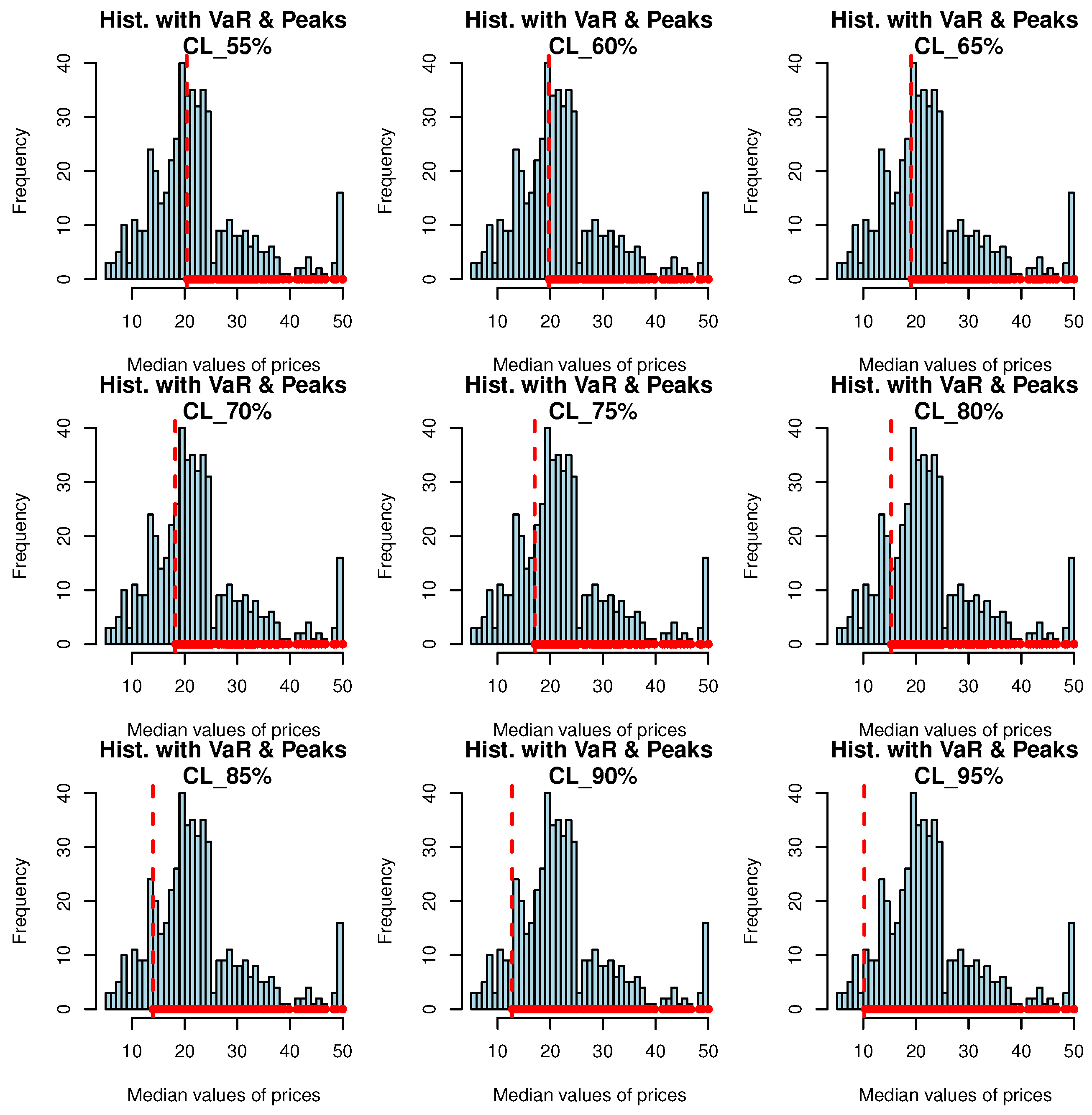
On the other hand, Figure 5 features nine histograms representing the frequency distribution of the median values of Boston house prices across nine CLs. This comparative analysis allows analysts to observe how often certain ranges of failure times occurred during the observed period. Such insights are vital for understanding the behavior of housing prices in extreme conditions, enabling stakeholders to identify trends and anomalies that could impact investment strategies and market stability.
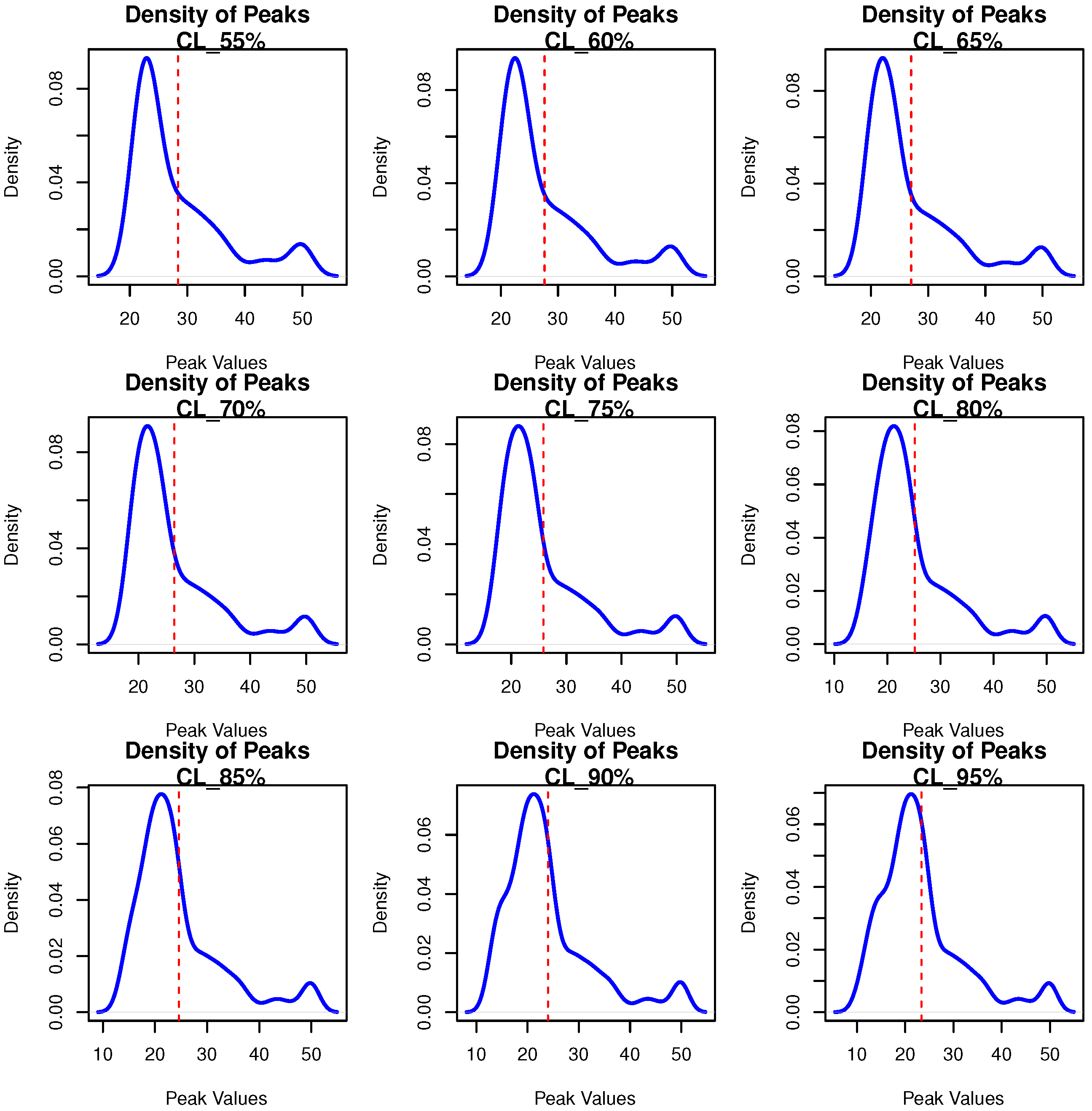
Figure 6 presents a density plot of the peaks at various thresholds, emphasizing the frequency and distribution of significant events (peaks) in the data. This information is crucial for risk assessment, as it enables analysts to gauge the likelihood of extreme fluctuations in the housing market, which can have profound implications for economic stability and investment decisions.
Figure 7 displays the violin plots from the PORT analysis of the median values in the Boston house price data. Each plot illustrates not only the density of the data at different values but also highlights the median and interquartile ranges, offering a thorough understanding of the risk profiles associated with housing investments.
Figure 8 presents the VaR, TVaR, PORT-MOP, and NPORT plots for the median values in the Boston house price data. Figure 5, Figure 6, Figure 7 and Figure 8 support the numerical results in Table 6.
Based on Table 6, we note the following:
  • Financial institutions and investors should integrate these metrics into their risk assessment frameworks to understand potential losses and volatility in the housing market better. By using the VaR and TVaR metrics, stakeholders can develop more robust models for predicting extreme market movements, which can help in formulating strategies to mitigate the risks associated with housing investments.
  • Policymakers should consider implementing measures aimed at stabilizing housing prices, especially when the NPORT values indicate increased occurrences of significant price peaks. Policies such as enhancing support for affordable housing, adjusting interest rates, or providing incentives for first-time homebuyers can help maintain market stability, preventing drastic price fluctuations that could harm the economy.
  • Educational programs should be developed to inform consumers about the risks associated with housing investments and market volatility, particularly in light of rising TVaR and NPORT values. Educating potential buyers about the implications of fluctuating housing prices can help them make informed decisions, reducing the likelihood of panic selling during market downturns, which could exacerbate economic instability.
  • Investors should adopt diversification strategies in their portfolios to mitigate the risks associated with extreme fluctuations in the housing market. By spreading their investments across various asset classes, investors can reduce their exposure to housing market volatility, thereby stabilizing their returns and enhancing their overall portfolio’s resilience.

10. Conclusions

In this article, we introduced a novel family of standard Laplace distributions, expanding the existing statistical framework to capture real-life phenomena better. Throughout this study, we derived several important properties of this new distribution, highlighting its unique characteristics and advantages over traditional models. To demonstrate its practical applicability, we examined the utility of the new distribution using real-life datasets, showcasing how it can be effectively employed in various contexts. Specifically, we utilized a new bimodal skew-logistic model to conduct an in-depth economic risk assessment, leveraging several key metrics, such as value-at-risk (VaR), the peaks over a random threshold value-at-risk (PORT-VaR), tail value-at-risk (TVaR), the mean of order-P (MOP), and the peaks over a random threshold based on the mean of order-P (PORT-MOP). Each of these metrics captures different aspects of the tail behavior, which is crucial for understanding extreme values, particularly in the context of the median house prices in Boston. The PORT-VaR enhances traditional risk evaluations by incorporating randomness into the selection of the thresholds, allowing for a more nuanced understanding of risk exposure. While the VaR and TVaR provide insights into the potential losses at specific confidence levels, TVaR further elucidates significant tail risks by measuring the expected losses beyond the VaR threshold. This distinction is vital for investors and policymakers who need to assess the likelihood and impact of extreme market events. Moreover, the MOP method plays a crucial role in balancing reliability objectives with performance optimizations amid uncertainty. By varying the order of the mean, we can capture a broader range of statistical moments, thereby providing a more comprehensive view of the dataset. This multi-faceted approach is particularly beneficial in economic contexts, where understanding both typical and extreme behaviors is essential for making informed decisions. Equally, this newly introduced model could be extended further in the future by incorporating approaches such as the multi-logistic distribution, and its theoretical development, as well as practical utility, could be examined.

Author Contributions

Conceptualization, J.D., P.J.H. and M.A.; methodology, J.D., P.J.H., M.A. and H.M.Y.; software, J.D., P.J.H., J.D., P.J.H. and M.A.; validation, J.E.C.-R. and H.H.M.; formal analysis, J.D., P.J.H., M.A. and H.M.Y.; investigation, J.D., P.J.H., M.A. and H.M.Y.; resources, J.E.C.-R., M.A. and H.M.Y.; data curation, J.D., P.J.H. and H.M.Y.; writing—original draft preparation, M.A. and H.M.Y.; writing—review and editing, J.E.C.-R. and H.H.M.; visualization, J.D., P.J.H. and H.M.Y.; supervision, J.E.C.-R. and H.H.M.; project administration, M.A.; funding acquisition, J.E.C.-R., M.A. and H.M.Y. All authors have read and agreed to the published version of the manuscript.

Funding

This research received no external funding.

Data Availability Statement

The datasets analyzed during the current study are available from the corresponding author on reasonable request.

Conflicts of Interest

The authors declare that they have no conflicts of interest.

References

  1. Sanyal, S.; Biswas, S.K.; Das, D.; Chakraborty, M.; Purkayastha, B. Boston house price prediction using regression models. In Proceedings of the 2022 2nd International Conference on Intelligent Technologies (CONIT), Hubli, India, 24–26 June 2022; IEEE: Piscataway, NJ, USA, 2022; pp. 1–6. [Google Scholar]
  2. Metwane, M.K.; Maposa, D. Extreme Value Theory Modelling of the Behaviour of Johannesburg Stock Exchange Financial Market Data. Int. J. Financ. Stud. 2023, 11, 130. [Google Scholar] [CrossRef]
  3. Idrovo-Aguirre, B.J.; Contreras-Reyes, J.E. Monetary fiscal contributions to households and pension fund withdrawals during the COVID-19 pandemic: An approximation of their impact on construction labor supply in Chile. Soc. Sci. 2021, 10, 417. [Google Scholar] [CrossRef]
  4. Idrovo-Aguirre, B.J.; Contreras-Reyes, J.E. The response of housing construction to a copper price shock in Chile (2009–2020). Economies 2021, 9, 98. [Google Scholar] [CrossRef]
  5. Idrovo-Aguirre, B.J.; Lozano, F.J.; Contreras-Reyes, J.E. Prosperity or real estate bubble? Exuberance probability index of real housing prices in Chile. Int. J. Financ. Stud. 2021, 9, 51. [Google Scholar] [CrossRef]
  6. Longin, F. The threshold effect in expected utility and mean-variance analysis: Results from a medium-term asset allocation. J. Bank. Financ. 2005, 29, 509–532. [Google Scholar]
  7. Furman, E.; Landsman, Z. Tail variance premium with applications for elliptical portfolio of risks. ASTIN Bull. J. IAA 2006, 36, 433–462. [Google Scholar] [CrossRef]
  8. Landsman, Z. On the tail mean–variance optimal portfolio selection. Insur. Math. Econ. 2010, 46, 547–553. [Google Scholar] [CrossRef]
  9. Taylor, J.W. Estimating value at risk and expected shortfall using expectiles. J. Financ. Econ. 2008, 6, 231–252. [Google Scholar] [CrossRef]
  10. Klugman, S.A.; Panjer, H.H.; Willmot, G.E. Loss Models: From Data to Decisions; John Wiley & Sons: Hoboken, NJ, USA, 2012; Volume 715. [Google Scholar]
  11. Embrechts, P.; Klüppelberg, C.; Mikosch, T. Modelling Extremal Events: For Insurance and Finance; Springer Science & Business Media: Berlin/Heidelberg, Germany, 2013; Volume 33. [Google Scholar]
  12. Kessels, R.; Waldmann, K.H. The relationship between confidence levels and risk measures in quantitative risk analysis. J. Risk Financ. Manag. 2016, 9, 7. [Google Scholar]
  13. Korkmaz, M.C.; Altun, E.; Yousof, H.M.; Afify, A.Z.; Nadarajah, S. The Burr X Pareto Distribution: Properties, Applications and VaR Estimation. J. Risk Financ. Manag. 2018, 11, 1. [Google Scholar] [CrossRef]
  14. Szubzda, F.; Chlebus, M. Comparison of Block Maxima and Peaks Over Threshold Value-at-Risk models for market risk in various economic conditions. Cent. Eur. Econ. J. 2019, 6, 70–85. [Google Scholar] [CrossRef]
  15. de Fondeville, R.; Davison, A.C. Functional peaks-over-threshold analysis. J. R. Stat. Soc. Ser. Stat. Methodol. 2022, 84, 1392–1422. [Google Scholar] [CrossRef]
  16. Alizadeh, M.; Afshari, M.; Ranjbar, V.; Merovci, F.; Yousof, H.M. A novel XGamma extension: Applications and actuarial risk analysis under the reinsurance data. São Paulo J. Math. Sci. 2023, 1, 1–31. [Google Scholar] [CrossRef]
  17. Ibrahim, M.; Emam, W.; Tashkandy, Y.; Ali, M.M.; Yousof, H.M. Bayesian and Non-Bayesian Risk Analysis and Assessment under Left-Skewed Insurance Data and a Novel Compound Reciprocal Rayleigh Extension. Mathematics 2023, 11, 1593. [Google Scholar] [CrossRef]
  18. Alizadeh, M.; Afshari, M.; Contreras-Reyes, J.E.; Mazarei, D.; Yousof, H.M. The Extended Gompertz Model: Applications, Mean of Order P Assessment and Statistical Threshold Risk Analysis Based on Extreme Stresses Data. IEEE Trans. Reliab. 2024. [Google Scholar] [CrossRef]
  19. Elbatal, I.; Diab, L.S.; Ghorbal, A.B.; Yousof, H.M.; Elgarhy, M.; Ali, E.I. A new losses (revenues) probability model with entropy analysis, applications and case studies for value-at-risk modeling and mean of order-P analysis. AIMS Math. 2024, 9, 7169–7211. [Google Scholar] [CrossRef]
  20. Hald, A. Laplace’s theory of inverse probability, 1774–1786. In A History of Parametric Statistical Inference from Bernoulli to Fisher, 1713–1935; Springer: Berlin/Heidelberg, Germany, 2007; pp. 33–46. [Google Scholar]
  21. Aryal, G.R. Study of Laplace and Related Probability Distributions and Their Applications. Ph.D. Thesis, University of Nebraska-Lincoln, Lincoln, NA, USA, 2006. [Google Scholar]
  22. Azzalini, A. A class of distributions which includes the normal ones. Scand. J. Stat. 1985, 12, 171–178. [Google Scholar]
  23. Harandi, S.S.; Alamatsaz, M. Alpha–skew–Laplace distribution. Stat. Probab. Lett. 2013, 83, 774–782. [Google Scholar] [CrossRef]
  24. Shah, S.; Hazarika, P.J.; Chakraborty, S.; Alizadeh, M. The Balakrishnan-Alpha-Beta-Skew-Laplace Distribution: Properties and Applications. Stat. Optim. Inf. Comput. 2023, 11, 755–772. [Google Scholar] [CrossRef]
  25. Chakraborty, S.; Hazarika, P.J.; Ali, M.M. A multimodal Skew Laplace distribution. Pak. J. Stat. 2014, 30, 253–264. [Google Scholar]
  26. Gleaton, J.; Lynch, J. Properties of generalized log-logistic families of lifetime distributions. J. Probab. Stat. Sci. 2006, 4, 51–64. [Google Scholar]
  27. Cordeiro, G.M.; Alizadeh, M.; Ozel, G.; Hosseini, B.; Ortega, E.M.M.; Altun, E. The generalized odd log-logistic family of distributions: Properties, regression models and applications. J. Stat. Comput. Simul. 2017, 87, 908–932. [Google Scholar] [CrossRef]
  28. da Braga, A.S.; Cordeiro, G.M.; Ortega, E.M.; da Cruz, J.N. The odd log-logistic normal distribution: Theory and applications in analysis of experiments. J. Stat. Theory Pract. 2016, 10, 311–335. [Google Scholar] [CrossRef]
  29. Ozel, G.; Altun, E.; Alizadeh, M.; Mozafari, M. The odd log-logistic log-normal distribution with theory and applications. Adv. Data Sci. Adapt. Anal. 2018, 10, 1850009. [Google Scholar] [CrossRef]
  30. da Silva Braga, A.; Cordeiro, G.M.; Ortega, E.M.; Silva, G.O. The odd log-logistic student t distribution: Theory and applications. J. Agric. Biol. Environ. Stat. 2017, 22, 615–639. [Google Scholar] [CrossRef]
  31. Alizadeh, M.; Emadi, M.; Doostparast, M.; Cordeiro, G.M.; Ortega, E.M.; Pescim, R.R. A new family of distributions: The Kumaraswamy odd log-logistic, properties and applications. Hacet. J. Math. Stat. 2015, 44, 1491–1512. [Google Scholar] [CrossRef]
  32. Alizadeh, M.; MirMostafee, S.; Ortega, E.M.; Ramires, T.G.; Cordeiro, G.M. The odd log-logistic logarithmic generated family of distributions with applications in different areas. J. Stat. Distrib. Appl. 2017, 4, 1–25. [Google Scholar] [CrossRef]
  33. Alizadeh, M.; Tahmasebi, S.; Haghbin, H. The exponentiated odd log-logistic family of distributions: Properties and applications. J. Stat. Model. Theory Appl. 2020, 1, 29–52. [Google Scholar]
  34. Afify, A.Z.; Alizadeh, M.; Zayed, M.; Ramires, T.G.; Louzada, F. The odd log-logistic exponentiated Weibull distribution: Regression modeling, properties, and applications. Iran. J. Sci. Technol. Trans. Sci. 2018, 42, 2273–2288. [Google Scholar] [CrossRef]
  35. Alizadeh, M.; K MirMostafaee, S.; Altun, E.; Ozel, G.; Khan Ahmadi, M. The odd log-logistic Marshall-Olkin power Lindley Distribution: Properties and applications. J. Stat. Manag. Syst. 2017, 20, 1065–1093. [Google Scholar] [CrossRef]
  36. Altun, E.; Alizadeh, M.; Ozel, G.; Yousof, H.M. New Odd Log-Logistic Family of Distributions: Properties, Regression Models and Applications. In G Families of Probability Distributions; CRC Press: Boca Raton, FL, USA, 2023; pp. 80–93. [Google Scholar]
  37. Alzaatreh, A.; Lee, C.; Famoye, F. A new method for generating families of continuous distributions. Metron 2013, 71, 63–79. [Google Scholar] [CrossRef]
  38. van der Lecq, M.; van Vuuren, G. Estimating Value at Risk and Expected Shortfall: A Kalman Filter Approach. Int. J. Econ. Financ. Issues 2024, 14, 1–14. [Google Scholar]
  39. Seyfi, S.M.S.; Sharifi, A.; Arian, H. Portfolio Value-at-Risk and Expected Shortfall Using an Efficient Simulation Approach Based on Gaussian Mixture Model. Math. Comput. Simul. 2021, 190, 1056–1079. [Google Scholar] [CrossRef]
  40. Wahed, A.; Ali, M.M. The skew-logistic distribution. J. Statist. Res. 2001, 35, 71–80. [Google Scholar]
  41. Aryal, G.; Nadarajah, S. On the skew Laplace distribution. J. Inf. Optim. Sci. 2005, 26, 205–217. [Google Scholar] [CrossRef]
  42. Charpentier, A.; Flachaire, E.; Ly, A. Econometrics and machine learning. Econ. Stat. 2018, 505, 147–169. [Google Scholar] [CrossRef]
  43. Salem, M.; Emam, W.; Tashkandy, Y.; Ibrahim, M.; Ali, M.M.; Goual, H.; Yousof, H.M. A new Lomax extension: Properties, risk analysis, censored and complete goodness-of-fit validation testing under left-skewed insurance, reliability and medical data. Symmetry 2023, 15, 1356. [Google Scholar] [CrossRef]
  44. Aljadani, A.; Mansour, M.M.; Yousof, H.M. A Novel Model for Finance and Reliability Applications: Theory, Practices and Financial Peaks Over a Random Threshold Value-at-Risk Analysis. Pak. J. Stat. Oper. Res. 2024, 20, 489–515. [Google Scholar] [CrossRef]
  45. Yousof, H.M.; Aljadani, A.; Mansour, M.M.; Abd Elrazik, E.M. A New Pareto Model: Risk Application, Reliability MOOP and PORT Value-at-Risk Analysis. Pak. J. Stat. Oper. Res. 2024, 20, 383–407. [Google Scholar] [CrossRef]
  46. Figueiredo, F.; Gomes, M.I.; Henriques-Rodrigues, L. Value-at-risk estimation and the PORT mean-of-order-p methodology. REVSTAT-Stat. J. 2017, 15, 187–204. [Google Scholar]
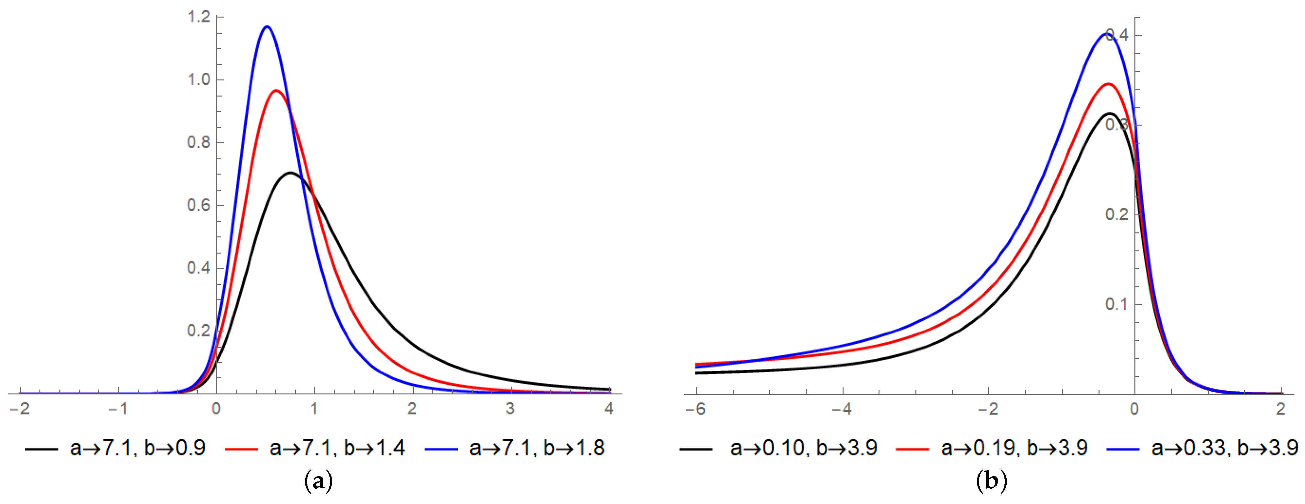
Figure 1. Probability density function (PDF) of NOLLSLa ( a , b ) for several a and b parameters. (a) PDF with large a and small b values to produce a right tail. (b) PDF with small a and large b values to produce a left tail. (c) PDF with small a and b values to concentrate the probability mass around 0. (d) Moderate values of a and b to concentrate the probability mass between 0 and 1.
Mca 30 00004 g001aMca 30 00004 g001b
Figure 2. Cumulative Density Function (CDF) of NOLLSLa ( a , b ) for several a and b parameters related to PDF of Figure 1. (a) CDF in the positive support with large a and small b. (b) CDF in the negative support with small a and large b to produce a left tail. (c) CDF concentrated between 1 and 1 with small a and b values. (d) Moderate values of a and b to concentrate the CDF between 2 and 2.
Mca 30 00004 g002
Figure 3. Plots of observed and expected densities of the Boston (medv) dataset.
Mca 30 00004 g003
Figure 4. The histogram plot, box plot, MOP values P = 1 , 2 , , 15 , and bias versus MSE plot for the the median values in Boston house price data.
Mca 30 00004 g004
Figure 5. PORT-VaR analysis of the median values in the Boston house price data.
Mca 30 00004 g005
Figure 6. Density plot of peaks above the median values in the Boston house price data.
Mca 30 00004 g006
Figure 7. Violin plots for the PORT analysis of the median values in the Boston house price data.
Mca 30 00004 g007
Figure 8. VaR, TVaR, PORT-MOP, and NPORT plots for the median values in the Boston house price data.
Mca 30 00004 g008
Table 1. Simulation results.
μ = 0 , σ = 1
μ σ a b
a b n BiasMSEBiasMSEBiasMSEBiasMSE
20.5100−0.13380.0221−0.87650.6754−0.86980.7692−0.43890.2500
3000.13010.0211−0.62190.51920.81100.51090.31420.2399
500−0.12700.0122−0.61920.5000−0.71320.5021−0.30010.2222
1.51000.11200.31900.31720.63100.23100.08310.33330.3810
3000.10420.3200−0.28100.60090.22100.07220.31990.3511
5000.08100.2910−0.22630.51830.21650.07010.28110.2319
2.51000.28890.3354−0.61100.45190.73100.3317−0.41880.2001
3000.28010.33110.59960.41020.69320.3180−0.37770.0988
5000.26750.31120.49800.37110.61510.2900−0.35100.0888
3.5100−0.19910.0800−0.83110.6107−0.42290.3889−0.51920.2739
300−0.18210.08100.73010.5868−0.39810.33120.49130.2677
5000.18090.07210.70090.47220.37060.22210.46600.2449
4.51000.15040.0329−0.43010.21980.20050.08700.55990.3490
300−0.03410.03010.41600.1998−0.06690.0611−0.69570.2198
5000.02880.0241−0.33000.19970.6660.03990.41410.1765
Table 2. Simulation results.
μ = 0 , σ = 1
μ σ a b
a b n BiasMSEBiasMSEBiasMSEBiasMSE
40.51000.32190.2291−0.41990.31990.49910.32980.31000.4184
3000.21820.21660.39990.29010.47120.3100−0.29900.4000
500−0.20110.19810.38110.2811−0.36140.27660.29000.3911
1.51000.18450.3618−0.28140.41850.2615−0.8621−0.33180.0921
300−0.17190.31720.26170.42100.25100.75140.23410.0715
5000.17100.2001−0.22210.3871−0.25110.61990.23010.0702
2.51000.17650.0861−0.64140.41190.26610.1761−0.04180.1111
3000.15420.05130.61990.39780.26590.1600−0.04030.0833
500−0.15230.04160.58150.36660.25510.15980.38810.0815
3.51000.29910.08810.27710.0661−0.39910.09150.35610.1771
3000.27140.08060.26090.05810.29810.09000.34140.1513
500−0.25990.07710.25100.05060.28810.07160.31100.1333
4.51000.37710.2741−0.28900.34410.16510.24410.14420.0317
300−0.31990.2699−0.27140.32010.17150.22110.13120.0300
5000.30010.25000.26990.31870.17000.18510.09540.0217
Table 3. The MLEs, log-likelihood, AIC, and BIC of models fitted to the Boston (medv) dataset.
Distributions μ σ ab λ logL AIC BIC
N22.5329.188−1840.243684.483692.93
L21.5924.829−1820.073644.133652.58
L a 21.2006.530−1806.263616.523624.97
S N 9.94115.5876.397−1812.393630.783643.45
S L 13.8876.8282.259−1792.763591.523604.20
S L a 19.4006.7400.334−1794.583595.163607.83
O L L S L a 21.2006.7941.034−1806.253618.1503631.189
N O L L S L a 20.1004.2450.9600.539−1789.613587.223604.13
Table 4. LRTs for different hypotheses for the Boston dataset.
        HypothesisLRT Statisticd.f.Critical Values at 5%
H 0 : a = 0 , b = 0 vs. H 1 : a 0 , b 0 33.30025.991
H 0 : b = 0 vs. H 1 : b 0 33.28013.841
Table 5. MOP assessment under P = 1 , 2 , , 25 and the Boston house price data.
P 1 , 2 , 3 , 4 , 5
TMV22.53281
MOP5, 5, 5.2, 5.475, 5.78
MSE307.3993, 307.3993, 300.4262, 290.9688, 280.6565
Bias17.53281, 17.53281, 17.33281, 17.05781, 16.75281
P 6 , 7 , 8 , 9 , 10
MOP5.983333, 6.157143, 6.2875, 6.388889, 6.49
MSE273.88510, 268.16240, 263.91, 260.6261, 257.3716
Bias16.54947, 16.37566, 16.24531, 16.14392, 16.04281
P 11 , 12 , 13 , 14 , 15
MOP6.581818, 6.708333, 6.830769, 6.935714, 7.033333
MSE254.4340, 250.4139, 246.554, 243.2693, 240.2337
Bias15.95099, 15.82447, 15.70204, 15.59709, 15.49947
Table 6. VaR, TVaR, and PORT-MOP for the Boston house price data.
CLs↓VaRTVaR T h PORT-MOPNPORTMin.; 1st Qu.; Med; ExV; 3rd Qu.; Max.
55%22.030.1228.095027620.50 22.60 24.70 28.37 31.77 50.00
60%22.730.9228.155030319.80 22.00 24.20 27.64 31.05 50.00
65%23.332.1238.758332719.20 21.45 23.80 27.04 30.10 50.00
70%24.233.3249.158635318.30 20.80 23.30 26.42 29.60 50.00
75%25.035.32510.259037917.10 20.25 23.10 25.82 28.70 50.00
80%28.237.2288.961440515.30 19.70 22.70 25.20 28.20 50.00
85%31.039.7318.651343014.00 19.30 22.30 24.58 27.50 50.00
90%34.843.1318.331445512.80 18.70 22.00 23.97 26.65 50.00
95%43.448.5435.053847910.40 17.85 21.70 23.35 26.30 50.00
Disclaimer/Publisher’s Note: The statements, opinions and data contained in all publications are solely those of the individual author(s) and contributor(s) and not of MDPI and/or the editor(s). MDPI and/or the editor(s) disclaim responsibility for any injury to people or property resulting from any ideas, methods, instructions or products referred to in the content.