Symbolic Regression for the Determination of Joint Roughness Coefficient

Abstract

In this study, a novel symbolic regression-based empirical equation has been developed to compute the joint roughness coefficient (JRC) value based on the statistical parameters of rock joints. The symbolic regression was adopted to map the nonlinear function, which represents the relation between the JRC and statistical parameters of the rock joint, based on the collected rock joint dataset. It is not necessary to presume the mathematical function form of the empirical equation, which is used to fit the rock joint data while using symbolic regression. The collected rock joint samples from the literature were used to investigate and illustrate the developed symbolic regression-based empirical equation. The performance of the developed empirical equation was compared to the traditional empirical equation. The results show that the generalization performance of the developed empirical equation is better than the traditional empirical equation. They proved that the symbolic regression-based empirical equation characterized the roughness property of rock joints well and that symbolic regression could be used to capture the complex and nonlinear relationship between JRC and the statistical parameters of rock joints. The developed symbolic regression-based empirical equation provides a scientific and excellent tool to estimate the JRC value of rock joints.

1. Introduction

Joint roughness is critical to the strength, deformation, and failure mechanism of the rock mass. The joint roughness coefficient (JRC) is commonly used to describe the roughness property of rock joints and estimate the peak shear strength of rock joints in rock mass engineering [1]. In the 1970s, Barton and Choubey first proposed a visual comparison method to determine the JRC value based on the ten standard rock joint profiles [2]. Then, this method was adopted by the International Society of Rock Mechanics (ISRM) Commission on Test Methods [3]. However, the obtained JRC value is variable and uncertain, based on the user judgment due to the subjectivity of visual comparison. In order to characterize the joint property reasonably and overcome the abovementioned limitation, various statistical parameters of the joint profile, such as the arithmetical mean deviation roughness index of the profile (R_a), the root mean square roughness index of the profile (R_q), and the mean square value roughness index (M_s), were defined to describe the rock joint profile [4].

Table 1. List of symbols for joint.

Symbol	Definition
JRC	joint roughness coefficient
Z2	first deviation of the profile
SF	structure–function
Ra	arithmetical mean deviation roughness index of the profile
Rq	root mean square roughness index of the profile
Ms	mean square value roughness index
Rp	roughness profile index
δ	profile elongation index
σi	standard deviation of the angle
λ	ultimate slope of profile

lists the definition of some statistical parameters of rock joints. However, it is still not easy to characterize and quantify the roughness property using JRC due to the complexity and uncertainty of rock joints. Thus, it is a challenging task to obtain a consistent JRC value in practical rock engineering.

In the last decades, many methods have been proposed to estimate the JRC value of rock joints for practical rock engineering [4,5]. Regression analysis is a commonly used way to establish the empirical equation based on the statistical parameters of rock joint profiles. Tse and Cruden (1979) established the regression equation of JRC based on the mean root square of the first deviation of the profile (Z₂) and the structure–function (SF) [6]. Wang (1982) developed an empirical equation of JRC based on the R, defined as the difference between the actual and the projected length of a profile [7]. The roughness profile index (R_p) is the ratio of the true length of a fracture surface trace to its projected length in the fracture plane [8]. Maerz et al. (1990) established the JRC empirical equation of JRC based on Rp and the profile elongation index (δ) [9]. The standard deviation of the angle (σ_i) was defined to describe the roughness of rock joints and used to estimate the JRC [10]. Barton and de Quadros (1997) adopted the ultimate slope of the profile (λ) to estimate the JRC value [11]. Yang et al. (2001) reconstructed the ten standard profiles and improved the empirical equation of JRC based on Z₂ and SF using the Fourier transform [12]. Li and Zhang (2015) reviewed the JRC empirical equation and derived the corresponding JRC empirical equation [13]. The abovementioned empirical equations are obtained using regression analysis based on a single statistical parameter. These methods ignore the interaction of the statistical parameters and need to be revised to characterize the JRC of the rock joints comprehensively [14]. Gao and Wong (2013) established the JRC empirical equation using Z₂ and the normalized amplitude, a newly defined parameter of rock joints [15]. The relative waviness and elongation of the rock joint were also defined and utilized to establish the JRC empirical equation [16]. The regression equations are often established based on the ten standard joint profiles using the regression method. Thus, these empirical equations were good and can only characterize the roughness property of the ten standard rock joint profiles. Furthermore, these equations have poor performance for generalization. They struggle to predict the JRC of the new unknown rock joints in practical rock engineering. Some researchers introduced the fractal dimension, a tool for describing the degree of variation in a curve, a surface, and a volume, to characterize the rock joint profile by establishing the JRC empirical equation. Various empirical equations were proposed to estimate the JRC value based on the fractal dimension [17,18,19,20,21,22]. However, these are difficult to apply in practical rock engineering due to the uncertainty of fractal dimension determination methods. The traditional empirical equation method has encountered great difficulties in characterizing and quantifying JRC based on the statistical parameters of the joint profile.

With the development of artificial intelligence and machine learning, various intelligent methods, such as artificial neural networks, support vector machines, or symbolic regression, have been widely used in civil engineering [23,24,25,26,27,28,29,30,31]. A support vector machine model was proposed to determine the JRC value based on the eight statistical parameters of rock joints [32]. Fathipour-Azar (2021) established various machine learning models, such as the Gaussian process, K-star, random forest, or extreme gradient boosting, to determine the JRC value and compared their performance with the traditional empirical equation [33]. Miao et al. (2021) utilized a boosting decision tree model to determine the JRC of the rock joint profile based on its statistical parameters [34]. A deep learning model with a time–frequency spectrogram was proposed to determine the JRC of rock joints [35]. Machine learning provides an excellent tool for capturing complex and nonlinear engineering system relationships. However, machine learning methods have disadvantages, such as “black-box” characteristics, overfitting, and trapping local minimum. It is not easy to interpret and characterize the mechanism and behavior of the physical model in explicit equations. Thus, this hinders both interpretations of the results and their application in the practical engineering system [36].

Symbolic regression is a machine learning method that can obtain a closed-form equation based on the input features [37]. Meanwhile, symbolic regression can derive a valuable equation from approximating the complex and nonlinear function of an engineering system [38]. The closed-form equation is often obtained automatically based on the samples [39]. It has been successfully applied in civil engineering [24]. Compared with other machine learning methods [40], the main advantage of symbolic regression is that the final model is expressed in a closed-form mathematical equation [41] and can mine the physical mechanism behind the data and establish the closed-form equation for presenting the complex and nonlinear relationship between the JRC value of rock joint and their roughness property. Symbolic regression provides an excellent way to capture the complex relationship between the JRC of rock joints and their roughness property.

Symbolic regression is a flexible and data-driven regression method that discovers the explicit mathematical equation to capture the physical mechanism and behavior of an engineering system [42]. In this study, symbolic regression was used to capture the roughness of the rock joint and compute the JRC value based on the statistical parameters of the joint profile. The remainder of this paper is organized as follows. Firstly, the joint roughness coefficient and the traditional empirical equation are introduced in detail in Section 2. Secondly, the idea, theory, framework, and procedure of the symbolic regression-based JRC determination model are presented briefly in Section 3. Then, the proposed empirical equation is applied to the collected rock joint, and their performances and comparison with the other empirical equation are demonstrated and discussed in Section 4. Finally, some conclusions are presented in Section 5.

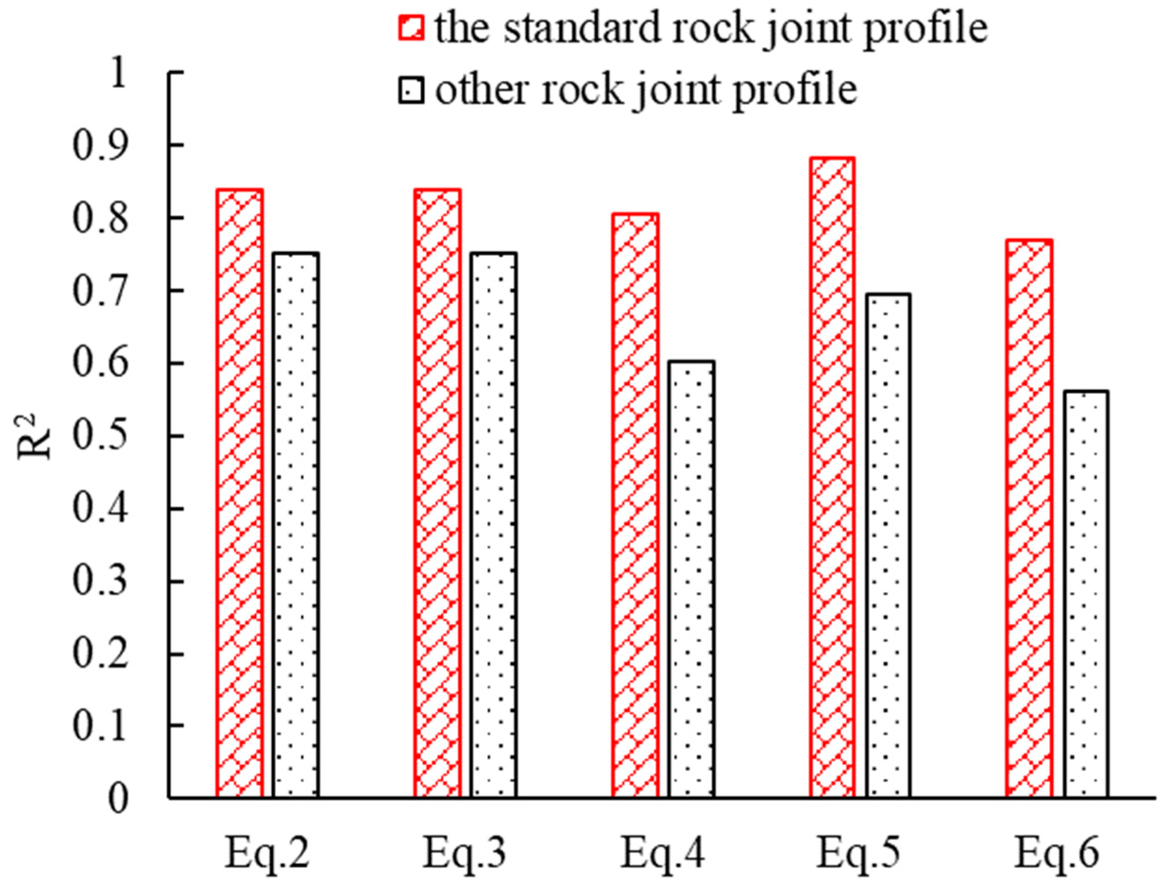
2. Review of the JRC Empirical Equation

JRC value is critical to evaluate the strength and stability of the joint rock mass in practical rock engineering. Barton and Choubey (1977) estimated the value of JRC by visibly comparing it with the ten standard rock joint profiles. However, Barton’s method may provide different JRC values for different users and engineers due to the subjectivity of judgment on which standard joint profile fits the best. In order to avoid the subjectivity of Barton’s method, various empirical equations have been developed to estimate the JRC based on the statistical parameters using the regression method. Generally, the empirical equation was established to quantify objectively the joint roughness property based on the various statistical parameters of rock joints using regression technology. The commonly used statistical parameters of rock joints include Z₂, SF, R_p, δ, λ, R_q, R_a, etc. The general form of the regression equation is as follows.

$$JRC=a+bf(C_J)$$

(1)

where a and b are the unknown regression coefficients that depend on the statistical parameters of the rock joint profile. C_J is the statistical parameters of the rock joint profile, such as Z₂, SF, λ, R_p, δ, R_q, and R_a. $f(\cdot )$ is the specific unknown function, such as linear function, logarithmic function ($\log (\cdot )$), square root function ($\sqrt{ }$), or trigonometric function ($\tan (\cdot )$), which will be determined based on the regression method.

Various empirical equations have been obtained by presuming the different unknown functions $f(\cdot )$ and determining the unknown regression coefficients a and b based on different statistical parameters C_J of the rock joint using the regression method. The traditional empirical equations heavily depend on presuming the unknown function $f(\cdot )$ and the statistical parameters C_J of the rock joint. Tse and Cruden (1979) proposed the following empirical equations (Equations (2)–(6)) using the Z₂, SF, R_p, R_q, and M_s. The correlation coefficients of Equations (2) and (3) are both greater than 0.84 for the ten standard rock joint profiles, which are the samples for the regression analysis. The correlation coefficients of Equations (4)–(6) are all lower than the result of Equations (2) and (3). However, the correlation coefficients of Equations (4)–(6) are greater than 0.69. This shows that the empirical equation has a good performance. However, the correlation coefficient of the empirical equation is about 0.7130 for the other 12 joint profiles, which is different from the standard joint profile (Figure 1). This shows that the empirical equation has poor generalization performance. In other words, it is not feasible to estimate the JRC using the empirical equations (Equations (2)–(6)) for the other rock joint profiles in practical rock engineering. These empirical equations are limited due to their poor generalization performance, which hinders their application in practical engineering.

$$JRC=32.2+32.47\log (Z_2)$$

(2)

$$JRC=37.28+16.58\log (SF)$$

(3)

$$JRC=558.68\sqrt{R_p}-557.13$$

(4)

$$JRC=2.76+78.87R_a$$

(5)

$$JRC=5.43+293.97M_s$$

(6)

3. Materials and Methods

Various empirical equations have been developed to estimate the JRC based on the statistical parameters of the rock joint using regression analysis. These empirical equations perform well for the rock joint used for regression analysis. However, the performance of empirical equations is less than satisfactory for the rock joint that is not included in the regression samples. This limits and hinders the application of empirical equations in practical rock engineering. In this study, symbolic regression was adopted to search the JRC empirical equation based on various statistical parameters of the rock joint. The determined empirical equation has a good performance and excellent generalization performance, which extends its application in practical rock engineering. Symbolic regression provides an excellent, feasible, and helpful tool to characterize the roughness property and estimate the JRC value for rock joints.

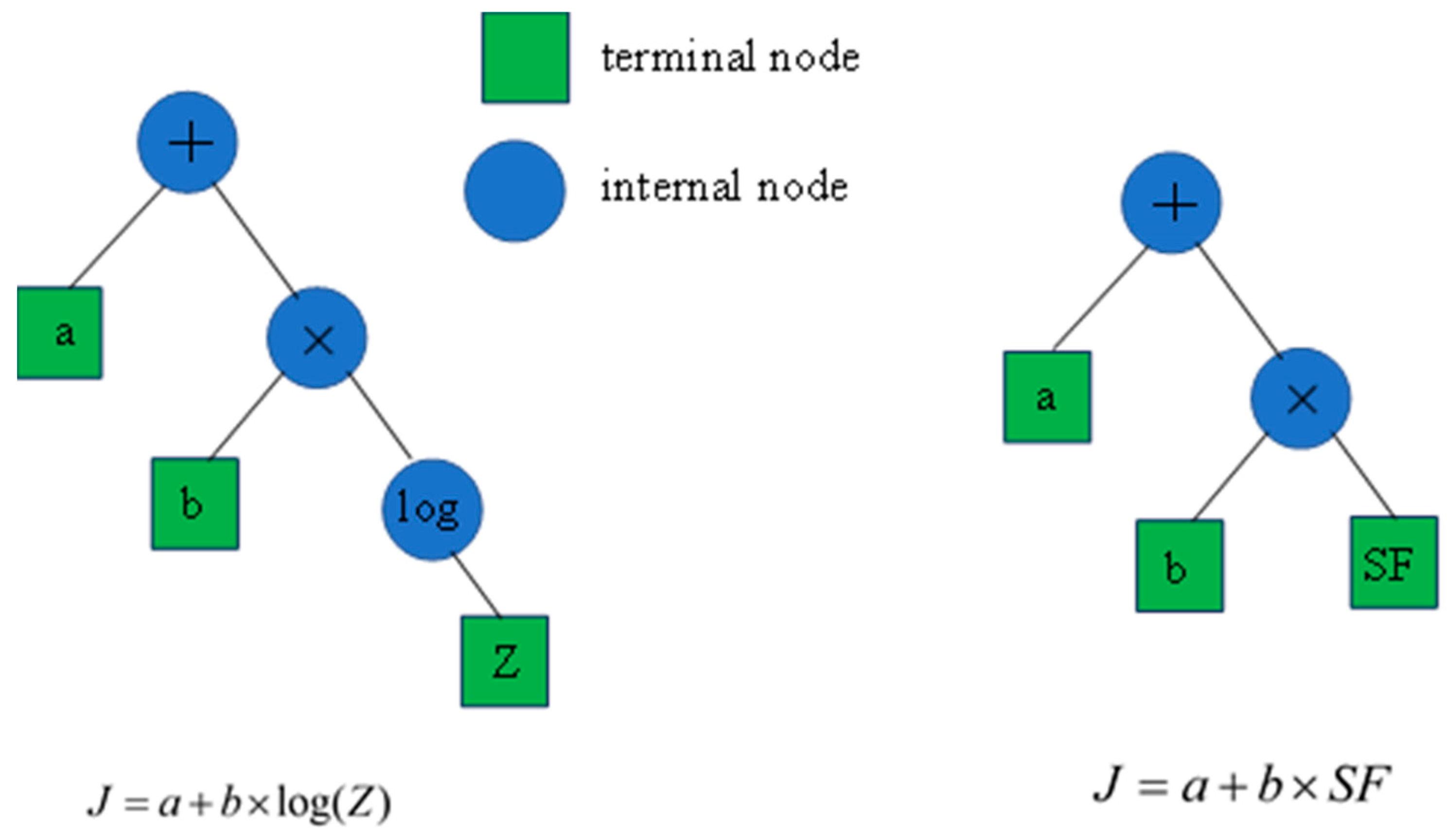
3.1. Symbolic Regression

Symbolic regression is a kind of machine learning approach to discovering a suitable mathematical function to characterize the relationship between dependent variables in engineering systems based on data [43,44]. Compared with the traditional regression method, symbolic regression does not need a priori assumptions on the specific form of the function [24]. A mathematical expression space in symbolic regression contains mathematical operators, state variables, constants, and analytic functions. Symbolic regression can be searched in the mathematical expression space to discover a mathematical equation that fits the relation of the variables based on data. Any equation can be expressed as a binary tree in symbolic regression. The binary tree structure comprises the terminal and internal nodes. The terminal node represents the constant and variable, and the internal node represents the function and operation symbols in symbolic regression. Figure 2 shows the binary tree representation equation in symbolic regression.

Combining simpler trees (simple mathematical equations) can automatically generate more complex trees (complex mathematical equations). Optimization technology is commonly utilized to combine simpler trees to generate complex trees to approximate the response of the engineering system. In optimization technology, the new equation (trees) is selected based on the fitness function; the higher the fitness, the higher the probability that the new expression (trees) is selected. Genetic programming is an evolutionary algorithm inspired by Darwinian principles of natural selection and is commonly used in symbolic regression as the optimization technology. Genetic programming evolves equation trees to generate mathematical equations that provide optimal fitness values. The initial population is randomly generated based on the defined function according to the genetic programming. Individuals are selected according to their fitness. New individuals will be generated and evolve through one-point crossover and single-point mutation (Figure 3). In this study, genetic programming was adopted to generate a random population of tree-structured symbolic expressions by combining several functions, such as addition (+), multiplication (×), subtraction (−), division (÷), square root, reciprocal, and power, with input parameters and random constants. Depending on the problem’s needs, the function can be added and customized.

This study employed a systematic approach of genetic programming-based symbolic regression to discover the JRC estimation equation. The genetic programming procedure, a step-by-step process of initialization, evaluation, selection, crossover, and mutation, is defined as one cycle or one generation of the analysis. This process is repeated until the maximum number of cycles is finished or the optimal equation is obtained. The procedure of the genetic programming-based symbolic regression is briefly described as follows.

• Step 1: Determine the maximum cycles, population size, probability of crossover and mutation, etc.
• Step 2: Set the mathematical expression space for symbolic regression.
• Step 3: Generate the initialized population for genetic programming randomly.
• Step 4: Evaluate each individual in the population and determine their fitness value.
• Step 5: Generate the new population based on the genetic operator, such as selection, crossover, or mutation.
• Step 6: Meet the stop criterion and obtain and output the final JRC equation. Otherwise, repeat steps 4 and 5.

3.2. The JRC Presentation Based on Symbolic Regression

The roughness property has to do with the morphological characteristics of the rock joint, and the JRC reflects the morphological feature of the rock joint. Due to the complex and nonlinear relationship between JRC and the joint morphological features, it is difficult to capture using a simple empirical equation. Symbolic regression can derive the complex relation of the JRC and their influence factor. In this study, symbolic regression was employed to construct the complex function mapping between JRC and the statistical parameters of the rock joint and characterize the roughness property of the rock joint. The symbolic regression model of JRC SR(X, Y) can be presented as follows.

$$SR\left(X\right):R^N\to R$$

(7)

JRC = SR (X)

(8)

where X = (x₁, x₂, …, x_N), and x_i(i = 1, 2, …, N) denotes the statistical parameters of the rock joint, such as Z₂, SF, R_a, λ, or δ. JRC denotes the joint roughness coefficient of the rock joint.

To establish SR(X), some known rock joints (training samples) are needed. This study collected the necessary samples from the literature. The statistical parameters, such as Z₂, SF, R_a, λ, or δ, can be obtained based on their definition based on the rock joint profile. Then, the JRC value can be obtained based on the test and the characterizations of the joint profile. This study used SR to map the complex and nonlinear function relation between the JRC and the statistical parameters of the rock joint profile.

3.3. Procedure of Symbolic Regression-Based JRC Empirical Equation

This study developed a symbolic regression-based JRC determination model based on SR and the rock joint samples collected from the literature. The SR was employed to characterize the relationship between the JRC and the statistical parameters of the rock joint profile. The brief procedure of the symbolic regression-based JRC determination model is presented below. Figure 4 shows the flowchart of the symbolic regression-based JRC determination model.

• Step 1: Collect the rock joint samples, determine JRC by test, and compute the statistical parameters.
• Step 2: Construct the training samples based on the JRC and the corresponding statistical parameters of the rock joint.
• Step 3: Select and set the parameters and operator of the symbolic regression algorithm.
• Step 4: Call the symbolic regression algorithm based on the abovementioned training samples.
• Step 5: Generate the empirical equation based on the symbolic regression.
• Step 6: Estimate the JRC value for the new unknown rock joint based on the generated empirical equation.

4. Results

This study revisited 112 rock joint datasets collected from the literature [13,32]. They were utilized to demonstrate the developed symbolic regression-based JRC determination model. The statistical parameters of the rock joint were computed, and symbolic regression was utilized to determine the empirical equation. The performance of the developed model was illustrated and discussed based on the unknown rock joint, which was not included in the training samples.

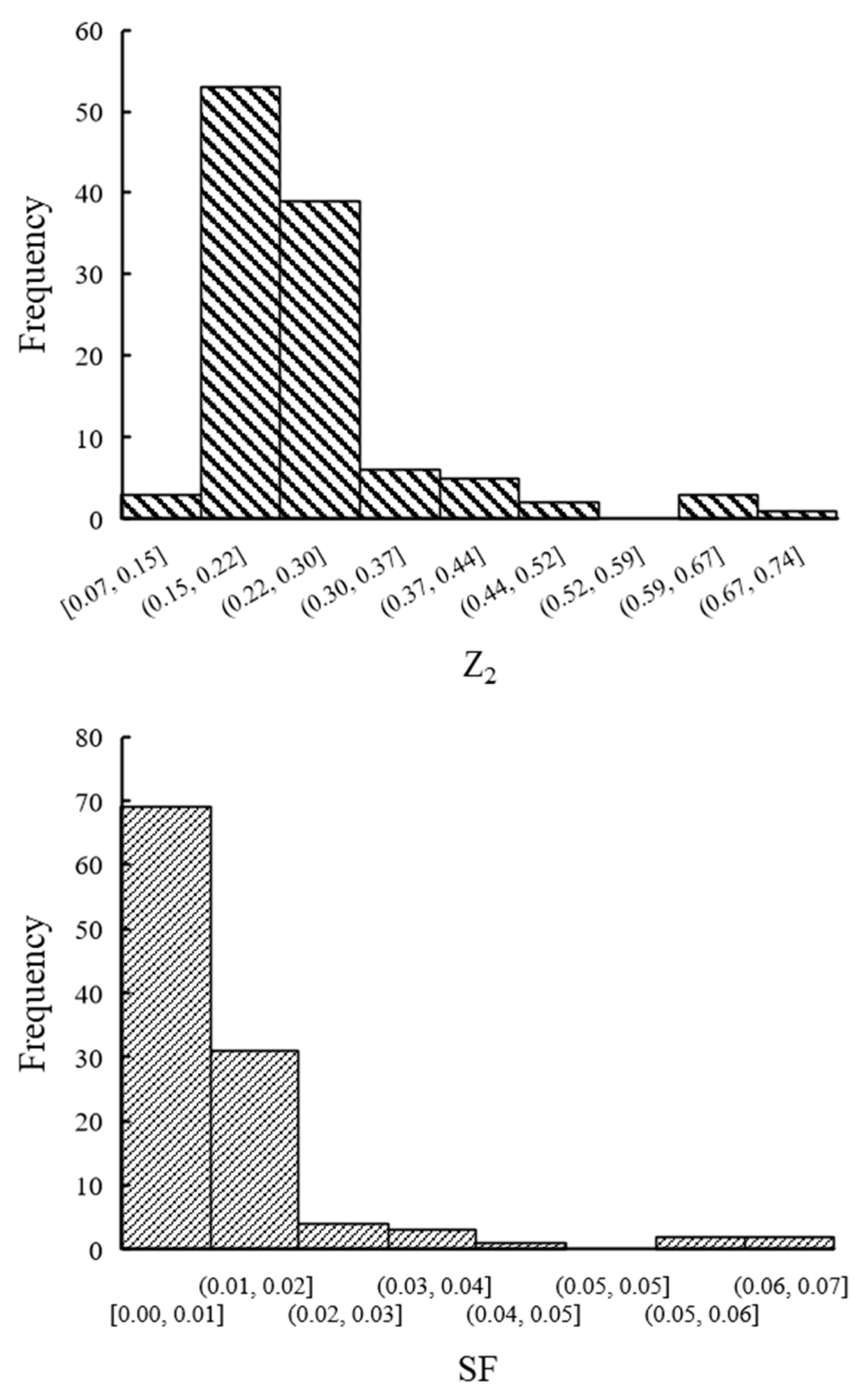
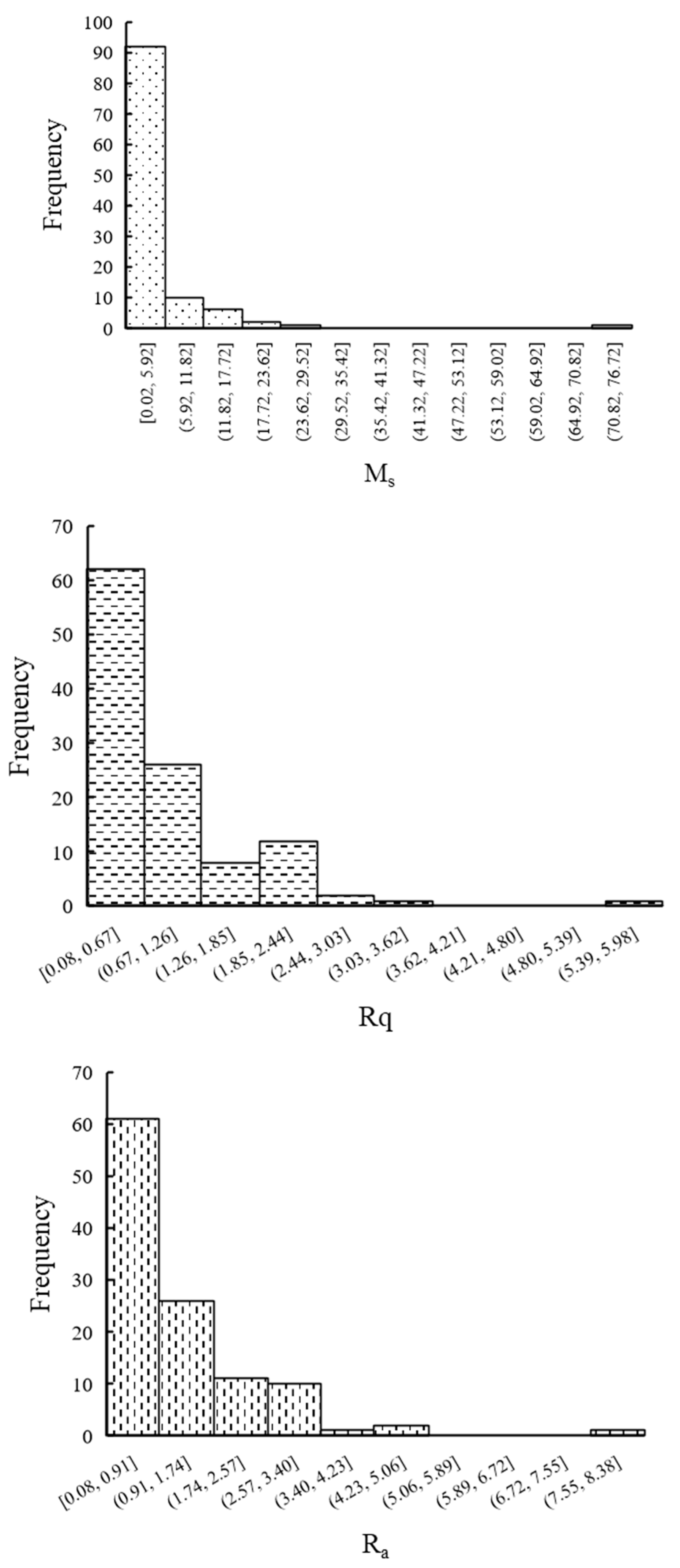
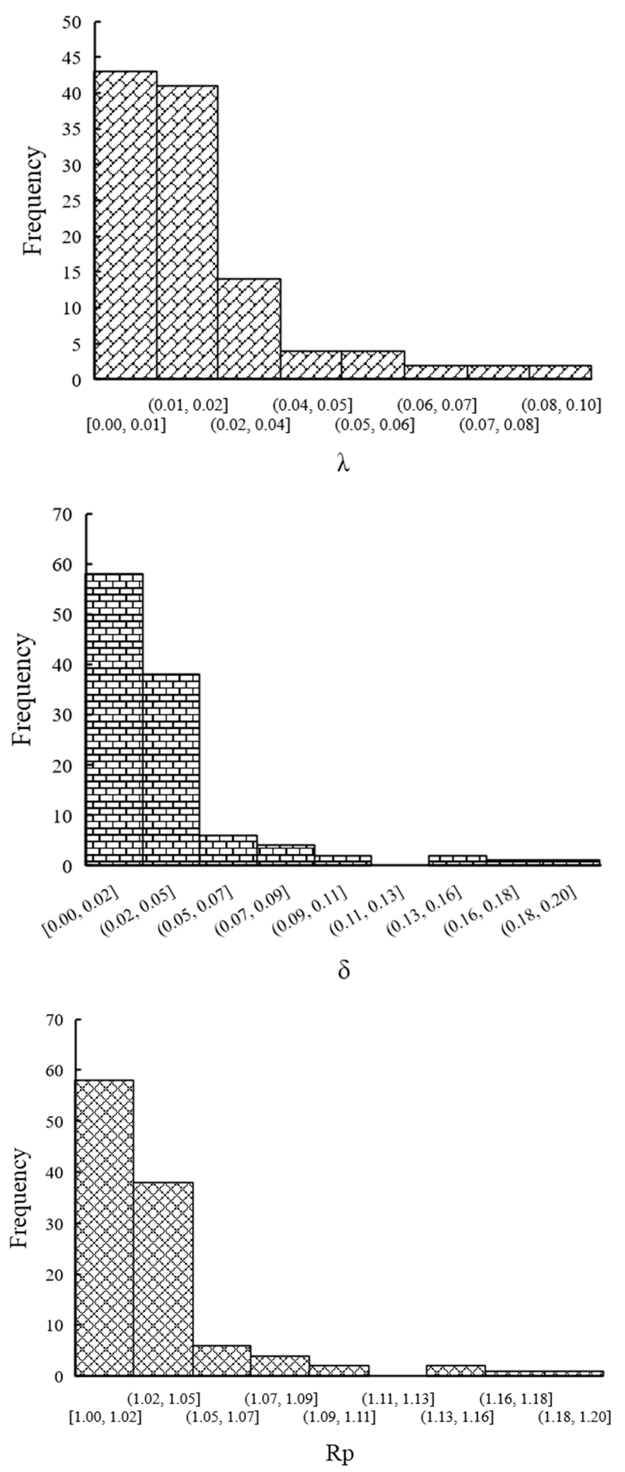
4.1. Dataset of the Rock Joint

The statistical parameters of each rock joint were computed for the 112 rock joints according to their definition. Figure 5 shows the statistical properties of corresponding parameters for the collected rock joints. The distribution of statistical parameters varies greatly, which poses a challenge to scientifically and reasonably determining joint characteristics. Detailed information on joint data can be found in the literature [13,32]. Each rock joint, regarded as symbolic regression input, includes eight statistical parameters (Z₂, SF, R_p, δ, λ, R_q, R_a, and M_s). The corresponding JRC, the output of symbolic regression, was determined based on the statistical parameters of the rock joint. The training samples comprised the statistical parameters and corresponding JRC value of the rock joint for symbolic regression. In order to investigate the performance of symbolic regression, the 112 rock joint profiles were divided into two groups. One group included 100 rock joint profiles. The other group had 12 rock joint profiles that were utilized to investigate the performance.

The correlation between the statistical parameters of rock joints and their JRC was investigated based on the collected samples. Figure 6 shows their correlation coefficient heatmaps. The results show that all correlation coefficients are greater than 0.75. We conclude that the statistical parameters of the joint have a strong correlation and are not independent. This is consistent with their definition, which is determined by the size of the horizontal x and altitude y of the joint profile. In other words, each statistical parameter only characterizes one local feature of the rock joint and cannot fully characterize its features. It further proved that the traditional empirical equation has poor generalization performance. Additionally, Figure 6 shows that the correlation of Z₂, SF, and JRC is strong. This proves that the empirical equation with Z₂ and SF has a higher correlation coefficient (R²). Meanwhile, the correlation of R_a, R_q, M_s, and JRC is poor. The empirical equation with R_a, R_q, and M_s has a lower correlation coefficient (R²). We conclude that the empirical equation is reasonable, though it cannot fully represent the roughness of rock joints. In order to scientifically and reasonably characterize the roughness property of rock joints, the empirical equation should consider the multiple statistical parameters of rock joints.

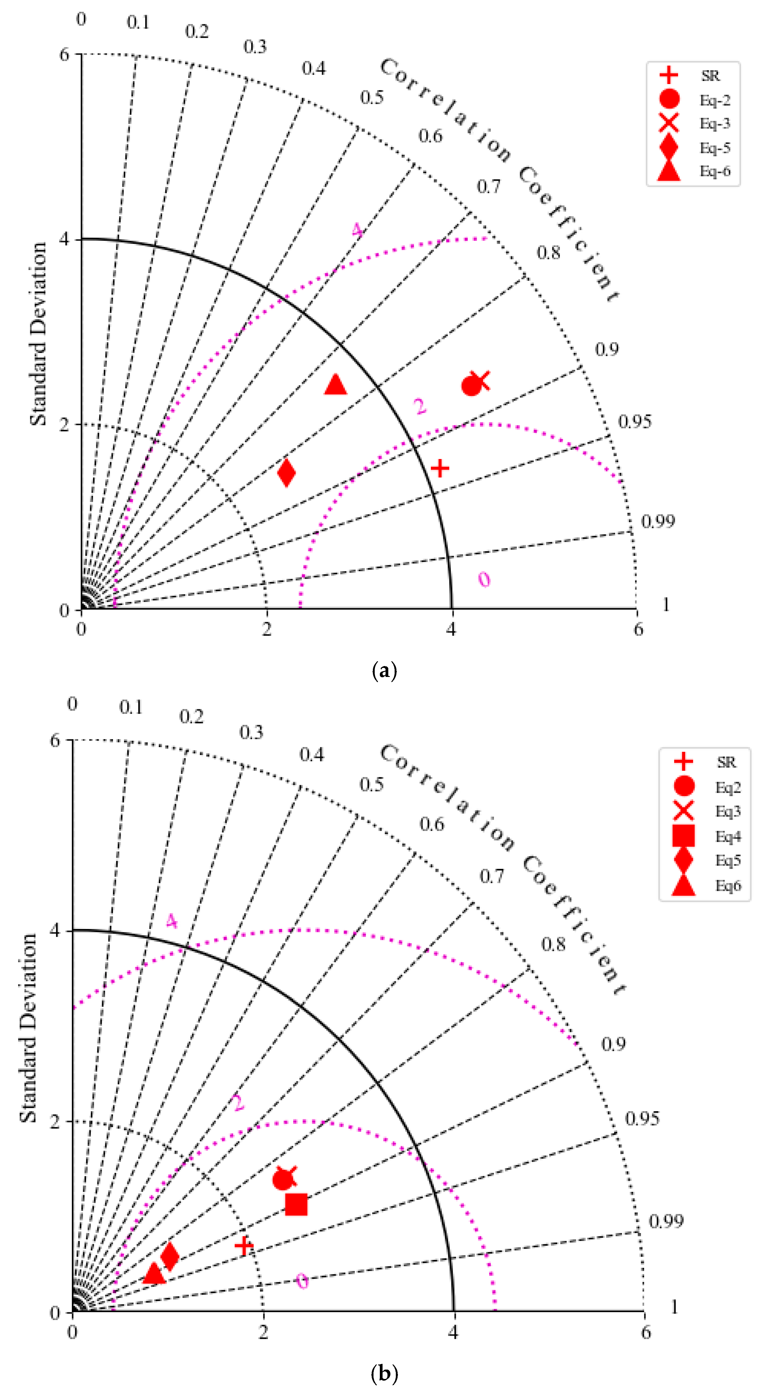
4.2. Determination of JRC Using Symbolic Regression

Symbolic regression was adopted to construct the empirical equation for estimating the JRC based on the statistical parameters of the collected rock joints. A total of 100 rock joint profiles were the training samples to construct the JRC determination equation. According to the procedure of symbolic regression, a symbolic regression model was generated in Figure 7. Based on the symbolic regression model, the empirical equation (Equation (9)) was obtained by symbolic regression.

$$JRC=\left({\displaystyle \frac{Z_2}{0.113}}-0.013{\displaystyle \frac{Z_2}{SF}}\right)\left({\displaystyle \frac{Z_2}{SF}}\sqrt{\lambda }+0.476\right)$$

(9)

The JRC value was determined using the empirical equation obtained for rock joints. Figure 8 compares the actual JRC and the predicted JRC by symbolic regression. It shows that the predicted JRC by symbolic regression is in excellent agreement with the actual JRC for the training and testing of rock joints. The correlation coefficients are 0.89, 0.88, and 0.87 for the training rock joint, ten standard rock joints, and the testing rock joint. This proved that the empirical equation obtained by symbolic regression characterizes the complex relationship between the roughness property and the statistical parameters of rock joints well. Moreover, the obtained empirical equation has a good generalization performance. Symbolic regression can be used to estimate the JRC value and provides an excellent way to characterize the roughness property based on the statistical parameters of rock joints.

To further demonstrate the performance of the obtained equation, it was compared with the traditional empirical equation (Equations (2)–(6)), which includes various statistical parameters of rock joints and has a higher correlation coefficient. The Taylor diagram (Figure 9) shows the performance comparison between the obtained equation by symbolic regression and the traditional empirical equations for the training and testing of the rock joint. In Figure 9a, the correlation coefficient obtained by symbolic regression is higher than that obtained by the traditional empirical equations, and the standard deviation and root-mean-square error are lower than those obtained by the traditional empirical equations for training samples. In Figure 9b, although the standard deviation is higher than the traditional empirical equations, the root-mean-square error is lower than that obtained by the traditional empirical equations, and the correlation coefficient is also higher than the traditional empirical equations for the testing samples. The empirical equation obtained by symbolic regression performed excellently. This also proved that symbolic regression has more advantages than traditional regression. Symbolic regression reveals the roughness mechanism and law based on the statistical parameters of the rock joint. Figure 10 shows the comparison between JRC determined by the obtained equation by symbolic regression and the empirical equations. This proved that the determined JRC by symbolic regression was closer to the actual JRC than the empirical equations using the regression analysis. The results show that symbolic regression captures the roughness property based on the statistical parameters of the rock joint.

5. Discussion

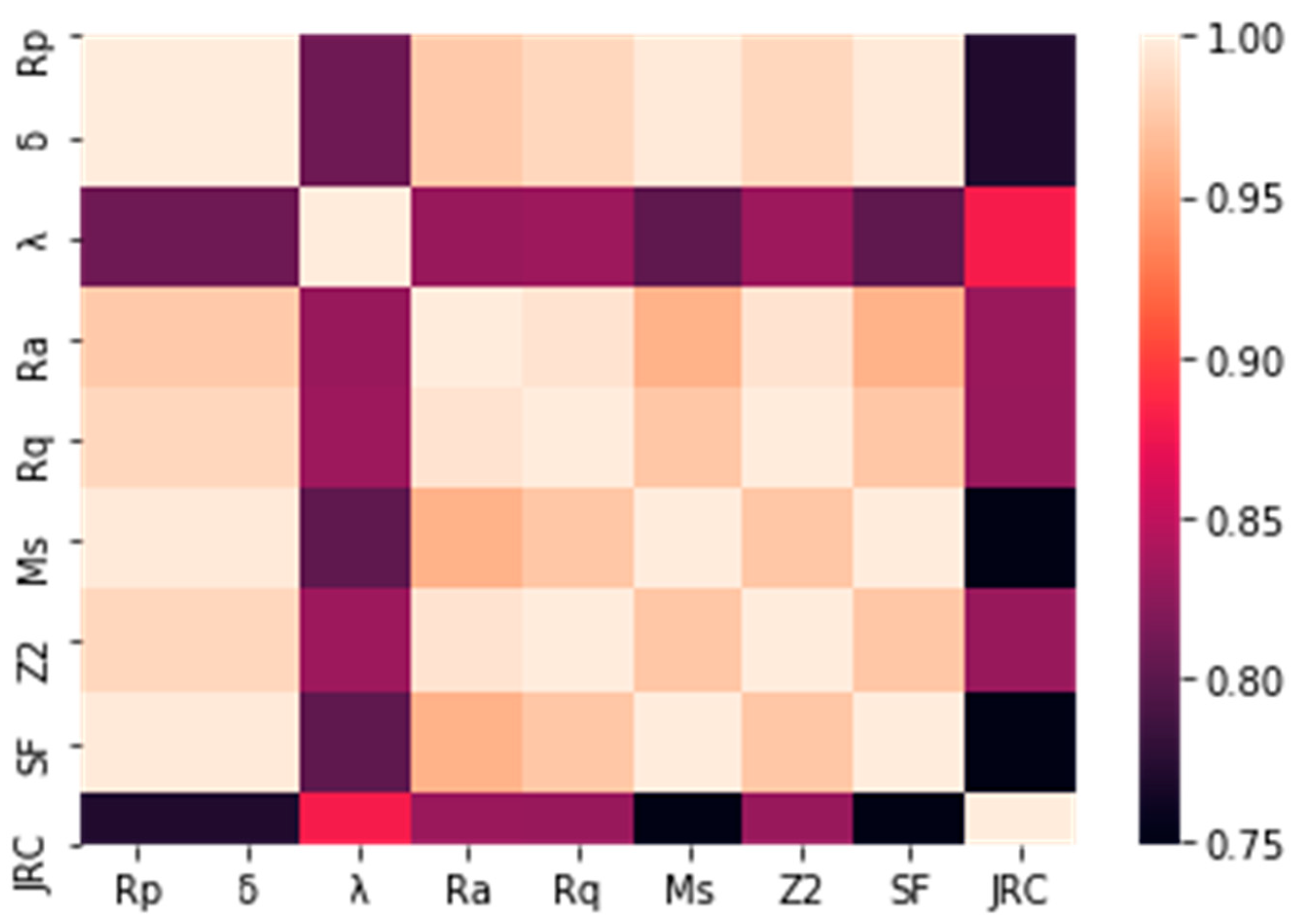
5.1. The Relationship Between JRC and the Statistical Parameters of the Rock Joint

According to the traditional empirical equation, the JRC value can be determined based on the statistical parameters of rock joints. However, the generalization performance of the traditional empirical equation is poor due to the complex roughness property. It is difficult to determine the JRC value based on the single statistical parameters of rock joints. Figure 11 shows the relationship between Z₂, SF, and JRC. Their relationship is complex and nonlinear. Meanwhile, JRC is also impacted by the interaction between the statistical parameters. This further proved that the traditional empirical equation could not characterize the roughness well using the single statistical parameters of rock joints. Symbolic regression can capture the interaction between the statistical parameters.

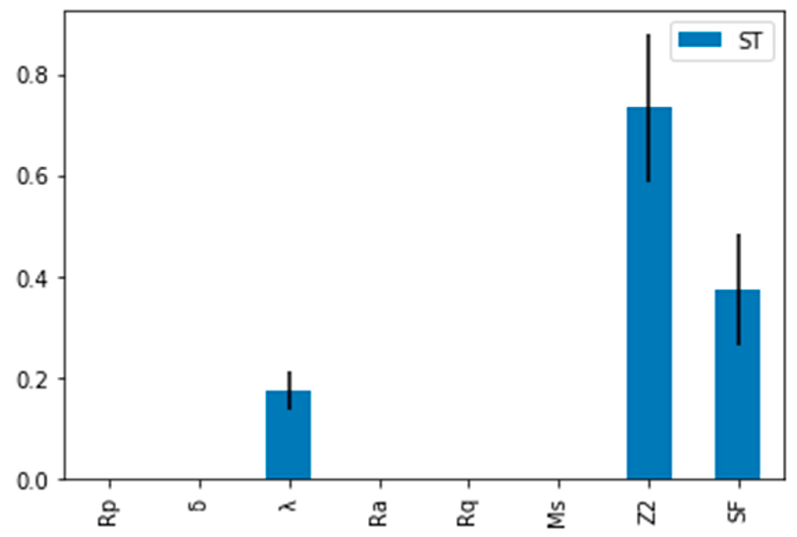
5.2. Sensitivity Analysis

In this study, the eight statistical parameters of rock joints were selected to establish the JRC determination equation using symbolic regression. A sensitivity analysis was adopted to evaluate the impact of statistical parameters on the JRC value based on the obtained equation. Figure 12 shows the total sensitivity of each statistical parameter of the rock joint. We can see that Z₂ has the most significant impact on the JRC and can characterize the roughness property of rock joints. Next, SF is critical to the determination of JRC. This further proved that Z₂ and SF are essential and sensitive to the roughness property of rock joints. Moreover, the empirical equation, which includes Z₂ and SF, performs better than the equation with other statistical parameters of rock joints. Symbolic regression can characterize the roughness mechanism using the collected rock joint data. Additionally, the sample size is critical to symbolic regression. With the increase in the number of samples, the performance of the developed model will be enhanced further.

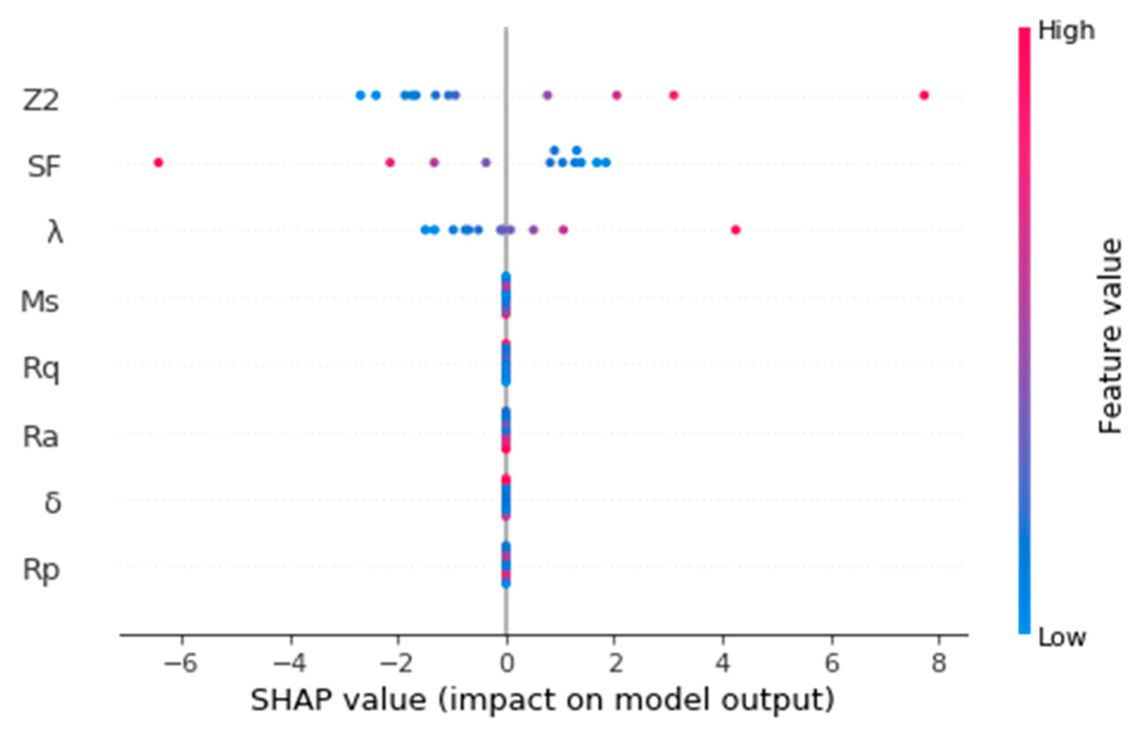
5.3. Feature Analysis of Symbolic Regression Model for JRC

This study investigates the importance of the statistical parameters of rock joints using the SHAP value. Figure 13 shows the importance of the JRC of each statistical parameter of the rock joint. Z₂, SF, and λ are the essential features of rock joints, which reflect the toughness of the joint. Moreover, this result agrees with the correlation analysis (Figure 6) and sensitivity analysis (Figure 12). Figure 14 shows the influences of statistical parameter variation on the JRC. We can see that the increase of Z₂ and λ can decrease the JRC value, and the SF has an influence on the JRC value. This also proved that symbolic regression not only characterizes the roughness property of rock joints but also captures the contribution of each statistical parameter to the JRC value. Symbolic regression provides a scientific and reasonable tool to estimate the JRC value and mine the roughness mechanism of rock joints.

6. Conclusions

This study developed a novel approach, utilizing symbolic regression to establish the relation between the JRC value of rock joints and their statistical parameters. Using the collected rock joint data, a symbolic regression-based JRC determination model was illustrated and compared with the traditional empirical equation. The results show that the developed symbolic regression characterized the roughness property well and revealed the roughness mechanism behind the rock joint data. Symbolic regression provides an excellent tool for determining the empirical equation of the JRC of rock joints based on their statistical parameters. The results of this study support the following specific conclusions.

(1)

It is challenging to capture the complex relationship between the joint roughness coefficient and the statistical parameters of rock joints. This study developed an empirical equation for JRC determination based on rock joint data and symbolic regression. The developed empirical equation can estimate the JRC value and provides an excellent scientific tool to quantify the JRC for rock joints.

(2)

Generalization performance is essential to the machine learning model. The symbolic regression-based JRC empirical equation has an excellent generalization performance. Moreover, the developed empirical equation considers the interaction of the rock joint statistical parameters and fully captures the complex and nonlinear relation of the JRC and the statistical parameters of the rock joint. It is feasible to predict the JRC value using the developed model and the statistical parameters of rock joints.

(3)

Symbolic regression is a data-driven machine learning technique with excellent interpretable performance. Symbolic regression not only characterizes the roughness property of rock joints but also captures the contribution of each statistical parameter to the JRC value. Symbolic regression provides a scientific and excellent tool for characterizing the roughness property of rock joints. Furthermore, it is helpful for other complex problems of rock mechanics.

(4)

The dataset size is essential to the developed JRC empirical equation, and the current study proves its feasibility. As rock engineering data accumulates, the obtained empirical equation will be enhanced and improved further. Meanwhile, future studies will further investigate the rock joint property, strength mechanism, and the associated uncertainty based on the empirical equation developed.

(5)

Data are the core and are essential to the developed method. The method’s performance depends on the quality and quantity of the dataset. The proposed method will be further developed and improved with the accumulation of data and the development of the JRC theory.

References

1. Barton, N. Review of a new shear-strength criterion for rock joints. Eng. Geol. 1973, 7, 287–332. [Google Scholar] [CrossRef]
2. Barton, N.; Choubey, V. The shear strength of rock joints in theory and practice. Rock Mech. 1977, 10, 1–54. [Google Scholar] [CrossRef]
3. Brown, E.T. Rock Characterization Testing and Monitoring (ISRM Suggested Methods); Pergamon Press: Oxford, UK, 1981. [Google Scholar]
4. Kulatilake, P.H.S.W.; Ankah, M.L.Y. Rock Joint Roughness Measurement and Quantification—A Review of the Current Status. Geotechnics 2023, 3, 116–141. [Google Scholar] [CrossRef]
5. Ge, Y.; Kulatilake, P.H.S.W.; Tang, H.; Xiong, C. Investigation of natural rock joint roughness. Comput. Geotech. 2014, 55, 290–305. [Google Scholar] [CrossRef]
6. Tse, R.; Cruden, D.M. Estimating joint roughness coefficients. Int. J. Rock. Mech. Min. Sci. Geomech. Abstr. 1979, 16, 303–309. [Google Scholar] [CrossRef]
7. Wang, Q. Study on Determination of Rock Joint Roughness by Using Elongation Rate R; China Civil Engineering Society: Beijing, China, 1982; pp. 343–348. [Google Scholar]
8. El-Soudani, S.M. Profilometric analysis of fractures. Metallography 1978, 11, 247–336. [Google Scholar] [CrossRef]
9. Maerz, N.H.; Franklin, J.A.; Bennett, C.P. Joint roughness measurement using shadow profilometry. Int. J. Rock. Mech. Min. Sci. Geomech. Abstr. 1990, 27, 329–343. [Google Scholar] [CrossRef]
10. Yu, X.B.; Vayssade, B. Joint profiles and their roughness parameters. Int. J. Rock. Mech. Min. Sci. Geomech. Abstr. 1991, 28, 333–338. [Google Scholar] [CrossRef]
11. Barton, N.; de Quadros, E.F. Joint aperture and roughness in the prediction of flow and groutability of rock masses. Int. J. Rock. Mech. Min. Sci. 1997, 34, 3–4. [Google Scholar] [CrossRef]
12. Yang, Z.Y.; Lo, S.C.; Di, C.C. Reassessing the joint roughness coefficient (JRC) estimation using Z2. Rock Mech. Rock Eng. 2001, 34, 243–251. [Google Scholar] [CrossRef]
13. Li, Y.; Zhang, Y. Quantitative estimation of joint roughness coefficient using statistical parameters. Int. J. Rock. Mech. Min. Sci. 2015, 77, 27–35. [Google Scholar] [CrossRef]
14. Grasselli, G. Shear Strength of Rock Joints Based on Quantified Surface Description; Swiss Federal Institute of Technology (EPFL): Lausanne, Switzerland, 2001. [Google Scholar]
15. Gao, Y.; Wong, L.N.Y. A modified correlation between roughness parameter Z2 and the JRC. Rock Mech. Rock. Eng. 2013, 48, 387–396. [Google Scholar] [CrossRef]
16. Li, H.; Huang, R.Q. Method of quantitative determination of joint roughness coefficient. Chin. J. Rock. Mech. Eng. 2014, 33, 3489–3497. [Google Scholar]
17. Li, Y.; Huang, R. Relationship between joint roughness coefficient and fractal dimension of rock fracture surfaces. Int. J. Rock. Mech. Min. Sciences. 2015, 75, 15–22. [Google Scholar] [CrossRef]
18. Kulatilake, P.; Balasingam, P.; Park, J.; Morgan, R. Natural rock joint roughness quantification through fractal techniques. Geotech. Geol. Eng. 2006, 24, 1181–1201. [Google Scholar] [CrossRef]
19. Huang, S.L.; Oelfke, S.M.; Speck, R.C. Applicability of fractal characterization and modelling to rock joint profiles. Int. J. Rock. Mech. Min. Sci. 1992, 29, 135–153. [Google Scholar] [CrossRef]
20. Lee, Y.H.; Carr, J.R.; Bars, D.J.; Hass, C.J. The fractal dimension as a measure of the roughness of rock discontinuity profiles. Int. J. Rock. Mech. Min. Sci. 1990, 27, 453–464. [Google Scholar] [CrossRef]
21. Xie, H.P.; Pariseau, W.G. Fractal estimation of rock joint roughness coefficient. Sci. China 1994, 24, 524–530. [Google Scholar]
22. Askari, M.; Ahmadi, M. Failure process after peak strength of artificial joints by fractal dimension. Geotech. Geol. Eng. 2007, 25, 631–637. [Google Scholar] [CrossRef]
23. Deng, J.; Gu, D.; Li, X.; Yue, Z.Q. Structural reliability analysis for implicit performance functions using artificial neural network. Struct. Safe 2005, 27, 25–48. [Google Scholar] [CrossRef]
24. Ren, J.; Zhao, H.; Zhang, L.; Zhao, Z.; Xu, Y.; Cheng, Y.; Wang, M.; Chen, J.; Wang, J. Design optimization of cement grouting material based on adaptive Boosting algorithm and simplicial homology global optimization. J. Build. Eng. 2022, 49, 104049. [Google Scholar] [CrossRef]
25. He, M.; Zhang, L. Machine learning and symbolic regression investigation on stability of MXene materials. Comput. Mater. Sci. 2021, 196, 110578. [Google Scholar] [CrossRef]
26. Zhao, H. Slope reliability analysis using a support vector machine. Comput. Geoteh. 2008, 35, 459–467. [Google Scholar] [CrossRef]
27. Zhao, H.; Yin, S.; Ru, Z. Relevance vector machine applied to slope stability analysis. Int. J. Numer. Anal. Method. Geomech. 2012, 36, 643–652. [Google Scholar] [CrossRef]
28. Yin, H.; Tang, Z.; Yang, C. Predicting hourly electricity consumption of chillers in subway stations: A comparison of support vector machine and different artificial neural networks. J. Build. Eng. 2023, 76, 107179. [Google Scholar] [CrossRef]
29. Wang, L.; Xie, D.; Zhou, L.; Zhang, Z. Application of the hybrid neural network model for energy consumption prediction of office buildings. J. Build. Eng. 2023, 72, 106503. [Google Scholar] [CrossRef]
30. Zhao, H.; Li, S.; Zang, X.; Liu, X.; Zhang, L.; Ren, J. Uncertainty quantification of inverse analysis for geomaterials using probabilistic programming. J. Rock. Mech. Geotech. Eng. 2024, 16, 895–908. [Google Scholar] [CrossRef]
31. Ge, Y.; Cao, B.; Tang, H. Rock Discontinuities Identification from 3D Point Clouds Using Artificial Neural Network. Rock. Mech. Rock. Eng. 2022, 55, 1705–1720. [Google Scholar] [CrossRef]
32. Wang, L.; Wang, C.; Khoshnevisan, S.; Ge, Y.; Sun, Z. Determination of two-dimensional joint roughness coefficient using support vector regression and factor analysis. Eng. Geol. 2017, 231, 238–251. [Google Scholar] [CrossRef]
33. Fathipour-Azar, H. Data-driven estimation of joint roughness coefficient. J. Rock. Mech. Geotech. Eng. 2021, 13, 1428–1437. [Google Scholar] [CrossRef]
34. Miao, F.; Wu, Y.; Li, L.; Liao, K.; Xue, Y. Prediction of joint roughness coefficient of rock mass based on boosting-decision tree C5.0. J. Zhejiang Univ. 2021, 55, 483–490. [Google Scholar]
35. Zhang, H.; Wu, S.; Zhang, Z.; Han, L. Rock joint roughness determination method based on deep learning of time–frequency spectrogram. Eng. Appl. Artif. Intell. 2023, 117, 105505. [Google Scholar] [CrossRef]
36. Asadzadeh, M.Z.; Gänser, H.P.; Mücke, M. Symbolic regression based hybrid semiparametric modelling of processes: An example case of a bending process. Appl. Eng. Sci. 2021, 6, 100049. [Google Scholar] [CrossRef]
37. Jorge, M.G.; Jose, M.C.G. A novel method based on symbolic regression for interpretable semantic similarity measurement. Expert. Syst. Appl. 2021, 160, 113663. [Google Scholar]
38. Schmidt, M.; Lipson, H. Distilling free-form natural laws from experimental data. Science 2009, 324, 81–85. [Google Scholar] [CrossRef]
39. Bomarito, G.F.; Townsend, T.S.; Stewart, K.M.; Esham, K.V.; Emery, J.M.; Hochhalter, J.D. Development of interpretable, data-driven plasticity models with symbolic regression. Comput. Struct. 2021, 252, 106557. [Google Scholar] [CrossRef]
40. Deshpande, N.; Londhe, S.; Kulkarni, S.S. Modelling Compressive Strength of Recycled Aggregate Concrete Using Neural Networks and Regression. Concr. Res. Lett. 2013, 4, 580–590. [Google Scholar]
41. Sun, S.; Ouyang, R.; Zhang, B.; Zhang, T. Data-driven discovery of formulas by symbolic regression. MRS Bull. 2019, 44, 559–564. [Google Scholar] [CrossRef]
42. Koza, J.R.; Keane, M.A.; Rice, J.P. Performance improvement of machine learning via automatic discovery of facilitating functions as applied to a problem of symbolic system identification. IEEE Int. Conf. Neural Netw. 1993, 1, 191–198. [Google Scholar]
43. Wang, Y.; Wagner, N.; Rondinelli, J.M. Symbolic regression in materials science. MRS Commun. 2019, 9, 793–805. [Google Scholar] [CrossRef]
44. Duan, Z.; Kang, J.; Li, J.; Zhao, X. Simulation for the thermal performance of super-hydrophilic fabric evaporative cooling roof based on experimental results. J. Build. Eng. 2022, 52, 104377. [Google Scholar] [CrossRef]
Figure 1. The performance of empirical equation.
Mca 30 00017 g001
Figure 2. The binary tree of symbolic regression.
Mca 30 00017 g002
Figure 3. The evolution operator of genetic programming in symbolic regression. (a) One-point crossover; (b) single-point mutation.
Mca 30 00017 g003
Figure 4. The flowchart of the symbolic regression-based JRC determination model.
Mca 30 00017 g004
Figure 5. Some statistical properties of the collected rock joint profile.
Mca 30 00017 g005aMca 30 00017 g005bMca 30 00017 g005c
Figure 6. The correlation of the JRC and the statistical parameters of the rock joint.
Mca 30 00017 g006
Figure 7. The symbolic regression model of roughness for rock joints.
Mca 30 00017 g007
Figure 8. Comparisons of the actual and the predicted JRC by the SR.
Mca 30 00017 g008
Figure 9. The model comparison between this study and the empirical equations. (a) Training rock joint; (b) testing rock joint.
Mca 30 00017 g009
Figure 10. The performance of the SR model and empirical equations.
Mca 30 00017 g010
Figure 11. The relation between λ, Z2, SF, and JRC. (a) the relation between Z2, SF, and JRC; (b) the relation between λ, SF, and JRC; (c) the relation between λ, Z2, and JRC.
Mca 30 00017 g011aMca 30 00017 g011b
Figure 12. The sensitivity of the statistical parameters to roughness.
Mca 30 00017 g012
Figure 13. The importance of the statistical parameters of rock joint.
Mca 30 00017 g013
Figure 14. The influence of the statistical parameter’s variation of the rock joint on JRC.
Mca 30 00017 g014