SSA-Deep Learning Forecasting Methodology with SMA and KF Filters and Residual Analysis

Abstract

Accurate forecasting remains a challenge, even with advanced techniques like deep learning (DL), ARIMA, and Holt–Winters (H&W), particularly for chaotic phenomena such as those observed in several areas, such as COVID-19, energy, and financial time series. Addressing this, we introduce a Forecasting Method with Filters and Residual Analysis (FMFRA), a hybrid methodology specifically applied to datasets of COVID-19 time series, which we selected for their complexity and exemplification of current forecasting challenges. FMFFRA consists of the following two approaches: FMFRA-DL, employing deep learning, and FMFRA-SSA, using singular spectrum analysis. This proposed method applies the following three phases: filtering, forecasting, and residual analysis. Initially, each time series is split into filtered and residual components. The second phase involves a simple fine-tuning for the filtered time series, while the third phase refines the forecasts and mitigates noise. FMFRA-DL is adept at forecasting complex series by distinguishing primary trends from insufficient relevant information. FMFRA-SSA is effective in data-scarce scenarios, enhancing forecasts through automated parameter search and residual analysis. Chosen for their geographical and substantial populations and chaotic dynamics, time series for Mexico, the United States, Colombia, and Brazil permitted a comparative perspective. FMFRA demonstrates its efficacy by improving the common forecasting performance measures of MAPE by 22.91%, DA by 13.19%, and RMSE by 25.24% compared to the second-best method, showcasing its potential for providing essential insights into various rapidly evolving domains.

1. Introduction

Forecasting chaotic time series presents a formidable challenge across various domains, from public health to economics, where predicting future values over time is crucial [1,2]. Such time series’ inherent unpredictability and complex dynamics often render conventional forecasting methods inadequate. These time series have irregular trends, sudden shifts, and numerous external influences, leading to significant impacts across diverse societal sectors [3]. The challenge is further compounded by the problematic issues of missing data, outliers, and measurement noise, particularly evident during the COVID-19 outbreak [4,5]. In this context, the time series of COVID-19, especially in the American continent’s most populous countries, exemplifies this complexity. High population densities drive chaotic dynamics, making countries like Mexico, the United States, Colombia, and Brazil ideal for this study. Their geographical proximities—Mexico with the USA and Brazil with Colombia—and similar population disparities offer a valuable comparative perspective.

There is a critical need for robust forecasting methods to navigate the intricate interplay of variables in such chaotic scenarios. Researchers, policymakers, and industry experts constantly pursue advanced methods capable of capturing this complexity, aiming to provide more accurate predictions for informed decision making. This scenario underscores the need for innovative approaches that transcend traditional models, adopting new methodologies that are adept at adapting to and unraveling the underlying patterns in chaotic data streams.

This work presents the Forecasting Method with Filters and Residual Analysis (FMFRA). This method is applied for daily forecasting COVID-19 cases and has been tested across critical pandemic phases. During the early stages of the pandemic, from 3 March 2020 to 5 September 2020, we encountered the challenge of limited training data, which complicated reliable forecasting. The peak of infections, characterized by the most chaotic behavior due to a substantial increase in cases with the onset of winter, spanned from 3 March to 18 November 2020. Finally, a year after the onset of the pandemic, it completed an entire annual cycle. The FMFRA combines the following two powerful main techniques: (a) singular spectral analysis (SSA) with an embedded filter phase; and (b) deep learning (DL) with two filtering strategies, simple moving average (SMA) and Kalman filter (KF). The SSA filtering phase reduces the noise, obtaining a smoothed time series in order to improve the forecasting accuracy. The DL filtering phase reduces the noise and decomposes the times series on filtered and residual time series to enhance the precision in predictions.

Nevertheless, that does not mean that DL is always better than SSA. In essence, this method minimizes information loss during the filtering process. Subsequently, a forecast horizon equal to the validation set is applied to the filtered series. FMFRA chooses between SSA and DL. The latter assesses LSTM and CNN networks, selecting the DL method according to the best performance in the validation set. Finally, a residual analysis is conducted in order to improve the final forecast. FMFRA offers a 21-day forecast horizon, which could enable the implementation of effective contingency policies to mitigate the undesirable pandemic effects [4,6,7].

This paper is structured as follows: In Section 2, works related to the forecast of confirmed cases of COVID-19 are presented; in Section 3, we establish the theoretical framework of the techniques used in this paper; in Section 4, we present the algorithm and the block diagrams of the proposed method; in Section 5, we present the experiments and results of this work, together with several comparisons with state-of-the-art techniques, and finally the conclusions and future works are presented in Section 6.

2. Related Works

In this section, we synthesize the range of forecasting models applied to the COVID-19 pandemic. In the beginning, the SEIR epidemic model was used successfully to model its effect in several countries. This model considers the inhabitants of a region as belonging to one, and only one, of the following sets: susceptible, exposed, infected, and recovered [2]. The SEIR model commonly uses fixed parameters to emulate the stochasticity of the model and then applies forecasting methods to estimate the number of elements. Nevertheless, these methods usually obtain good estimation only for the short term (one week). They are no longer valid for forecasting horizons longer than two weeks [8]. This gap in the literature highlights the need for methods that can reliably predict further into the future.

In searching for promising forecasting methods for horizons up to 21 days, we identify two primary categories of forecasting methods that have gained prominence, as follows: classical (or statistical) and machine learning methods [7]. Classical methods are based on statistical and mathematical models, typically a regression or decomposition model. Exponential smoothing, ARIMA, and SSA methods are the most popular. However, the latter is currently the most powerful [9,10]. Machine learning (ML) consists of methods that can learn from a training process of trial and error [11,12,13]. Below, we briefly describe forecasting methods that have been applied to this problem.

In Singh [14], the exponential Holt and Winters (HW) and the SEIR classical methods were used to analyze how COVID-19 cases were growing. They found that the time series has different growth rates, from linear in some periods to quartic during peaks of infections, which causes troubles in determining the parameters of these methods and time to the tuned process to achieve reasonable accuracy.

A good forecasting method must have an efficient performance that considers imperfection data in the associated time series in a real-world situation. This situation requires particular processes known as cleaning and curation data aimed at obtaining adequate time series for catching the essential dynamics of the actual behavior. An example is presented in Kalantari [10], where an adaptive SSA method is used for the number of confirmed, death, and recovered COVID cases in several countries with the most accumulated confirmed cases. This method selects the principal variables to reduce the complexity and the effect of noise to improve the final forecast. However, this method was not, in general, the best adapted to all countries and to all periods. Besides, this SSA method was sometimes surpassed by HW, and others by ARIMA.

To deal with time series with different growths and high complexity, Chimmula and Zhang [15] applied a deep learning approach based on LSTM, which achieved good results due to LSTM’s ability to deal with the high non-linear behavior of the time series, and because these methods are capable of learning patterns from the beginning of the training period. The effectiveness of this work is adequate for a forecast horizon of no longer than fourteen days, mostly due to the small amount of training data. Another case of deep learning was applied in 2021 by Zain and Alturki [16]. They used CNN to extract patterns from the time series in an encoder mode and an LSTM to decode the patterns. This method was useful for predicting only seven days of the forecast horizon. In the last work, a similar performance between LSTM and CNN was found. However, they found that LSTM was better for learning patterns with less representative data. Our review also notes that, while LSTM excels with less representative data, CNN outperforms it in handling noisier series, which was also confirmed by Zeroual et al. [17].

Deep learning approaches, particularly those utilizing LSTM and CNN architectures, have shown promise in capturing the non-linearities of COVID-19 case time series [16,17]. However, their effectiveness diminishes with increased forecast horizons and limited training data, revealing a critical area for improvement. In Frausto et al. [18], a method named CNN–CT was presented for a 21-day forecast horizon and the case of few representative data and high-complexity time series. This method takes advantage of the strengths of deep learning models and classical methods, the latter of which is used to improve the final forecast. This forecasting method was tested in the following four countries from the American continent: Mexico, the USA, Brazil, and Colombia. A different hybrid method was used for each country, using CNN or LSTM as the primary method and applying ARIMA or LSTM to improve the final forecast, as follows: CNN-H&W, LSTM-ARIMA, CNN-H&W, and CNN-ARIMA. The method is practically the same for all of the countries; however, the combination of methods for each country is different, due to the noise of each time series.

From the last works, we can observe that LSTM and CNN methods are robust. However, we observed that they are not precise all of the time. This is because LSTM and CNN are not good enough to distinguish the noise pattern from the primary signal. Thus, a time series filter becomes extremely necessary. In Srivastava et al. [19], several filter-driven moving averages (MA) were applied to forecast the smoothed next wave of COVID-19. However, with an MA process, the smoothed wave is obviously an average. Therefore, the seasonality of the week is not modeled, which does not allow hospitals to prepare in advance to manage adequate resources for future COVID-19 cases. Another good option is a Kalman filter (KF), which is commonly used in many forecasting applications. In the case of COVID-19, Ghostine et al. [20] applied a KF to deal with the imperfections of the SEIR model to estimate the model parameters and to enhance a machine learning forecast, though the model obtained had several issues. It was suitable only for two weeks; moreover, as the forecast horizon lengthens, the accuracy declines, and it is unable to anticipate abrupt changes.

3. Background

Before proceeding further, the prospective technical approaches used for the development of the proposed FMFRA are presented here. This forecasting method is based on filters used to reduce the complexity and noise of the time series. Thus, in this section, we discuss the basis of the filters, the problem of forecasting the filtering time series with deep learning, the SSA methodology, and how to measure the performance of the final forecast.

3.1. Time Series Filtering

A time series is a sequence of observations gathered over regular time intervals. These observations contain noise, expressed by ${Y_k{ =X}_k+R}_k$, where $Y_k$ is a vector with the observations of the time series, $X_k$ is a vector with the noiseless states, and $R_k$ is a vector of associated noises. Conventionally, the filters are used to reduce noise in a time series. Most of these filters leverage frequency as a discriminative parameter, such as SMA, ES, or ARIMA. Nonetheless, in scenarios where the feasibility of this approach is compromised, filters such as Box–Cox transformation [21], SSA [10], and KF [5,22,23] are frequently employed to remove data that deviate from the anticipated distribution.

3.1.1. Simple Moving Average Filters

An SMA filter produces a new time series by averaging the data points over a certain period. This smoothed time series helps to emphasize the long-term trend of the time series while reducing the impact of minor fluctuations. This behavior is similar to an accumulator, which can dampen sudden changes, facilitating gradual transitions, similar to a low-pass filter. The SMA technique takes n-data backward, averaging them, and taking this average as the new data. In other words, accumulating the values and resisting abrupt changes of up to n steps backward is known as a low-pass filter. The SMA for a specific point in the time series is computed with Equation (1), as follows:

$${SMA}_g=\frac{1}{j}{\sum }_{i=\mathrm{g}}^{g+j-1}{y}_i,$$

(1)

where $y_i$ represents the data points in the time series, $j$ is the window size, and $g$ varies from 1 to $n-j+1$, with $n$ being the total number of observations in the dataset. As $j$ increases, more harmonics are filtered out, which is the reason why an appropriate value of $j$ can separate the trend and harmonics from the annual seasonality, as we can see in Section 5.1.

3.1.2. Kalman Filter

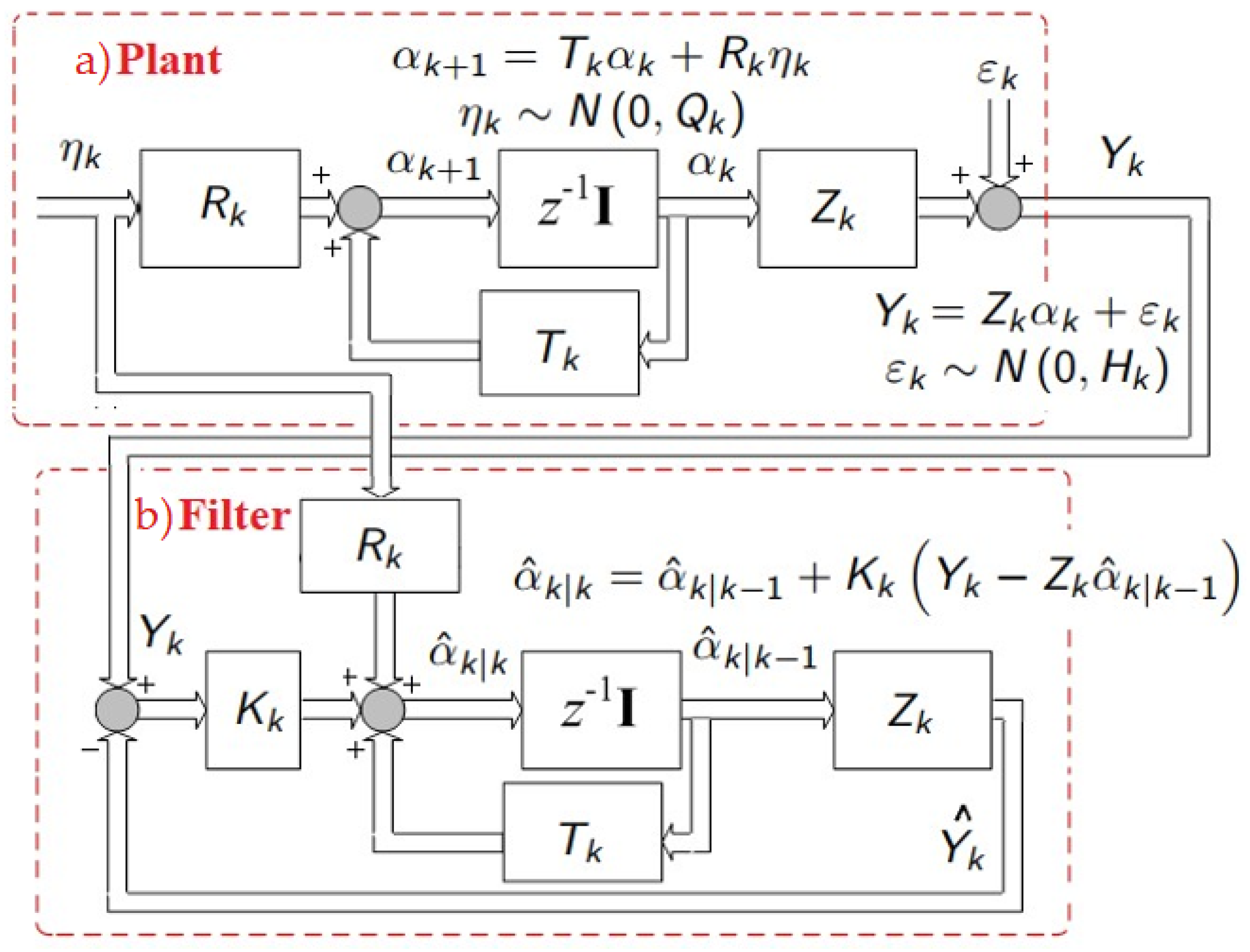
The Kalman filter is a powerful tool that combines different mathematical foundations such as dynamic systems, probability theory, and least squares to achieve control of systems with high measurement noise and provides the mathematical foundation of the following value. In Figure 1, the block algebra of the Kalman filter is shown. The original system is represented by the “Plant” with two noise sources, intrinsic noise ${\eta }_k$, and measurement noise ${\epsilon }_k$. The KF is based on the full-order observer represented at the bottom as the “Filter”, which consists of duplicating the mathematical model of the “Plant” whose inputs are the measurement vector $Y_k$ and the past estimated measurement vector ${\widehat{Y}}_k$, and then statistically weighted by the Kalman gain $K_k$, which defines the amount of noise contained in the output $Y_k$ at the instant $k$ [5,22]. The Kalman filter is originally discrete where the State Equation defines the model of the system (2) and the Measurement Equation (3), as follows:

$${\alpha }_k=T_k{\alpha }_{k-1}+R_k{\eta }_k, {\eta }_k\sim \mathrm{N}\left(0,Q_k\right),$$

(2)

$$Y_k=Z_k{\alpha }_{k-1}+{\epsilon }_k, {\epsilon }_k\sim \mathrm{N}\left(0,H_k\right),$$

(3)

where ${\alpha }_k$ is the current state vector, ${\alpha }_{k-1}$ is the previous state vector, $T_k$ is the system characteristic matrix, $R_k$ is the noise input matrix, and ${\eta }_k$ is the noise input vector with normal distribution with zero-mean and variance–covariance matrix $Q_k$, $Y_k$ is the measurement vector (time series data), $Z_k$ is the output state selection matrix, and ${\epsilon }_k$ is the measurement noises vector with normal distribution with zero-mean and variance–covariance matrix $H_k$.

The estimation of the State Equation at time $k$, due to the past observation in time $k-1$, called the Prediction Equation, is expressed by Equation (4), as follows:

$${\widehat{\alpha }}_{k|k-1}=T_k{\widehat{\alpha }}_{k-1|k-1}+R_k{\eta }_k,$$

(4)

where ${\widehat{\alpha }}_{k|k-1}$ is the estimated state vector at time $k$, due to the past observation in time $k-1$, and ${\widehat{\alpha }}_{k-1|k-1}$ is the previous estimated state vector at time $k-1$, due to time $k-1$.

Once the actual output $Y_k$ arrives, the Kalman filter updates the prediction of the State Equation, called the Update Equation, expressed by Equation (5), as follows:

$${\widehat{\alpha }}_{k|k}={\widehat{\alpha }}_{k|k-1}+K_k\left(Y_k-Z_k{\widehat{\alpha }}_{k|k-1}\right),$$

(5)

where ${\widehat{\alpha }}_{k|k}$ is the estimated state vector at time $k$, due to the observation at time $k$, ${\widehat{\alpha }}_{k|k-1}$ is the state estimated vector at time $k$, due to the previous observation at time $k-1$, $K_k$ is the Kalman gain matrix, $Y_k$ is the measurement vector, and $Z_k$ is the state selection output matrix.

The Kalman filter is a recursive algorithm whose purpose is to estimate the real state without noise. However, it also performs an estimation of the next state commonly used in forecasting approaches.

3.2. Forecasting Filtered Time Series

A properly filtered time series is reduced in complexity, facilitating the extraction of trends and harmonics of the DL forecasting methods. An important component of any neural network architecture, like LSTM or CNN, is that it allows the emulation of nonlinear systems by including small nonlinearities in the activation functions. Thus, these filter signals may be able to learn the complex patterns of the real model [24]. One of their disadvantages is the exploding gradient, which occurs when an RNN’s associated error is too small, making the training short and susceptible to being stopped at a local minimum when the hyperbolic tangent activation function is employed. On the contrary, when an activation function is activated near the extremes, a large associated error is assigned to this neuron, which may be ignored by the algorithm, causing a vanishing gradient [25]. Due to this situation, and looking to perform an adequate forecast, the LSTM and CNN architectures are among the most stable for approximating nonlinear systems employing a neural network training system [25,26].

Typically, metrics such as MSE, Pin-Ball loss [27], or loss entropy are employed to assess training effectiveness when using neural networks for time series forecasting [4].

3.3. Singular Spectrum Analysis

Singular spectrum analysis (SSA) is a widely used vision technique for extracting principal components from an image. The application of SSA in time series analysis begins with the well-known Hankelization process, which involves mapping a time series structured into an X matrix known as the Hankel matrix, in which X is a symmetric matrix whose diagonals from left to right are numerically parallel [9]. SSA’s methodology for this work consists of the following two main parts: training and forecasting.

3.3.1. Training

The Hankelization of a time series of length $N$ in an X matrix of $L$ columns and $K=N-L+1$ rows is performed with Equation (6), as follows:

$$\mathit{X}=\left[\begin{array}{ccccc}{X}_1& X_2& X_3& \cdots & X_L\\ X_2& X_3& X_4& \cdots & X_{L+1}\\ X_3& X_4& X_5& \cdots & X_{L+2}\\ ⋮& ⋮& ⋮& \ddots & ⋮\\ X_k& X_{k+1}& X_{k+2}& \cdots & X_N\end{array}\right]\in R^{K,L},$$

(6)

where $\mathit{X}$ is the Hankel matrix, also called the trajectory matrix, $x_i$ is the ith value of the time series, $N$ is the total data of the time series, $L$ is the width of the window of the time series, and $K$ is the number of windows for the time series. Matrix $\mathit{X}$ may not be square, therefore, it would not have eigenvalues. However, any rectangular matrix with linearly independent rows $\mathit{X}\in R^{K,L}$ admits a singular value decomposition (SVD), presented in Equation (7) as follows:

$$\mathit{X}=\mathit{U}{\mathit{\Sigma }\mathit{V}}^{\mathit{T}},$$

(7)

where $\mathit{U}\in R^{K,K}$ is a square matrix of dimension $K$, which contains the left singular vectors of matrix $\mathit{X}$, $\mathit{\Sigma }\in R^{K,L}$ is a diagonal matrix in which the singular values of matrix $\mathit{X}$ are located, and ${\mathit{V}}^{\mathit{T}}\in R^{L,L}$ is a transpose square matrix of dimension $L$, which contains the right singular vectors.

The vector of singular values ${\mathit{\sigma }}_{\mathit{L}}\in R^L$ is located on the main diagonal of matrix $\mathit{\Sigma }$, and is found by computing the eigenvalues of square matrix ${\mathit{X}}^{\mathit{T}}\mathit{X}$ using $\mathit{\sigma }$ = ${\mathit{\lambda }}^{0.5}$, where ${\mathit{X}}^{\mathit{T}}\mathit{X}\in R^{L,L}$ is the quadratic form of matrix $\mathit{X}$ and ${\mathit{V}}^{\mathit{T}}$ is the matrix of unit eigenvectors associated with the eigenvalues of quadratic matrix ${\mathit{X}}^{\mathit{T}}\mathit{X}$. Matrix $\mathit{U}$ is an orthonormal matrix that satisfies Equation (7). With the decomposition of matrix $\mathit{X}$, an approximation of the trajectory matrix $\widehat{\mathit{X}}$ can be reconstructed with the first $r$ singular values instead of all of the singular values in ${\mathit{\sigma }}_{\mathit{L}}$. The idea is to reconstruct the trajectory matrix $\mathit{X}$ only with the singular values that define the time series, thus excluding the singular values associated with noise and retaining those associated with trend and seasonality.

3.3.2. Forecasting

After obtaining the reconstructed time series through SSA, forecasting can be undertaken using either the recurrent or vector approaches, both of which are well-established methods within the SSA framework [9,10]. While vector forecasting generates a set of future values simultaneously by extending trajectory matrix $\mathit{X}$, recurrent forecasting employs a step-by-step prediction process to iteratively predict the future values, incorporating each new forecast back into the model for subsequent predictions. The recurrent forecasting starts with a linear regression approach, as described in Equation (8), as follows:

$$\mathit{A}\mathit{p}=\mathit{b};with\mathit{A}=\left[\begin{array}{ccccc}{x}_1& x_2& x_3& \cdots & x_{L-1}\\ x_2& x_3& x_4& \cdots & x_L\\ x_3& x_4& x_5& \cdots & x_{L+1}\\ ⋮& ⋮& ⋮& \ddots & ⋮\\ x_K& x_{K+1}& x_{K+2}& \cdots & x_{N-1}\end{array}\right]{\in R}^{K,L-1},\mathit{p}=\left[\begin{array}{c}{p}_1\\ p_2\\ p_3\\ ⋮\\ p_{L-1}\end{array}\right]\in R^{L-1},\mathit{b}=\left[\begin{array}{c}{x}_L\\ x_{L+1}\\ x_{L+2}\\ ⋮\\ x_N\end{array}\right]\in R^K,$$

(8)

where $\mathit{A}$ is trajectory matrix $\mathit{X}$ truncated from its last column, $\mathit{p}$ is a slope column vector of dimension $L$, and $\mathit{b}$ is the column vector truncated from the $\mathit{X}$ matrix to form the $\mathit{A}$ matrix. With $\mathit{A}$ and $\mathit{b}$ known, $\mathit{p}$ is founded by using Equation (8) and substituting matrix $\mathit{A}$ with its SVD: $\mathit{U}\mathit{\Sigma }{\mathit{V}}^{\mathit{T}}\mathit{p}=\mathit{b}$. To clear $\mathit{p}$, it is necessary to pre-multiply both sides of Equation (8) by the left pseudo-inverse of the SVD of $\mathit{A}$, called the left Moore–Penrose pseudo-inverse ${\mathit{A}}^{†}=\mathit{V}{\mathit{\Sigma }}^{-1}{\mathit{U}}^T$:$\mathit{V}{\mathit{\Sigma }}^{-1}{\mathit{U}}^T\mathit{U}\mathit{\Sigma }{\mathit{V}}^{\mathit{T}}\mathit{p}=\mathit{V}{\mathit{\Sigma }}^{-1}{\mathit{U}}^{T}b$. Recall that, since $\mathit{U}$ and $\mathit{V}$ are orthonormal, their inverses are equal to their transposes, therefore, ${\mathit{U}}^T\mathit{U}\approx \mathit{I}$, ${\mathit{\Sigma }}^{-1}\mathit{\Sigma }=\mathit{I}$, and ${\mathit{V}\mathit{V}}^{\mathit{T}}=\mathit{I}$, and the best approximation of $\mathit{p}$ is $\widehat{\mathit{p}}=\mathit{V}{\mathit{\Sigma }}^{-1}{\mathit{U}}^{\mathit{T}}\mathit{b}$. There are two possible cases due to the window width $L$, as follows: (a) underdetermined, when $K<L$, there are infinitely many solutions in $\mathit{p}$ to describe $\mathit{b}$; and (b) when $K>L$, there are not enough observations in $\mathit{b}$ to determine an exact solution in $\mathit{p}$.

Upon obtaining the slope approximation $\widehat{\mathit{p}}$, a newly updated matrix ${\mathit{A}}_{\mathit{i}}^{\mathit{f}\mathit{c}\mathit{a}\mathit{s}\mathit{t}}$ can be obtained from the current $\mathit{A}$ matrix. Then, this ${\mathit{A}}_{\mathit{i}}^{\mathit{f}\mathit{c}\mathit{a}\mathit{s}\mathit{t}}$ matrix is used to estimate a new output vector $\widehat{\mathit{b}}$. Nonetheless, owing to the Hankelization of the time series data, it becomes evident that solely the terminal element of $\widehat{\mathit{b}}$ provides an estimation pertinent to the forecasting horizon. This implies that the forecasted values are exclusively available for a one-step-ahead prediction. Algorithm 1 is designed to forecast the entire horizon forecast $\left(HF\right)$ by incrementally updating the forecast ${\mathit{f}}_{\mathit{c}\mathit{a}\mathit{s}\mathit{t}}$. The algorithm, in line 1, starts by executing a column shift operation on matrix $\mathit{A}$. This action omits the leftmost column, laying the foundation for the primary columns of the initial matrix ${\mathit{A}}_0^{\mathit{f}\mathit{c}\mathit{a}\mathit{s}\mathit{t}}$. Subsequently, in line 2, the extreme right column of matrix ${\mathit{A}}_0^{\mathit{f}\mathit{c}\mathit{a}\mathit{s}\mathit{t}}$ is replaced by the output vector $\mathit{b}$, thereby integrating the initial matrix ${\mathit{A}}_0^{\mathit{f}\mathit{c}\mathit{a}\mathit{s}\mathit{t}}$. In line 3, the initial estimated output vector ${\widehat{\mathit{b}}}_0$ is computed using the initial matrix ${\mathit{A}}_0^{\mathit{f}\mathit{c}\mathit{a}\mathit{s}\mathit{t}}$ and the slope approximation $\widehat{\mathit{p}}$. In line 4, a cycle while is applied for the entire length of the $HF$. In lines 5 and 6, matrix ${\mathit{A}}_{\mathit{i}}^{\mathit{f}\mathit{c}\mathit{a}\mathit{s}\mathit{t}}$ is updated with the precedent matrix ${\mathit{A}}_{\mathit{i}-1}^{\mathit{f}\mathit{c}\mathit{a}\mathit{s}\mathit{t}}$ and the previous estimated output vector ${\widehat{\mathit{b}}}_{\mathit{i}-1}$. In line 7, the current matrix ${\mathit{A}}_{\mathit{i}}^{\mathit{f}\mathit{c}\mathit{a}\mathit{s}\mathit{t}}$ is used to estimate vector ${\widehat{\mathit{b}}}_{\mathit{i}}$—notice that vector ${\widehat{\mathit{b}}}_{\mathit{i}}$ is an input. Finally, in line 8 the last forecast is updated, taking the last value into vector ${\widehat{\mathit{b}}}_{\mathit{i}}$.

Algorithm 1: Updating Fcast

Input: $HF$, $\mathit{A}$, b, $\widehat{\mathit{p}}$;$i=1$; Output: ${\mathit{f}}_{\mathit{c}\mathit{a}\mathit{s}\mathit{t}}$

(1)     ${\mathit{A}}_0^{\mathit{f}\mathit{c}\mathit{a}\mathit{s}\mathit{t}}[:,:-1]=\mathit{A}[:,2:]$

(2)     ${\mathit{A}}_0^{\mathit{f}\mathit{c}\mathit{a}\mathit{s}\mathit{t}}[:,-1]=\mathit{b}$

(3)     ${\widehat{\mathit{b}}}_0={\mathit{A}}_0^{\mathit{f}\mathit{c}\mathit{a}\mathit{s}\mathit{t}}\widehat{\mathit{p}}$

(4)     while $(i<HF)$ do

(5)        ${\mathit{A}}_{\mathit{i}}^{\mathit{f}\mathit{c}\mathit{a}\mathit{s}\mathit{t}}[:,-1]={\widehat{\mathit{b}}}_{\mathit{i}-1}$

(6)        ${\mathit{A}}_{\mathit{i}}^{\mathit{f}\mathit{c}\mathit{a}\mathit{s}\mathit{t}}[:,:-1]={\mathit{A}}_{\mathit{i}-1}^{\mathit{f}\mathit{c}\mathit{a}\mathit{s}\mathit{t}}[:,2:]$

(7)        ${\widehat{\mathit{b}}}_{\mathit{i}}={\mathit{A}}_{\mathit{i}}^{\mathit{f}\mathit{c}\mathit{a}\mathit{s}\mathit{t}}\widehat{\mathit{p}}$

(8)        ${\mathit{f}}_{\mathit{c}\mathit{a}\mathit{s}\mathit{t}}\left[i\right]={\widehat{\mathit{b}}}_{\mathit{i}}[-1]$

(9)        $i=i+1$

(10)   End

3.4. Forecasting Performance Measures

The proposed forecasting method is evaluated by the mean average percentage error (MAPE) [11,28], RMSE, and directional accuracy metric (DA) [29]. These metrics are shown in Equations (9)–(11), as follows:

$$MAPE=\frac{100}{h}\sum _{t=1}^h\frac{\left|{y_t-\widehat{y}}_t\right|}{\left|y_t\right|},$$

(9)

where $y_t$ is the actual observation, ${\widehat{y}}_t$ is the actual prediction, and $h$ is the length of the forecast horizon.

The MAPE is useful to intuitively show the performance; nevertheless, it fails when the observed value and the forecast are near-zero. To avoid this situation, the RMSE [28] is used to provide a standardized measure of the performance, as follows:

$$RMSE={\left(\frac{1}{h}{\sum }_{t=1}^h{\left(y_t-{\widehat{y}}_t\right)}^2\right)}^{\frac{1}{2}},$$

(10)

The RMSE performance indicator, while it is a valuable tool, lacks the intuitive clarity of MAPE. Nevertheless, RMSE effectively addresses issues related to both over-forecasting and under-forecasting, particularly when dealing with values approaching zero. However, it is important to note that RMSE and MAPE primarily emphasize absolute numerical accuracy and may not comprehensively capture the dynamism inherent in the forecasting processes.

The directional accuracy (DA) metric focuses on the correct direction of predictions rather than their absolute numerical accuracy. This is particularly valuable in situations where correctly predicting the change in direction is critical. In other words, the DA provides a clearer assessment of a model’s ability to make accurate directional forecasts, which can be especially important in decision making and applications where knowing the correct direction trend is as important as precise numerical values.

$$DA=\frac{100}{h}{\sum }_{t=1}^h{a}_t with a_t=\left\{\begin{array}{c} \begin{array}{cc}1& \left(y_t-y_{t-1}\right)\left({\widehat{y}}_t-{\widehat{y}}_{t-1}\right)\ge 0\end{array}\\ \begin{array}{cc}0 & otherwise\end{array}\end{array}\right.,$$

(11)

where $a_i$ is a piecewise function with a value one or zero, $y_{t-1}$ is the past observation, and ${\widehat{y}}_{t-1}$ is the past prediction.

4. FMFRA Methodology

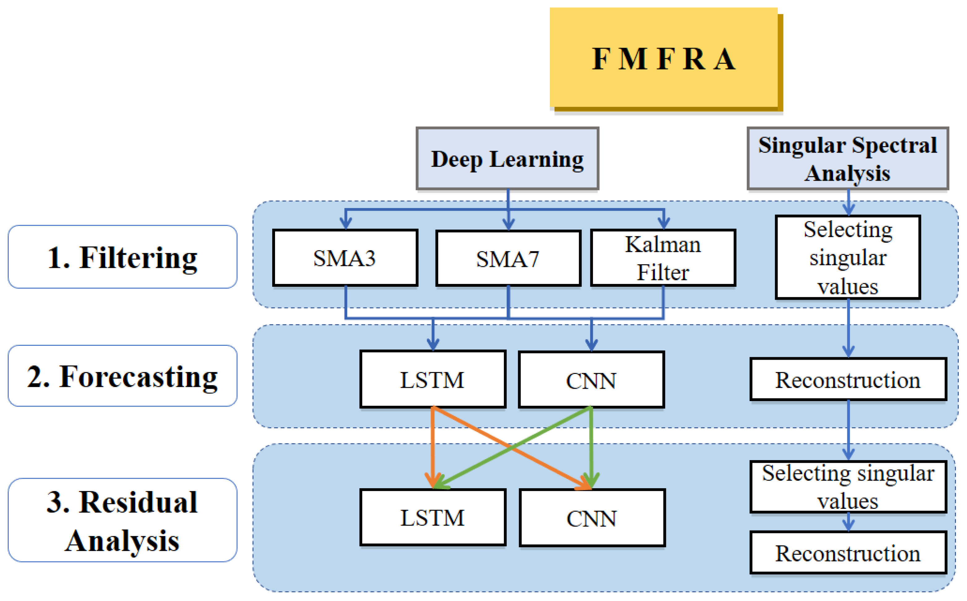
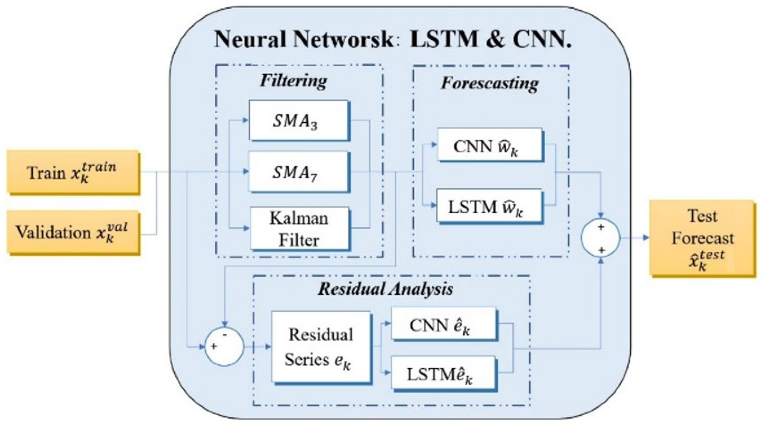
There is no general forecasting method that provides the best results, due to the complexity of the time series and its intrinsic noise. In Figure 2, we present the methodology proposed here, which resolves these issues by selecting between the following two models: DL and SSA. Both of these models have the following three phases: filtering, forecasting, and residual analysis. In the FMFRA-DL model, the first phase is smoothing the time series in parallel by the three filters with better performance in the previous experimentations. With a filtered series, the learning task for the second phase is reduced to finding trends and principal seasonalities by repeating LSTM and CNN $m$ times until finding the best forecast validation. Finally, in the residual analysis phase, the filtered series is subtracted from the original series to obtain a residual series without trends and principal seasonalities. Only the remaining seasonalities will be found by a different configuration of LSTM and CNN. In the FMFRA-SSA model, an automatic search is applied first to select the principal singular values. In the second phase of SSA, the reconstruction of the trajectory matrix $\widehat{\mathit{X}}$ with the selected singular values is obtained. Finally, for the residual analysis phase, the reconstructed time series is subtracted from the original to obtain the residual time series, and another automatic search of singular values is performed to improve the first forecasting. Section 4.1 and Section 4.2 describe the three phases of each method.

Algorithm 2 presents the FMFRA in full form. The inputs are the time series (all of the values in the time series) and $HF$, while the outputs are the forecasts and the performance measures ($Fcast$ and Performance_Measures). This algorithm executes the following two principal methods: FMFRA-DL and FMFRA-SSA. The former corresponds to DL application with LSTM and CNN. Previously, three filters were applied. On the other hand, FMFRA-SSA is the application of this methodology using SSA (the three phases of Figure 2). FMFRA-DL starts, in line 1, with a simple normalization process. Line 3 involves dividing the time series, and line 6 applies $k$ filters (SMA3, SMA7, and KF) to the training set, obtaining the filtered signal and the residual signal in lines 7 and 8, respectively. Subsequently, line 9 executes the function searchingL&C, as presented in Algorithm 3. This function finds the best training model (according to the performance in the validation forecast phase) for the filtered series and the residual series. This algorithm searches for the best model by applying LSTM and CNN $m$ times (as presented in Section 4.1.2). Lines 11 and 12 add the four possible filtered and residual forecast result combinations. From lines 13 to 16, the optimal forecast combination for the filtered and residual series is determined. FMFRA-SSA starts in line 18. Then, in line 19, function fmfra-ssa is executed to determine the mean square error (MSE), the parameters, and the forecast SSAfast by the application of the classical SSA method. This function is presented in Algorithm 4. Line 20 starts the selection of the best forecast between FMFRA-DL and FMFRA-SSA. In line 21, the function append is applied. This function appends the two best forecasts in the list of Fcastcases. Line 22 applies the function minpos to find the position of the lowest MSE in the list of Fcastcases. In line 23, the best model is determined by knowing the position of the best model, which is stored in the variable SelectedFcast. Then, in line 24, the function fcast is executed. This function concatenates the training and validation sets to forecast the test with the SelectedFcast. To correctly show the forecast in daily cases, data denormalization is applied, in line 26, by the function datadenormalization. This forecast is stored in $Fcast$. Finally, in line 28, the MAPE, DA, and RMSE are computed by the function performance_measures.

Algorithm 2: FMFRA

Input: $HF$, Timeseries.

Output: $Fcast$, Performance Measures

(1) data_normalization()//The time series are normalized: 0 to 1000.

(2) //Training data, Validation data, and Test data are obtained from the time series.

(3) split_series()

(4) //FMFRA-DL generates twelve forecasting cases

(5) //Filters are applied to the time series

(6) for each filter $k$ do:

(7)  Filtersignal = filter(Timeseries)

(8)  Residualsignal = Timeseries − Filtersignal

(9)  BestL, BestC = searchingL&C(Filtersignal,Residualsignal)

(10) End

(11) FcastValL = sum(BestL)//best filter signal + residual signal of LSTM

(12) FcastValC = sum(BestC)//best filter signal + residual signal of CNN

(13) AllFcast = appen(FcastValL, FcastValC)

(14) AllMSE = error(FcastValL, FcastValC)

(15) BestMSE = minpos(AllMSE)//find the position with the minor MSE

(16) Bestfcast = AllFcast[bestMSE]//use the bestMSE to obtain the best forecast

(17) //end of FMFRA-DL

(18) //FMFRA-SSA generates $L$ and $r$ parameters for forecasting

(19) MSE,SSAfcast = fmfra-saa(Timeseries)

(20) //Choice best Forecasting between FMFRA-DL and FMFRA-SSA.

(21) Fcastcases = append(Bestfcast, SSAfcast)

(22) MSEcases = minpos(Fcastcases)//find the method with lowest MSE

(23) SelectedFcast = Fcastcases[MSEcases]

(24) FcastTest = fcast(SelectedFcast)

(25) //The Test forecast is denormalized to get the Forecasting Test

(26) $Fcast$ = datadenormalization(FcastTest)

(27) //MAPE, DA, and RMSE are calculated for the final forecast

(28) Performance_Measures = performance_measures($Fcast$)

Algorithm 3: searchingL&C function

(1) searchingL&C()

(2) //repeats $m$ executions for filter signal or residual signal

(3) for each iteration $m$ do:

(4)   FcastL[m] = lstm(Filtersignal or Residualsignal)//Forecasting LSTM

(5)   MSEL[$m$] = error(FcastL[$m$])//mse of LSTM

(6)   FcastC[$m$] = cnn(Filtersignal or Residualsignal)//Forecasting CNN

(7)   MSEC[$m$] = error(FcastC[$m$])//mse of CNN

(8)   BestL = min(MSEL[m])//best LSTM for filter signal or residualsignal

(9)   BestC = min(MSEC[m])//best CNN for filter signal or residualsignal

(10) End

(11) return BestL, BestC

(12) End//End function

Algorithm 4: fmfra-ssa function

(1) fmfra-ssa()

(2)  Topwindow = size(Timeseries)/2

(3)  SSAfcast = random[$HF$]//Randomly generate a solution with the size of $HF$

(4)  MSE = error(SSAfcast)

(5)  for $i$ = 2 to Topwindow do:

(6)    Window = $i$

(7)    $X$ = hankelization(Timeseries, Window)

(8)    $\sigma$ = SVD($X$)

(9)    $SL$ = size($\sigma$)

(10)     for $j$ = 1 to $SL$ do:

(11)    Fcast, MSESSA = fcast($i$, $j$)//function generates 2 parameters

(12)    if MSESSA $\le$ MSE then:

(13)        MSE = MSESSA

(14)        SSAfcast = Fcast

(15)    End

(16)     End

(17)  End

(18) return MSE, SSAfcast

(19) End//End function

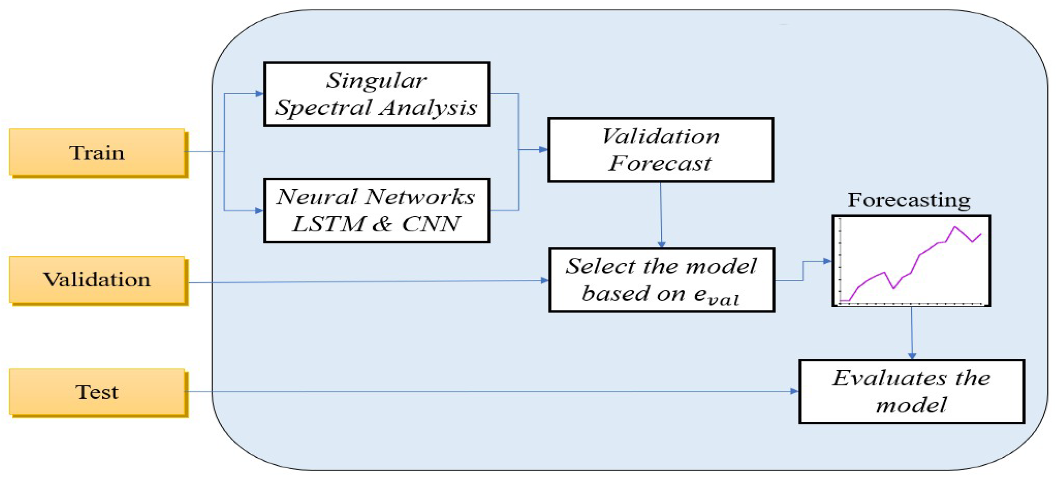
The time series of each country is normalized to correctly measure the forecast performance between countries with different populations, and the time series is split into training, validation, and testing. In Figure 3, the training of the two models is evaluated by the validation set by the MAPE, RMSE, and DA. The forecast validation with the better performance is chosen to make a forecast test, which is conducted using both the training and validation sets to measure the test performance.

The methods SSA and DL exhibit distinct specializations, sensitivities to noise, and versatile approaches for handling the complexities inherent in time series data analysis. While the DL method excels at extracting crucial patterns from historical data stored in its memory, the SSA method assigns similar weights to all of the data points within its trajectory matrix. Consequently, DL is more suitable when dealing with time series datasets with sufficient representative data [23,30]. Nevertheless, it fails for time series that are too short or too noisy. Conversely, SSA has a strength in discerning and truncating irrelevant information and allows for satisfactory validation forecasts [9].

4.1. Deep Learning by LSTM and CNN

Deep learning has been shown to be exceptionally well-suited for addressing and surpassing the other methods in several areas [30]. This approach is particularly successful in handling problems where solutions evolve dynamically over time, for instance, in applications like stock market prediction [26,31], weather forecasting [24], and tracking newly confirmed cases of COVID-19 [17,30].

As shown in Figure 4, the training set undergoes a filtering process, resulting in the creation of the following three new series: $SM{A}_3$, $SM{A}_7$, and $KF$. These filtered series are the foundation for generating two validation forecasts, including one for LSTM and another for CNN. Concurrently, the residual series $e_k$ leads to generating two additional validation forecasts, including one for LSTM and another for CNN. Finally, the results from both validation forecasts are combined for further analysis.

Consequently, this process yields a total of the twelve models, as shown in

Table 1. Combinations of the available models for the FMFRA-DL method.

Filtering	Forecasting	Residual Analysis
${SMA}_3$	LSTM	LSTM
		CNN
	CNN	LSTM
		CNN
${SMA}_7$	LSTM	LSTM
		CNN
	CNN	LSTM
		CNN
Kalman Filter	LSTM	LSTM
		CNN
	CNN	LSTM
		CNN

.

4.1.1. Filtering Phase in FMFRA-DL

The filter phase focuses on isolating the trend and primary seasonalities within the data series. The filter achieves the attenuation of the complexity of the time series and mitigates the noise elements, resulting in a purified data stream $w_k^{train}$ ready for subsequent analysis. Throughout our experimental process, a variety of filters were tested for efficacy. Remarkably, the $SMA3$, $SMA7$, and $KF$ filters emerged as the frontrunners, exhibiting a superior performance in defining the daily case trends of COVID-19 in the time series.

4.1.2. Forecasting Phase in FMFRA-DL

Once the time series has been filtered, a validation forecast is executed using LSTM and CNN methods to determine the best possible forecast, through the ensuing steps, as follows:

1.

A transformation of the filtered series data $w_k^{train}$ is applied to facilitate supervised learning, akin to the Hankelization discussed in Section 3.3. A window width of eight is employed, corresponding to the days of the week plus one additional day. Consequently, the DL method is furnished with data from the preceding seven days as parameters, and the output on the eighth day is predicted based on these values.

2.

By employing supervised learning, both of the models are trained according to the best architectures identified during our experimental process.

Table 2. Architectures for LSTM and CNN for filtering time series.

Architecture	Input Layer		Hidden Layer	Output Layer
LSTM	7 LSTM		42 LSTM	1 RNN
CNN	50 CNN	Pooling size: 2	50 RNN	1 RNN

displays the configurations for the three layers of both the LSTM and the CNN architectures.

Each architecture uses a batch size of 10. The input layer employs a ReLU activation function, the hidden layer utilizes a hyperbolic tangent function, and the output layer applies a ReLU function. The models are trained over 50 epochs. For the architecture of CNN, the input layer has a MaxPooling with size two in order to reduce dimensionality and noise.

3.

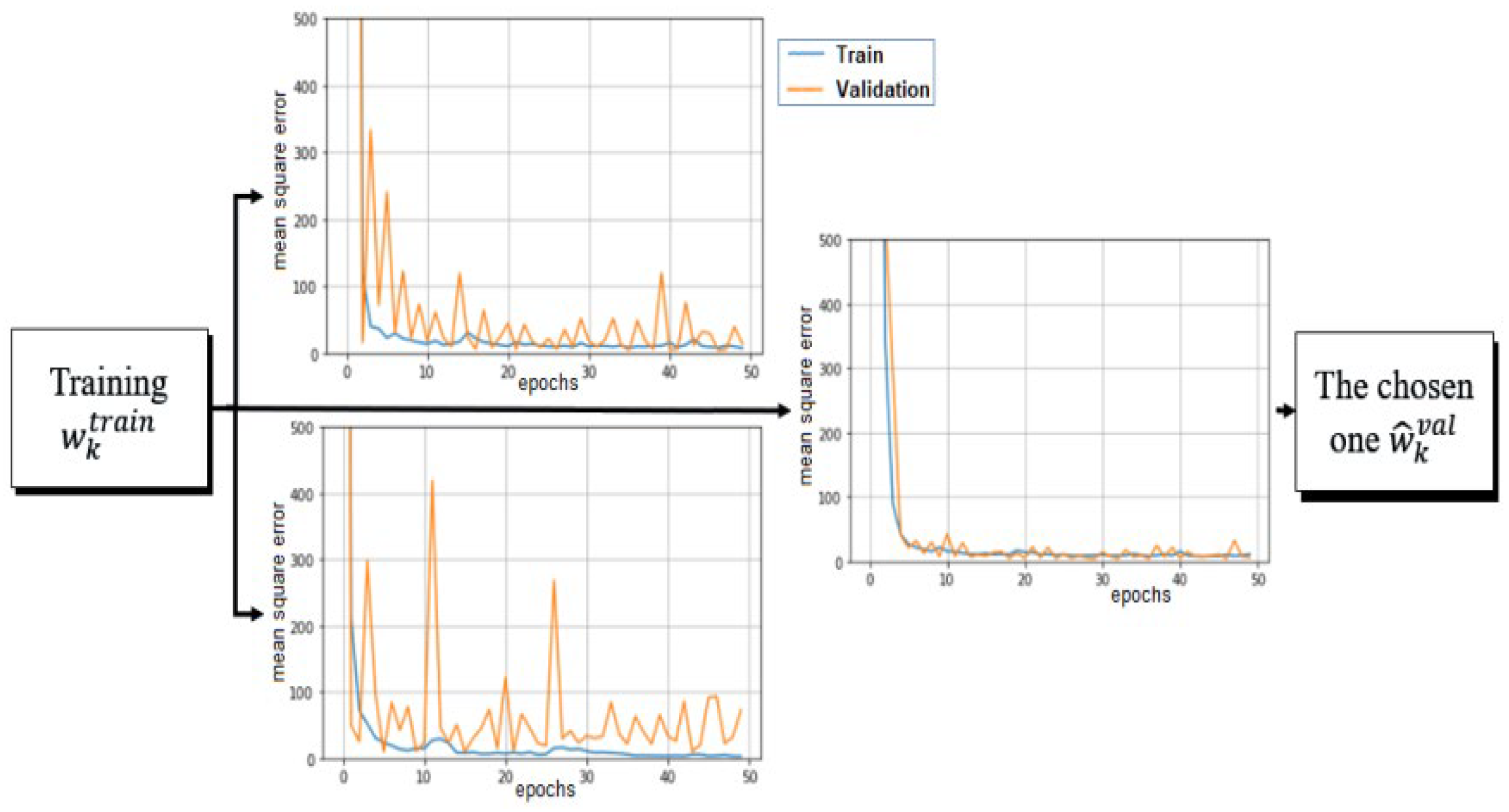
The variability of the predictions generated by these configurations is attributed to the vanishing and exploding gradients that occur due to the LSTM gates and also to the intermediate CNN and LSTM layers. This phenomenon stems from the random initialization of the initial weights. To enhance the robustness and reduce the uncertainty associated with the predictions generated by the LSTM and CNN models, a straightforward solution is implemented. The training process is executed $m$ times, and only the best training run for the LSTM is retained. Likewise, a search is conducted to identify the optimal training run within the CNN architecture.

Figure 5 shows an instance with $m=3$, showcasing 3 forecasting evaluations for LSTM using MSE along 50 epochs, where the best of them is shown on the right-hand side. The training performance is shown in blue, while the validation performance is in orange. Different training scenarios are generated by replicating the model training process with identical input time series and configurations (as detailed in Table 2). On the right-hand side of this figure, the training run with the best performance on the validation set is chosen to forecast the test set, while the other two training executions on the left-hand side are discarded. Section 5.2 delineates the outcomes of this iterative training approach, emphasizing the selection of the training process with the highest forecast validation performance as a strategy to diminish the variance in test prediction.

4.1.3. Residual Analysis Phase in FMFRA-DL

The residual series $e_k^{train}$ are obtained by subtracting the filtered series $w_k^{train}$ from the original time series $x_k^{train}$, resulting in a series without a trend and characterized by minor seasonal fluctuations and noise components. A comprehensive search to identify the best $MSE$ within the validation forecast phase is undertaken for this residual series $e_k^{train}$, adhering to the parameters specified in

Table 3. Architectures for LSTM and CNN for the residual time series forecasting.

Architecture	Input Layer		Hidden Layer	Output Layer
LSTM	7 LSTM		42 LSTM	1 RNN
CNN	21 CNN	Pooling size: 2	50 RNN	1 RNN

for each architecture. The input layer employs a ReLU activation function, the hidden layer utilizes a hyperbolic tangent function, and the output layer applies a ReLU function. The models are trained over 60 epochs.

4.2. Singular Spectrum Analysis

The singular spectral analysis method is an ideal tool for forecasting the onset of a pandemic, especially in scenarios where historical data are scarce, to facilitate accurate predictions through DL methods [9,10]. This method is crucial for clearly identifying the underlying trends and seasonality from the data, allowing for a greater certainty of the future. Besides, the efficacy of SSA remains high, as long as there are no abrupt shifts in the parameters defining the pandemic’s expansion. 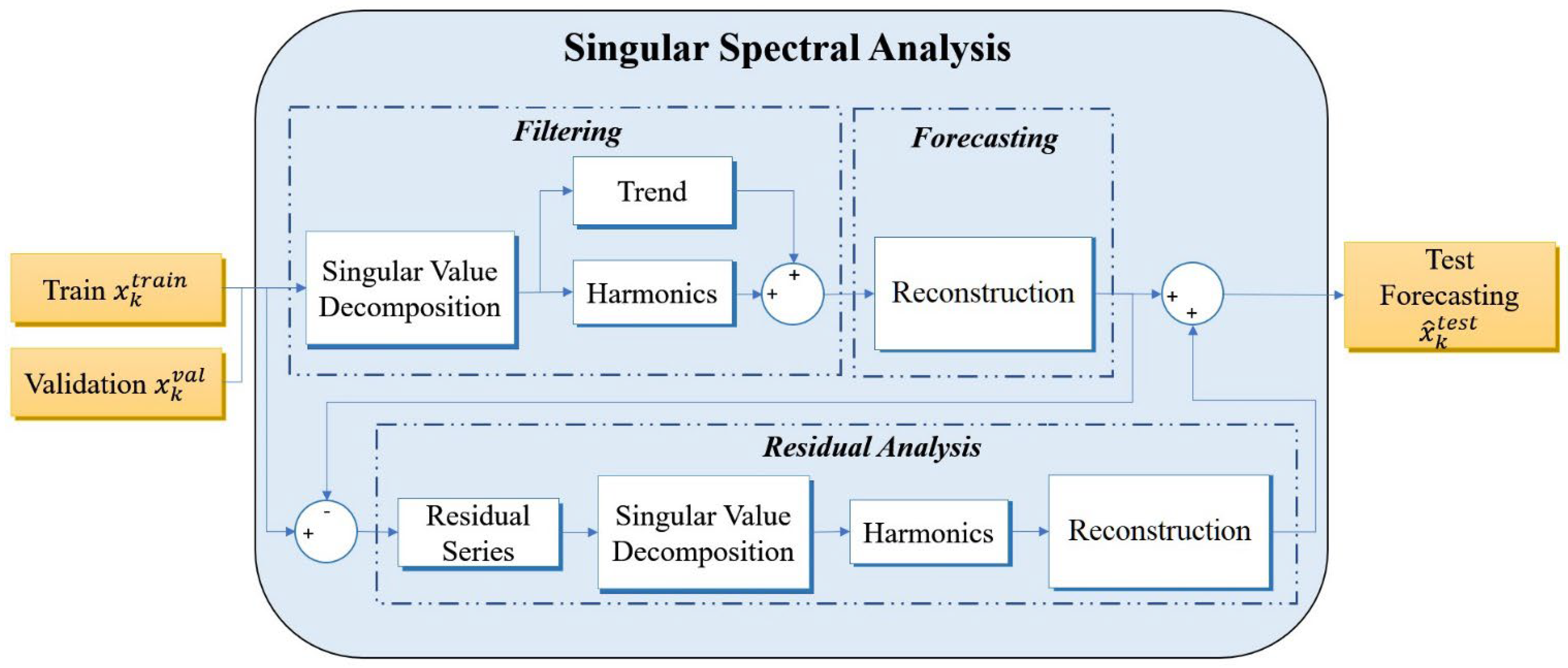Figure 6 presents the structural framework of Model 2, which focuses on SSA. In this approach, the time series $x_k^{train}$ undergoes the training process in order to decipher the inherent trends and dominant harmonics, which are subsequently updated, as shown in Algorithm 1. All of the possible window widths $L$ and singular values selected ${\sigma }_r$ are tested, aiming to generate a reliable estimation of the validation set ${\widehat{x}}_k^{val}$. This procedure is dedicated to identifying the estimation that exhibits the pinnacle of performance indicators RMSE and DA. This optimal estimation is then harnessed to reconstruct an estimated training set ${\widehat{x}}_k^{train}$, which is subtracted from $x_k^{train}$ to obtain the residual series $e_k^{train}$. During the residual analysis phase, a renewed quest is undertaken to isolate the additional harmonics that can enhance the accuracy of the validation forecast ${\widehat{x}}_k^{val}$. As a concluding step, the training set $x_k^{train}$ and the validation set $x_k^{val}$ are concatenated to form trajectory matrix $\mathit{X}$. Following this, a test forecast ${\widehat{x}}_k^{test}$ is calculated utilizing Algorithm 1, aligned with the optimal configuration discerned in the validation set, thereby promising a more accurate and reliable forecast.

4.2.1. Filtering and Forecasting Phase

For this phase, the time series is split into training, validation, and testing sets, and the first two are used to find the best approximation of the validation set ${\widehat{x}}_k^{val}$. This involves a meticulous exploration of the potential combinations of window width $L$, and singular values selected ${\sigma }_r$, to obtain the configuration that gives the most accurate forecasting results in the validation set $x_k^{val}$.

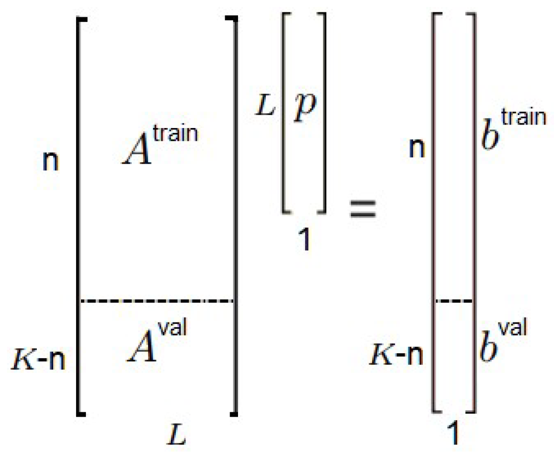
Figure 7 visually elucidates the training and validation sets represented in linear regression equations. Initially, the training set $x_k^{train}\in {\mathbb{R}}^{n+L}$ and the validation set $x_k^{val}\in {\mathbb{R}}^{K-n+L}$ are concatenated and undergo a Hankelization process to form a trajectory matrix $\mathit{A}\in {\mathbb{R}}^{K,L}$, which is further depicted in Equation (8). In the pursuit of identifying an estimated slope $\widehat{p}$, an $SVD$ is applied to each matrix ${\mathit{A}}^{train}\in {\mathbb{R}}^{n,L}$, generated by a window width $L$. It is imperative to note that, during our experimental phase, $L$ varied from seven to forty, beyond which there was no significant enhancement in the forecast performance. Utilizing the estimated slope $\widehat{p}$, an estimated validation forecast ${\widehat{b}}^{val}\in {\mathbb{R}}^{K-n}$ can be computed. This computation involves substituting ${\mathit{A}}^{train}\in {\mathbb{R}}^{n,L}$ with ${\mathit{A}}^{val}\in {\mathbb{R}}^{K-n,L}$, hence, yielding the following equation: ${\widehat{b}}^{val}=A^{val}\widehat{p}$.

To evaluate the performance of each validation forecast ${\widehat{b}}^{val}$, the RMSE is used. The accuracy across various configurations of window $L$ with the possible singular values ${\sigma }_r$, where $r$ is the number of singular values, is chosen. The next step is to truncate singular values one by one to obtain the forecast validation from $r$ = 1 to $r$ = $L$, and, for each validation forecast, an RMSE is obtained. Ultimately, the most suitable pairing of $L$ and $r$ is identified to obtain the best ${\widehat{b}}^{val}$. Next, $A^{train}$ and $A^{val}$ are concatenated to make the test forecast using Algorithm 1.

4.2.2. Residual Analysis Phase

This adaptation of the SSA method introduces a residual analysis, distinguishing it from the conventional SSA technique. This process involves the reconstruction of the time series, guided by the most compatible combination of $L$ and ${\sigma }_r$, identified during the initial phases of analysis. The newly reconstructed time series ${\widehat{x}}_k$ is then subtracted from the original time series $x_k$ (a concatenation of the $x^{train}$ and $x^{val}$ time series), to obtain the residual time series, $e_k$, through Equation (12), as follows:

$$e_k=x_k-{\widehat{x}}_k,$$

(12)

where $e_k$ is the residual time series, $x_k$ is the original time series, and ${\widehat{x}}_k$ is the reconstructed time series, with the $L$ and ${\sigma }_r$ founded in the last phase.

With the residual time series available, a subsequent round of the automated $SSA$ method is employed, albeit with a notable difference, as follows: the singular values of this residual series are devoid of trend components, containing only harmonics and noise elements. To formulate the final test forecast, the preliminary test forecast, which encompasses trend and harmonic components, is complemented by the harmonics discerned through the residual analysis. This comprehensive approach ensures a more precise forecast than the conventional SSA method.

5. Experimentation and Results

In this section, we present the outcomes of the proposed FMFRA method. The focus centers on evaluating the performance of the following two primary forecasting models: $SSA$ and DL. The evaluation metrics include MAPE, RMSE, and DA, which provide insights into the strengths and limitations of each filter technique and model architecture applied within the FMFRA framework. We have assessed this method using time series of daily COVID-19 cases, taken from four countries of American continent, which are the countries with a higher population. The data cover multiple stages of the pandemic, as follows: the onset, the peak of infections, and one year after. This comprehensive timeframe allows for a thorough assessment of the proposed forecasting method in different epidemiological contexts from March 2020 to May 2021. Regarding the data preparation prior to model training, we do not apply any specific transformation to the data. FMFRA operates on an unaltered dataset, and the final forecasts are also made using the daily case numbers as they are. Thus, this approach ensures that the predictions provided by FMFRA are directly interpretable in the context of the original data, maintaining the integrity and real-world relevance of the forecast results.

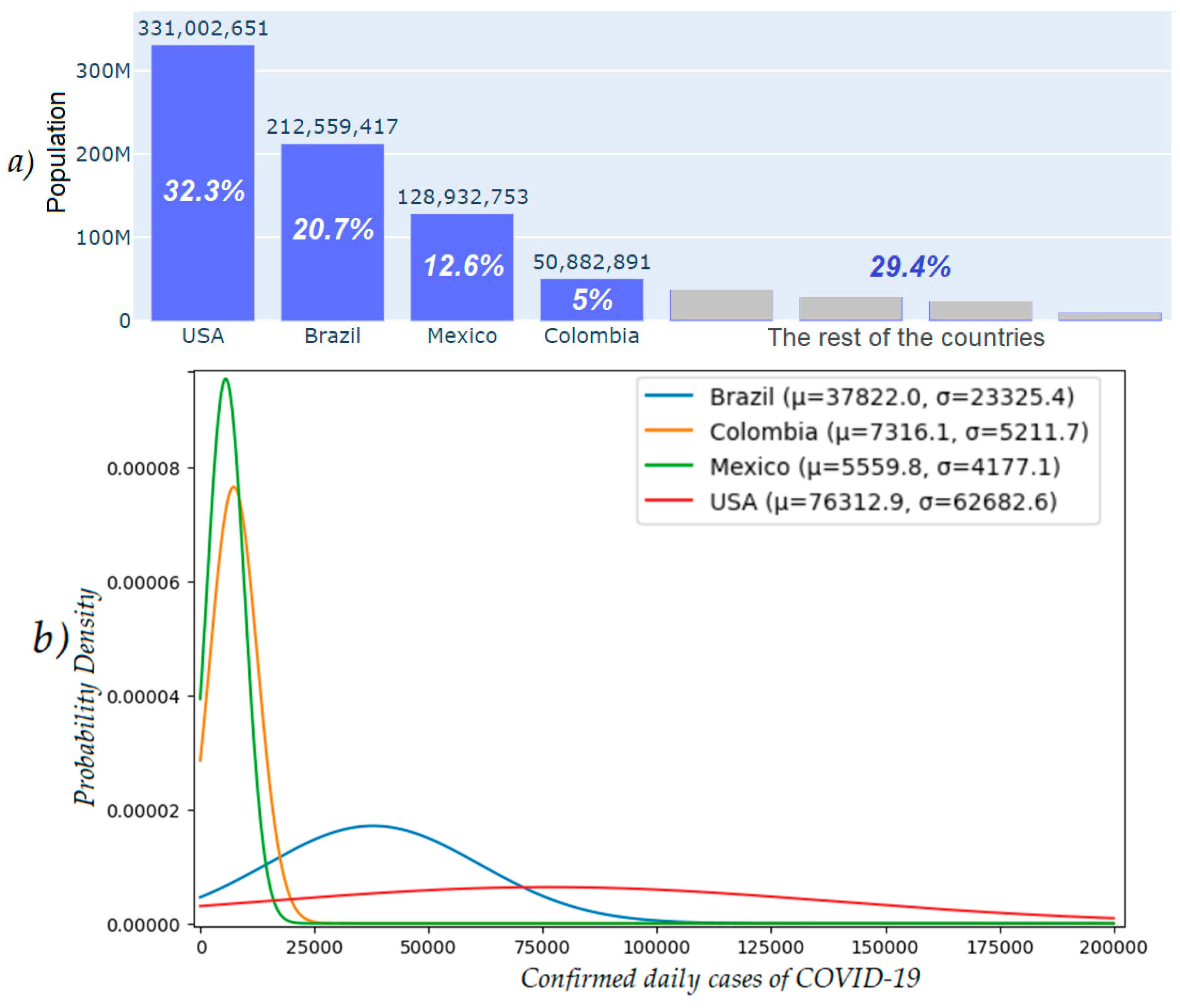
Figure 8 offers a comprehensive comparison of the population distribution and COVID-19 incidence in these key American countries. Figure 8a displays a bar graph depicting the 2020 population of the most populous countries in the American continent, being the United States, Brazil, Mexico, and Colombia, which are highlighted in blue. This visual representation underscores the prominence of these countries in terms of their population weight on the American continent. Complementing this view, Figure 8b presents gaussian distribution curves depicting the daily new COVID-19 cases for these countries, providing a clear perspective on the variance of COVID-19 cases in terms of frequency and distribution in each country. These two visualizations offer a deeper understanding of how the population density may correlate with the spread of the virus.

The data were normalized to ensure a fair comparison among the countries and to mitigate the impact of differences in population and case magnitudes. This normalization adjusted the time series to a scale from 0 to 1000, enabling an equitable assessment of each country. These data properties lay the foundation for the evaluation of the FMFRA approach.

A notable cornerstone of our research lies in our endeavor to mitigate the impact of noise during the model training phase. To achieve this objective, we tested the effectiveness of SMA and KF filters in Section 5.1. Subsequently, the present work explores the process of selecting the optimal validation forecast through the repetition of $m$ model runs, as discussed in Section 5.2. In addition, we contrast the results obtained from FMFRA with the following state-of-the-art forecasting methods: SSA automatic, XGBoost, RFR, and LR. In Section 5.3, we analyze the results in the following three distinct timeframes: at the onset, at the peak of infections, and one year into the pandemic.

5.1. Time Series Filtering

Mexico and other neighboring countries share geographic proximity and possible COVID-19 effects. Mexico shares its border with the USA, while Colombia neighbors Brazil. This geographical closeness often results in greater similarity in time series data, whereas differences may become more pronounced when comparing data from distant countries. This inherent property suggests that countries with similar profiles may achieve more accurate forecasts when employing similar filters and methodologies. The effectiveness of signal filtering for DL in this work depends on the adequate split of the time series into two time series: filtered and residual time series. The next subsection presents the results of the experimentation with SMA and KF filters.

5.1.1. Simple Moving Average

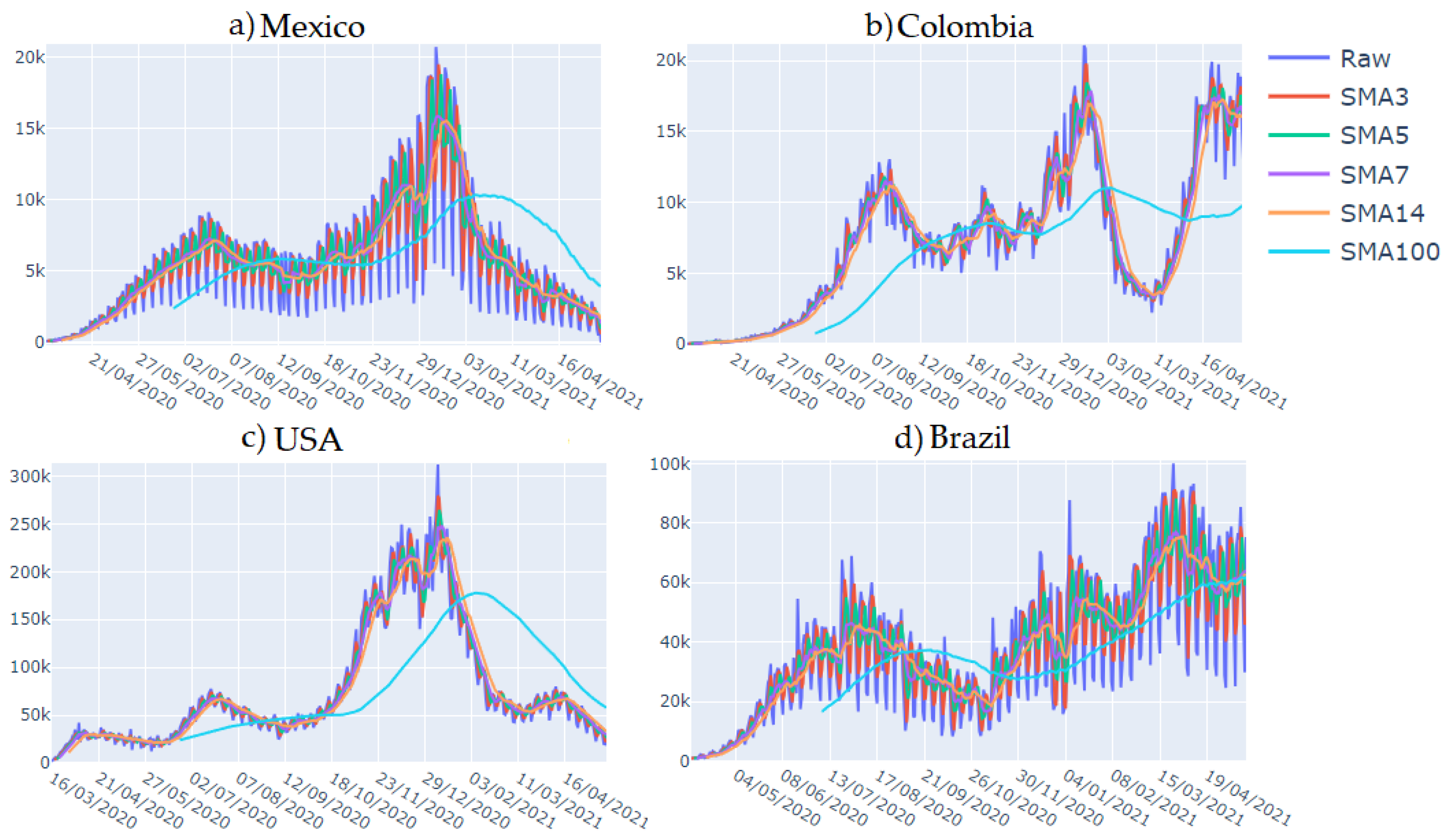
We applied ${SMA}_n$ filters to different time series of the countries mentioned previously to enhance the forecast, where $n=3,5,7$, and $100$. We found that the resulting filtered time series are more similar when $n$ is increased, allowing for the appreciation of general patterns. Figure 9 displays the following four countries analyzed in this work: Mexico, the United States, Colombia, and Brazil. In the graph, the raw time series is represented in deep blue, the $SM{A}_3$ in red, $SM{A}_5$ in green, $SM{A}_7$ in purple, $SM{A}_{14}$ in orange, and $SM{A}_{100}$ in sky blue. The time series spans from March 2020 to May 2021.

The best results in the validation forecast were obtained with $n=$ 3 and $n=$ 7. A possible explanation for this could be that, for daily cases, $SM{A}_7$ calculates the average over the entire week, capturing the weekly seasonality of the time series. On the other hand, $SM{A}_3$ could correspond to the size of the weekends, helping to smooth out the abrupt peaks and atypical data points usually occurring during holidays.

5.1.2. Kalman Filter

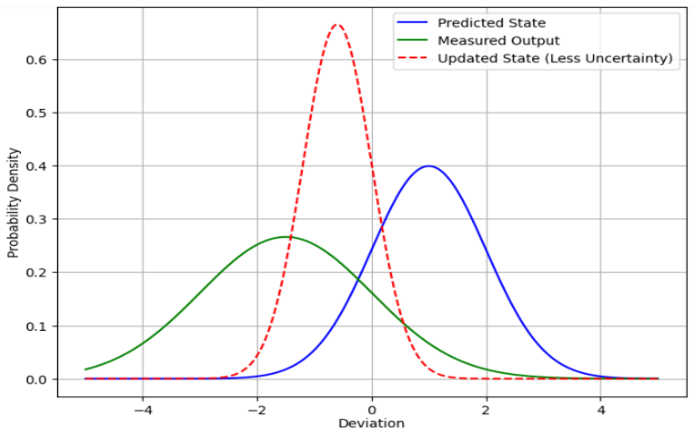
Based on the outcomes obtained from the $SMA$ filters, we found that the forecast performance improves when utilizing filters that effectively isolate the underlying trend and primary seasonal patterns. Furthermore, we employed the KF due to its remarkable capacity to reduce uncertainty. As shown in Figure 10, the process involves an initial predicted state in blue. Subsequently, this predicted state is refined through an update step, incorporating the measured output in green. This enhancement is achieved by applying a weighting factor known as Kalman gain ($K_k$). The $K_k$ was tailored to the noise in the variance–covariance matrix, and the system model, diminishing the uncertainty associated with the update state, is shown in the red dashed line [5,23,32].

In the realm of time series forecasting, it is common to provide the time series without its mathematical model. However, the Kalman filter emerges as a remarkably potent tool precisely in situations where an effective mathematical model is absent [7,22,23]. In the absence of such a model, we need to treat the mathematical model as akin to a random walk, described as follows: ${\alpha }_{k+1}={\alpha }_k+{\eta }_k$ and $y_k={\alpha }_k+{\epsilon }_k$, where ${\alpha }_{k+1}$ is the state vector at the next instant, ${\alpha }_k$ is the state vector at the current instant, ${\alpha }_k~N(0,Q_k)$ is a random number following a normal distribution with a mean of 0 and variance–covariance matrix $Q_k$, $y_k$ is the state vector measurement, and ${\epsilon }_k~N(0,H_k)$ is the measurement of noise following a normal distribution with a mean of 0 and variance–covariance matrix $H_k$.

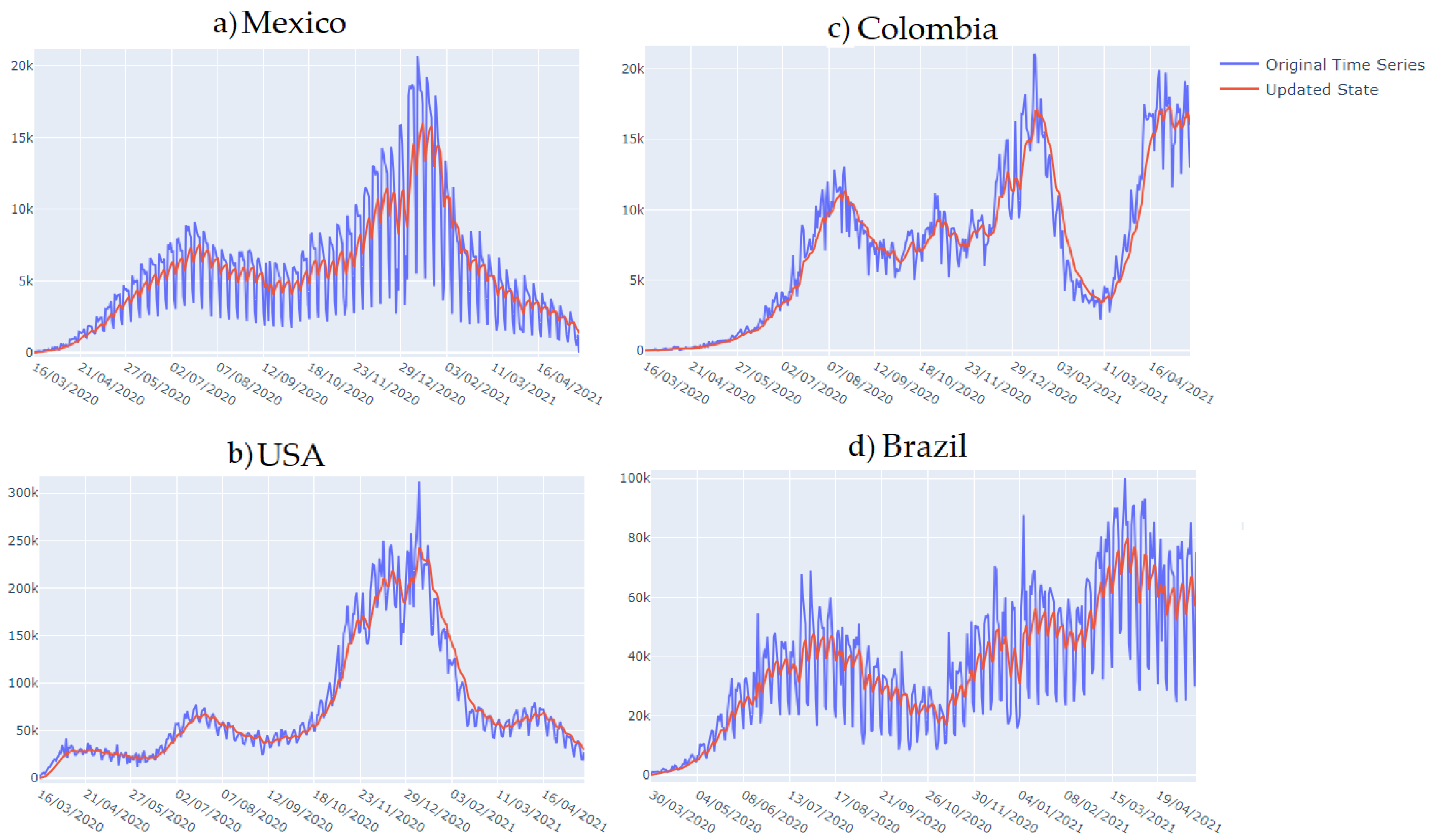
Figure 11 shows the time series filtered by KF for new cases of COVID-19 in (a) Mexico, (b) the USA, (c) Colombia, and (d) Brazil. During the DL training, normalized time series were used. These time series are shown in blue. The filtered time series were obtained with a one-dimensional KF, and they are shown in red.

The Kalman filter is commonly employed for one-step-ahead forecasting. However, in our application, we utilize it for time series smoothing. As the new data point arrives, the variance–covariance matrix is continuously updated, leading to a remarkably smoothed time series that primarily retains trend information. This approach is particularly effective for time series with low variability, as observed in the case of Mexico. Nevertheless, for time series with substantial variation, the resulting filtered series may also capture the trend and primary seasonalities, as seen in the remaining filtered countries in Figure 11.

5.2. Selecting the Best Forecast in the Validation Set

To determine the best forecast for the filtered time series, as previously described in Section 4.1, the configuration outlined in Table 2 is iterated $m$ times. The iteration with the best performance on the validation set is chosen to forecast the test set.

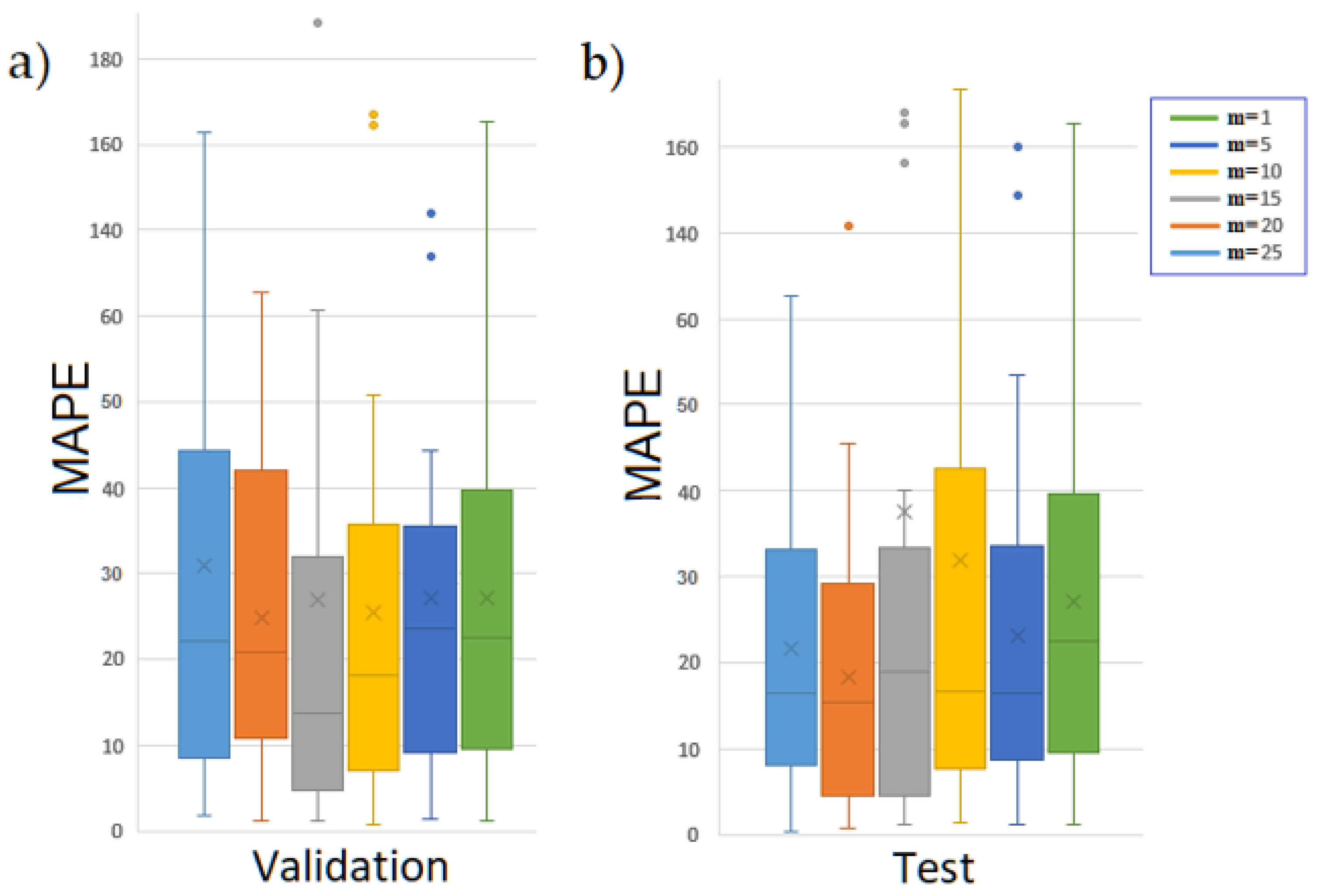
Figure 12 displays the forecast performance in a box plot measured with MAPE, wherein on the left-hand side is the validation, and on the right-hand side is the test. In this way, we show the central tendency and identify the outliers. The test forecast depends on selecting the best performance in the validation set through $m$ executions. We conducted a search ranging from $m$ = 1 to 25 to determine the optimal value. It is essential to note that, to prove the robustness of the approach, we ran the algorithm 30 times in order to adhere to the central limit theorem. For instance, for CNN with $m=5$, 5 training sessions are generated, and only the trained model with the best RMSE on the validation set is selected to make the test forecast. This search of $m$ is then repeated at least 30 times to generate a sufficient set of test forecasts that efficiently represent the performance of the search.

In the validation set, the occurrence of outliers decreases as $m$ increases. However, in the test forecast, the improvement in the average standard deviation does not consistently correspond to an increase of $m$. In our experiments, we observed that the optimal RMSE in both sets is achieved at $m=20$, which also corresponds to the highest number of forecasts near zero in MAPE. From another perspective, the uncertainty of the test forecast increases as HF grows. 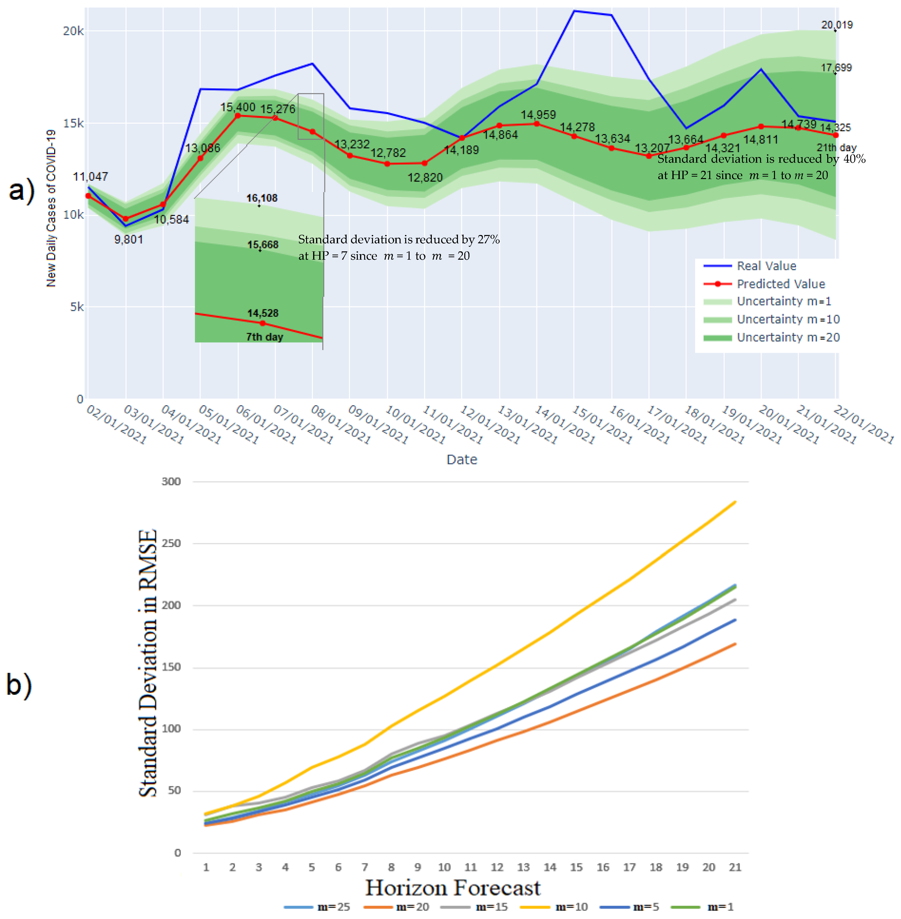Figure 13a displays a forecast of 21 days ahead, in which the real data are shown in the color blue; the mean of the forecast is shown in red, with markers; and the mean of the forecast is shown in text, where the variability of $m=$ 1, 10, and 20 is shown in green shadows to elucidated how it is reduced as $m$ increases. Figure 13b displays the evolution of the standard deviation in RMSE through the HF of the test forecast. As the HF is extended, there is great uncertainty in the forecast. Nevertheless, by selecting the execution with the best validation forecast (in this case, $m=20$ iterations), this uncertainty can be reduced by nearly 40% for 21 days and approximately 27% for 7 days of HF. We have noticed that, for $m>20$, the best forecast in validation does not necessarily correspond to the best forecast in the test set. The same steps are followed for forecasting the residual series in order to find the best possible result.

After obtaining the best validation forecast from $m=20$ executions, we conduct another search within these iterations to select the superior ${\widehat{e}}_k$ forecast, based on the configuration outlined in Table 3. Once the neural networks are trained for the filtered time series and the residual time series, we proceed with the test forecast by concatenating the training and validation sets. The final forecast is calculated as follows: ${\widehat{y}}_k^{test}={\widehat{w}}_k^{test}+{\widehat{e}}_k^{test}$, where ${\widehat{y}}_k^{test}$ is the final test forecast, ${\widehat{w}}_k^{test}$ is the filtered test forecast, and ${\widehat{e}}_k^{test}$ is the residual test forecast.

Table 4. Comparison of different combinations of the FMFRA-DL method to forecast new cases of COVID-19.

FILTER	${\widehat{\mathit{w}}}_{\mathit{K}}$	${\widehat{\mathit{e}}}_{\mathit{k}}$	USA			Brazil			Mexico			Colombia			Average
			MAPE	DA	RMSE	MAPE	DA	RMSE	MAPE	DA	RMSE	MAPE	DA	RMSE	MAPE	DA	RMSE
${SMA}_3$	LSTM	LSTM	23.32	40	63,543	18.59	85	11,153	55.84	75	9557	47.04	55	8521	36.2	63.75	23,194
		CNN	22.4	40	62,458	19.02	80	12,254	55.84	70	9458	45.45	55	8542	35.68	61.25	23,178
	CNN	LSTM	21.32	40	61,458	16.33	80	10,546	53.24	75	9245	37.84	55	8545	32.18	62.5	22,448
		CNN	20.04	45	60,840	15.42	80	9584	52.45	70	9345	38.45	60	8430	31.59	63.75	22,050
${SMA}_7$	LSTM	LSTM	9.45	50	28,864	10.34	85	5442	46.44	65	8228	29.51	65	5406	23.93	66.25	11,985
		CNN	9.48	50	29,485	10.36	85	5748	47.48	70	8345	30.21	65	5387	24.38	67.5	12,241
	CNN	LSTM	12.05	50	29,145	10.54	85	6548	43.48	75	8249	28.14	65	5347	23.55	68.75	12,322
		CNN	12.13	50	28,724	11.32	85	7542	43.24	70	8354	27.42	70	5345	23.53	68.75	12,491
KF	LSTM	LSTM	15.41	55	40,562	15.83	80	8982	50.57	80	8458	52.4	65	9057	33.55	70	16,765
		CNN	15.34	50	39,840	14.87	80	8578	48.52	75	8548	52.4	65	9154	32.78	67.5	16,530
	CNN	LSTM	15.78	50	40,874	12.48	80	8357	48.47	75	8874	49.45	65	9372	31.55	67.5	16,869
		CNN	16.01	55	42,265	13.34	80	8245	49.23	75	8947	48.07	65	9258	31.66	68.75	17,179

displays the performance of DL applied in this work, incorporating the filters and the residual analysis for the four aforementioned countries from March 2020 to July 2020. The twelve models are evaluated by MAPE, DA, and RMSE. We can observe, in the average column, that the combination of $SM{A}_7-LSTM-LSTM$ yields the best average RMSE, while $SM{A}_7-CNN-CNN$ exhibits the best average for DA and MAPE. This suggests that there is no definitive superiority between LSTM and CNN, but rather a filter-specific preference for this particular timeframe.

5.3. Comparison Results

The forecasting methods that combine various forecasting techniques are typically tailored to the specific characteristics of the time series. However, there is no universal superior forecasting technique. The FMFRA adjusts based on the validation performance, rather than being tied to the inherent time series characteristics. This approach offers increased flexibility and performance compared to powerful forecasting state-of-the-art ML methods. This methodology was tested in three time periods of the pandemic here.

5.3.1. Onset of the Pandemic

At the onset of the pandemic in countries across the American continent, the need for an effective forecasting method with limited training data was paramount. During the initial six months of the pandemic, spanning from 3 March 2020 to 5 September 2020, the available time series data did not provide sufficient information to generate reliable forecasts with an HF of 21 days. Nevertheless, the FMFRA methodology, which employs DL and SSA, demonstrated a superior performance, with the exception of the USA, as shown in

Table 5. Comparison of FMFRA vs. powerful state-of-the-art ML methods at the beginning of the pandemic.

Method	USA			Brazil			Mexico			Colombia			Average
	MAPE	DA	RMSE	MAPE	DA	RMSE	MAPE	DA	RMSE	MAPE	DA	RMSE	MAPE	DA	RMSE
SSA	15.7	75	6851	21.28	55	6906	21.29	85	1259	15.72	40	1253	18.49	63.75	4067
Kalantari [10]	29.26	75	11,973	33.47	75	8158	48.55	70	1728	12.52	55	1058	30.95	68.75	5729
${SMA}_7$-XGBoost-Res	11.66	75	5451	32.31	75	9497	29.97	80	1481	29.29	55	2156	26.38	71.25	4646
RFR	25.5	85	8008	47.03	60	10,417	33.46	90	1647	45.71	40	3273	37.93	68.78	5836
LR	6.97	80	6455	34.08	60	8695	21.67	80	1372	16.77	30	1444	19.87	62.5	4432
FMFRA	11.05	75	4877	20.15	55	6865	17.19	85	954	12.14	60	1048	12.63	68.75	3436
	SMA3-LSTM			SSA-Residuals			SMA3-LSTM			SSA-Residuals

.

FMFRA demonstrates superior performance compared to state-of-the-art methods. However, XGBoost and RFR show an acceptable DA. The filtering and residual analysis phases were applied, beating the other methods. Notably, when averaging the results from the four countries, FMFRA obtained the best performance, except in terms of the DA metric, where XGBoost performed better. However, it showed a notably poor MAPE metric. Notice that the best methods in this period were SSA and FMFRA regarding the best average results.

5.3.2. Peak of the Infections

Infectious disease time series tend to display more chaotic behavior as the number of infections increases. Understanding and accurately forecasting such intricate patterns became increasingly challenging as the pandemic progressed.

Table 6. FMFRA method results at the peak of infections of the pandemic (3 March 2020–18 November 2020).

Method	USA			Brazil			Mexico			Colombia			Average
	MAPE	DA	RMSE	MAPE	DA	RMSE	MAPE	DA	RMSE	MAPE	DA	RMSE	MAPE	DA	RMSE
SSA	17.14	60	46,572	29.65	65	11,045	29.65	65	6167	23.58	65	4641	23.61	61.25	17,102
XGBoost	20.15	50	53,961	31.81	80	15,041	31.81	80	6192	38.97	45	6970	31.35	62.5	20,541
RFR	15.47	40	43,731	38.49	65	10,202	38.49	65	6660	40.3	50	7316	29.13	53.75	16,977
LR	36.7	40	80,970	32.25	70	7196	32.25	70	7498	24.84	70	4809	26.87	62.5	25,118
FMFRA	9.45	50	2886	10.34	85	5442	24.29	70	6152	23.55	65	4633	16.92	67.5	11,279
	SMA7-LSTM			SMA7-LSTM			SSA-Residuals			SSA-Residuals

provides a comprehensive insight into the performance of the FMFRA method during the peak of infections in the American continent, spanning from 3 March 2020 to 18 November 2020. This critical period presented numerous challenges, as healthcare systems were strained under the weight of surging cases and governments implemented diverse measures in an attempt to curb the spread of COVID-19.

The DL methods often struggle to forecast infectious disease time series at infection peak periods. This is due to the challenge of distinguishing pronounced trends from noise. FMFRA demonstrated a superior performance, showcasing its adaptability and robustness, and addressing this by decomposing the time series with filters, aiding LSTM and CNN in trend capture. However, the results vary by country size and with larger populations, such as those in the USA and Brazil, facilitating trend modeling and yielding better LSTM and CNN results. The situation is different in countries with smaller populations, like Mexico and Colombia. By leveraging the decomposition and DL techniques, FMFRA has robust forecasting capabilities, even during the most demanding phases of a pandemic.

5.3.3. One Year into the Pandemic

From 3 March 2020 to 3 March 2021, covering the entirety of the annual seasonality cycle, LSTM and CNN showcased their enhanced ability to capture the trends in comparison with SSA. However, during the intervals marked by diminished volatility stemming from a decreased rate of new COVID-19 cases, SSA had a superior performance, as shown in

Table 7. $\mathrm{F}\mathrm{M}\mathrm{F}\mathrm{R}\mathrm{A}$ method results from one year into the pandemic (3 March 2020–18 November 2020).

Method	USA			Brazil			Mexico			Colombia			Average
	MAPE	DA	RMSE	MAPE	DA	RMSE	MAPE	DA	RMSE	MAPE	DA	RMSE	MAPE	DA	RMSE
SSA	22.07	85	8043	9.06	95	5344	57.33	95	1134	14.67	50	2846	25.16	81.25	4326
XGBoost	20.22	90	7253	17.83	80	13,784	89.42	80	1525	33	35	6138	40.12	71.25	7175
RFR	42.69	85	14,872	14.67	85	9205	68.32	100	1269	32.54	50	6021	39.56	80	7034
LR	40.06	85	14,510	13.33	80	8384	100.45	100	1578	19.12	55	3662	43.24	80	7541
FMFRA	19.11	90	6931	8.83	90	5328	54.82	95	1071	9.15	70	1734	22.98	86.25	3766
	SSA-Residuals			SSA-Residuals			SSA-Residuals			SSA-Residuals

.

6. Conclusions and Future Works

6.1. Conclusions

This work introduces the FMFRA method, a novel integration of deep learning models with SSA techniques, encompassing FMFRA-DL and FMFRA-SSA components. Unlike the traditional approaches that extract only the trend signal, FMFRA-DL divides the time series into filtered and residual signals, using filters to enhance the learning process. FMFRA-SSA, on the other hand, optimizes the configurations during the validation phase and improves the forecasts by predicting residual values.

This method has been tested on COVID-19 datasets from the USA, Brazil, Mexico, and Colombia. FMFRA demonstrated versatility across varying levels of noise and complexity in the time series, showcasing its unique filters and residual analysis approaches in dealing with the challenges of COVID-19 forecasting. The method’s robustness and adaptability to varied noise patterns and data imperfections represent a significant advancement in the field, providing a new avenue for accurate long-term forecasting in epidemiology.

One of the notable strengths of FMFRA lies in its data-driven approach, which is distinct from many of the conventional forecasting methods that depend on predefined mathematical models. FMFRA derives its predictive power from its ability to model and tune based on the data themselves, a feature that becomes especially valuable in situations where the availability of a precise mathematical model is limited or nonexistent. In DL, perturbations are commonly employed in the search for solutions to mitigate the issues of a vanishing gradient when using gradient descent. However, these perturbations are not always sufficient to circumvent local minima during the solution search process. Furthermore, FMFRA addresses these problems by selecting the optimal weight configuration from a set of high-quality solutions founded by $m$ executions. Notice that specialization on the validation set does not necessarily guarantee an improvement in the test forecast. In this study, a total of twenty executions were conducted to forecast the filtered time series and residual time series.

Although numerous forecasting methods frequently customize their strategies to suit the distinct features of a given time series, these attributes are prone to change over time, with recent events usually carrying greater relevance. This highlights why FMFRA, like other ML methods, places such importance on using validation performance as the primary factor in selecting models. While SSA residuals consistently yield satisfactory results, especially in the presence of noise, DL demonstrates the capacity to recognize and adjust to considerably more complex patterns, occasionally outperforming SSA residuals. This inherent adaptability in response to shifting data dynamics emerges as a prominent strength of FMFRA.

The inclusion of filtering and residual analysis phases in FMFRA enhances its forecasting capabilities in capturing trends and patterns. The filters that produced the best results in this forecasting method were ${SMA}_3$, ${SMA}_7$, and KF as a simple random walk. They surpassed the popular techniques for residual analysis, known as exponential smoothing and SARIMA. However, we recommend that they should be compared to other cases. These filtering methods effectively boost forecasting performance, especially when used in isolation from the residual analysis phase.

6.2. Future Works

An innovative aspect of FMFRA involves the decomposition of time series into filtered and residual components. This decomposition not only simplifies the fine-tuning of forecasting methods for specific time series, but also effectively addresses the issues related to noise. As a result, when forecasting new COVID-19 cases during the analyzed periods, SSA and DL emerged as the most effective options. This approach can be extended to other forecasting tasks, such as climate change prediction, where methods other than DL forecasting can be employed for the primary time series. For the residual time series, alternative forecasting methods can be utilized.

On the other hand, in the context of tracking new COVID-19 cases, the creation of a real-time forecasting module within FMFRA holds substantial potential for facilitating timely decision making for health authorities and policymakers. In terms of future work, an area of focus involves the exploration of an advanced KF that integrates a triple random walk model within the framework of H&W filtering. This enhancement would combine the benefits of the H&W method with the robustness to noise capabilities of KF, offering improved forecasting accuracy.