A Multi-Credit-Rating Migration Model with Asymmetric Migration Boundaries

Abstract

In this paper, we propose an extended credit migration model with asymmetric fixed boundaries and multiple ratings, for a more precise depiction of credit changes in the real world. A model with three ratings is established and analyzed as an example, and then the results are generalized to a general multirating form model. We prepare the model meaningfully by arranging the asymmetric boundaries in a suitable order. A PDE system problem is deduced, and the existence and uniqueness of the solution for the problem are obtained using PDE techniques, which further ensure the rationality of the model. Due to the flexible configuration of asymmetric boundaries, the multirating model has various types of structures in the buffer zones where the credit rating keeps its original state. For instance, the two buffers in the three-rating model may be separated, connected, or intersected, as presented in the numerical results for different boundary parameters.

1. Introduction

Credit risk refers to the possibility of credit-related events, which include defaults and migrations of credit ratings. After the financial crisis in 2008 and European debit crisis in 2010, credit migration risk has attracted more attention. Credit migration is a change in an issuer’s creditworthiness from one credit rating category to another. For example, at the onset of the European debit crisis, Greece’s sovereign credit rating was downgraded from an initial rating of “A” to “BBB” and subsequently, to “BB” or even lower. Investors holding Greek bonds experienced a decline in the value of their investments due to the increased credit risk and the credit ratings of other European countries were also affected due to broader concerns about the stability of the eurozone. Indeed, the credit migration risk has a great impact on the financial market, not only affecting confidence in the market but also affecting the value of financial products.

There have been some studies on the transformation of credit ratings, which can be traced back to the reduced form method. In detail, Jarrow, Lando and Turnbull [1] were the first to apply a Markov chain, and they adopted a transfer intensity matrix to capture the credit migration process. This reduced-form approach is developed naturally (see Arvanitis et al. [2], Hurd and Kuznetsov [3], Lando [4], Thomas et al. [5], Nguyen [6], Chen et al. [7] and so forth). The transfer intensity matrix is usually derived from general statistical data and mainly reflects the impact of macroeconomic factors on credit rating. However, the firm’s features, such as its financial status, play a key role in credit rating migration.

Liang et al. [8,9] took a firm’s asset value or capital structure as the major determinant of credit migration using the structural method. In detail, Liang and Zeng [8] built the first structural model to price bonds with credit migration, in which a given credit migration boundary divides the asset value into high- and low-rating regions. Further, Hu, Liang and Wu [9] governed the credit migration boundary via the liability–asset ratio rather than giving it directly, and they deduced a credit migration problem with a free boundary. However, setting a strict threshold in the structural model may lead to an infinite number of credit rating migrations under the assumption that the asset values follow a geometric Brownian motion. This is because Brownian motion crosses any level an infinite number of times in any time interval. Chen and Liang [10] and Liang and Lin [11] introduced a buffer zone to overcome this shortcoming in the free-boundary model [9] and the fixed-boundary model [8], respectively. That is, they set a pair of asymmetric thresholds for credit rating migration: one threshold for upgrades and the other slightly different threshold for downgrades. Compared to models with a strict threshold, those with asymmetric thresholds represent a significant improvement as they limit the frequency of credit rating transitions. All the models in [8,9,10,11] bifurcate credit ratings into two categories: high rating and low rating.

In reality, there are more than two ratings for firms’ credit. Rating agencies use a wide range of scales; for instance, Standard and Poor’s divides credit ratings into several letter grades ranging from “AAA” (the highest credit rating) to “C” (the lowest credit rating). For applications, it is necessary to consider structural models for credit migration in cases with multiple credit ratings. For the strict threshold model in [9], Wu and Liang [12] extended this to the case with three rating regions and suggested a general form for multi-credit-rating models. However, there has not yet been a multirating form proposed for the asymmetric threshold model. In fact, this form may have a more complex multirating structure as the downgrade threshold and upgrade threshold are different. To fill this research gap, we aim to define a well-posed multi-credit-rating model with asymmetric thresholds. We confirm the mathematical theory for the corresponding PDE problem to ensure the rationality of this kind of model and solve the problem in numerical schemes to show the different structures of models for different parameters of asymmetric boundaries. As a first attempt, we focus on the fixed-boundary problem in this paper.

Specifically, this article improved the model in [11] to the level of that with multiple credit ratings. First, we divide the firm’s value into low-, medium- and high-rating regions using two pairs of asymmetric boundaries within a proper order. Thus, a buffer zone is introduced between each pair of asymmetric boundaries, in which the credit rating maintains its status. Then, we derive a system of partial differential equations with several overlaps. For the existence of the solution, we construct convergence sequences by using a method of monotonic iteration. As a significant difference with [11], it is necessary to construct two sequences converging towards the solution on the intermediate-rating region (i.e., the medium rating in the three-rating model), for a complete iterative loop. And we prove the uniqueness of the solution by contradiction with more branches than [11]. Finally, the general multirating problem with asymmetric migration boundaries is obtained. This kind of model has more types of structures than the original multirating model in [12], which is mainly reflected in the aspect of buffers, due to the flexible asymmetric boundary settings. As far as we know, this is the first time that the asymmetric model with multiple ratings has been studied, which guarantees the model’s rationality and indicates its potential advantage in real-world settings.

The structure of this paper is as follows. In Section 2, the relevant literature is reviewed. In Section 3, we establish an asymmetric threshold model with three ratings, and derive a PDE system. In Section 4, by constructing monotonic sequences, we prove the existence of the solution to this problem. In Section 5, the uniqueness of the solution is confirmed via contradiction. Section 6 presents the numerical results for different parameters of asymmetric boundaries and conducts a real parameter calibration. Section 7 shows the form of general multirating models. Section 8 constitutes the conclusion and discussion.

2. Literature Review

The first structural model on credit risk could be traced back to Merton [13], which focuses on the default. In Merton’s model, the firm’s asset value was assumed to follow a geometric Brownian motion and a default would be triggered if the asset value fell below the debt at maturity. Thus, the corporate debt was a contingent claim of the asset value. Black and Cox [14] extended this model to allow the default to occur before maturity as long as the asset value dropped below a given threshold. For further research on structural models of defaults, see also Leland [15], Longstarff and Schwartz [16], Leland and Toft [17], Briys and deVarenne [18] and so forth. In addition to the default, the phenomenon of credit rating migration has also been analyzed, such as the stability and dependencies of rating transitions (Carty [19]; Nickell et al. [20]), non-Markov effects in rating drifts (Altman and Kao [21] and Lando and Skødeberg [22]), implied migration rates (Albanese and Chen [23]), etc. As for the valuation of credit migration risk, Liang et al. [8,9] pioneered the adoption of structured models, subsequently followed by a series of further studies, while the reduced-form model is another important method [2,3,4].

Under the framework of the structural model with a strict credit migration threshold, some studies have concentrated on model extension, theoretical exploration, empirical analysis and so forth. For instance, Wu et al. [24] extended the free-boundary model in [9] by permitting defaults to occur at any time up to maturity, while Li et al. [25] proved the convergence and error estimates of a finite difference scheme for this model. Lin and Liang [26] identified the credit migration boundaries empirically by pricing long-term corporate bonds in the U.S. financial market. And another crucial extension for applying the strict threshold model is to transition it from the simplicity of two-tiered ratings to a more general multirating scenario. Wu and Liang [12] extended the model in [9] to the multirating case, and Wang et al. [27] studied the asymptotic traveling-wave solution for the new model using an inductive method to overcome the multiplicity of free boundaries. Yin et al. [28] considered a multirating model with a stochastic interest rate based on the model in [29].

In the form of a structural model with a pair of different upgrade and downgrade thresholds, Chen and Liang [10] investigated the free-boundary problem, while Liang and Lin [11] explored the fixed-boundary one. Liang and Lin [30] presented more theoretical results primarily on the traveling-wave solution with a buffer zone. However, there is a research gap concerning the multirating scenarios for the asymmetric threshold model. It is imperative to proffer a general form of multirating asymmetric model and establish its well-posedness, which serves as the basis for further theoretical research and the practical applications of the model. In this paper, we begin to explore the asymmetric threshold model with multiple ratings, focusing on the fixed-boundary problem as the first step.

3. Model

3.1. Assumption

Let $(\Omega ,\mathcal{F},\mathcal{P})$ be a complete probability space. We assume that the firm issues one corporate bond, which is a contingent claim of its asset value and its credit rating in $(\Omega ,\mathcal{F},\mathcal{P})$.

Assumption 1

(Firm’s asset with credit rating migration). Let $S_t$ denote the firm’s asset value in the risk-neutral world. It satisfies

$$d{S}_t=\left\{\begin{array}{c}r{S}_{t}dt+{\sigma }_H{S}_{t}d{W}_t,in the high-rating region,\hfill \\ r{S}_{t}dt+{\sigma }_M{S}_{t}d{W}_t,in the medium-rating region,\hfill \\ r{S}_{t}dt+{\sigma }_L{S}_{t}d{W}_t,in the low-rating region.\hfill \end{array}\right.$$

where r is the risk-free interest rate, and positive constants

$${\sigma }_H<{\sigma }_M<{\sigma }_L$$

(1)

represent the volatility of the firm under the high, medium and low credit grades, respectively. $W_t$ is the standard Brownian motion which generates the filtration $\left\{{\mathcal{F}}_t\right\}$.

Remark 1.

It is reasonable to consider the asset process under the risk-neutral measure rather than the real-world measure, since we aim not to analyze the credit migration phenomenon for fitting the history data but to price a bond with credit migration for the valuation of credit migration risks. The probabilities of default based on this underlying process are forward-looking and point in time, although the credit rating are typically identified by rating agencies on the through-the-cycle methodology [31,32].

Remark 2.

It is natural to set (1) in Assumption 1, namely, that the volatility of a firm’s asset return in the higher-rating region is lower than the one in the lower-rating region.

Assumption 2

(Debt obligation). The firm issues a zero-coupon bond that has a face value of F. Denote by ${\Phi }_t$ the value of the bond at time t. At the maturity time T, the bond value is ${\Phi }_T=min\{S_T,F\}$.

Assumption 3

(Credit rating migration). Two pairs of asymmetric thresholds are introduced for the debt’s credit rating migration. The

$$S^{M_1}<S^L$$

(2)

are a pair of thresholds for downgrades and upgrades in the low- and medium-rating regions, and the

$$S^H<S^{M_2}$$

(3)

are the other pair of thresholds for downgrades and upgrades in the medium- and high-rating regions. To make the model meaningful, we assume that $S^{M_1}>F$, $S^L<S^{M_2}$ and $S^H>S^{M_1}$.

The changes in credit ratings are determined by the asset value $S_t$. Starting from time t, let ${\tau }_1,{\tau }_2,{\tau }_3,{\tau }_4$ denote the first moment when the firm’s credit is downgraded from a high-rating region, upgraded from a middle-rating region, downgraded from a middle-rating region and upgraded from a low-rating region, respectively. That is,

$$\begin{array}{cc}\hfill & {\tau }_1=inf\{\tau >t|S_{\tau }\le S^H,S_t>S^H\},\hfill \\ \hfill & {\tau }_2=inf\{\tau >t|S_{\tau }\ge S^{M_2},S^{M_1}<S_t<S^{M_2}\},\hfill \\ \hfill & {\tau }_3=inf\{\tau >t|S_{\tau }\le S^{M_1},S^{M_1}<S_t<S^{M_2}\},\hfill \\ \hfill & {\tau }_4=inf\{\tau >t|S_{\tau }\ge S^L,S_t<S^L\}.\hfill \end{array}$$

It is worth noting that credit migration occurs only between two adjacent ratings; for example, if $S_t$ leaves from the high rating or low rating, it can only enter the medium rating.

Remark 3.

The inequalities (2) and (3) ensure that there are buffers (the overlaps of adjacent rating regions) introduced for credit rating migrations. For example, the firm that has just upgraded to the middle rating will not immediately downgrade even if the asset value falls back below $S^L$, unless the asset value continues to fall to $S^{M_1}$. Therefore, the number of changes between every two adjacent ratings per unit time is limited.

Remark 4.

In Assumption 3, the parameters of thresholds $S^H$ and $S^L$ can theoretically be set into three cases: $S^H>S^L$, $S^H=S^L$ and $S^H<S^L$. In the first case, there are two separate overlapping areas, a low–medium overlap $S^{M_1}\le S\le S^L$ and a medium–high overlap $S^H\le S\le S^{M_2}$. In the second situation, these two overlapping areas are connected on $S=S^H\left(S^L\right)$. In the last case, these two overlapping regions have a common part, $S^H\le S\le S^L$. Thus, the buffer between the low and medium ratings and the buffer between the medium and high ratings have three kinds of positional relationships: separation, connection and intersection. However, the PDE problems derived from the above three cases are all in the same form, and a unified analysis method can be adopted. We only show the difference among these three situations in the numerical simulation.

3.2. Cash Flow

When discussing the cash flow of the bond, we consider that the bond is virtually terminated and substituted by a new one with a new credit rating if the credit rating migrates before the maturity T. Let ${\Phi }^H(s,t),{\Phi }^M(s,t)$ and ${\Phi }^L(s,t)$ denote the values of the bond in the high, medium and low grades, respectively. They can be represented by the conditional expectations of the following formulas:

$$\begin{array}{cc}\hfill {\Phi }^H(s,t)=& E[e^{-r(T-t)}min\{S_T,F\}·{\mathbf{1}}_{\{T\le {\tau }_1\}}\hfill \\ \hfill & +e^{-r({\tau }_1-t)}{\Phi }^M(S_{{\tau }_1},{\tau }_1)·{\mathbf{1}}_{\{{\tau }_1<T\}}|S_t=s>S^H],\hfill \end{array}$$

(4)

$$\begin{array}{cc}\hfill {\Phi }^M(s,t)=& E[e^{-r(T-t)}min\{S_T,F\}·{\mathbf{1}}_{\{T\le {\tau }_2\vee {\tau }_3\}}\hfill \\ \hfill & +e^{-r({\tau }_2-t)}{\Phi }^H(S_{{\tau }_2},{\tau }_2)·{\mathbf{1}}_{\{{\tau }_2<T\vee {\tau }_3\}}\hfill \\ \hfill & +e^{-r({\tau }_3-t)}{\Phi }^L(S_{{\tau }_3},{\tau }_3)·{\mathbf{1}}_{\{{\tau }_3<T\vee {\tau }_2\}}|S_t=s,S^{M_1}<s<S^{M_2}],\hfill \end{array}$$

(5)

$$\begin{array}{cc}\hfill {\Phi }^L(s,t)=& E[e^{-r(T-t)}min\{S_T,F\}·{\mathbf{1}}_{\{T\le {\tau }_4\}}\hfill \\ \hfill & +e^{-r({\tau }_4-t)}{\Phi }^M(S_{{\tau }_4},{\tau }_4)·{\mathbf{1}}_{\{{\tau }_4<T\}}|S_t=s<S^L],\hfill \end{array}$$

(6)

where ${\mathbf{1}}_{event}=1$ if the event happens and 0 otherwise.

3.3. PDE Problem

Using the Feynman–Kac formula (e.g., see [33]), it is not difficult to drive the partial differential equations that ${\Phi }^H,{\Phi }^M$ and ${\Phi }^L$ satisfy in their respective regions:

$$\begin{array}{cc}\hfill & \frac{\partial {\Phi }^H}{\partial t}+\frac{1}{2}{\sigma }_H^2{S}^2\frac{{\partial }^2{\Phi }^H}{\partial S^2}+rS\frac{\partial {\Phi }^H}{\partial S}-r{\Phi }^H=0,\mathrm{for}S>S^H,0<t<T,\hfill \\ \hfill & \frac{\partial {\Phi }^M}{\partial t}+\frac{1}{2}{\sigma }_M^2{S}^2\frac{{\partial }^2{\Phi }^M}{\partial S^2}+rS\frac{\partial {\Phi }^M}{\partial S}-r{\Phi }^M=0,\mathrm{for}{S}^{M_1}<S<S^{M_2},0<t<T,\hfill \\ \hfill & \frac{\partial {\Phi }^L}{\partial t}+\frac{1}{2}{\sigma }_L^2{S}^2\frac{{\partial }^2{\Phi }^L}{\partial S^2}+rS\frac{\partial {\Phi }^L}{\partial S}-r{\Phi }^L=0,\mathrm{for}0<S<S^L,0<t<T.\hfill \end{array}$$

with the following terminal condition:

$${\Phi }^H(S,T)={\Phi }^M(S,T)={\Phi }^L(S,T)=min\{S,F\}.$$

The Formulas (4)–(6) imply that the value of the bond is continuous when it passes the rating thresholds, i.e.,

$$\begin{array}{cc}\hfill & {\Phi }^H(S^H,t)={\Phi }^M(S^H,t),\hfill \\ \hfill & {\Phi }^M(S^{M_2},t)={\Phi }^H(S^{M_2},t),\hfill \\ \hfill & {\Phi }^M(S^{M_1},t)={\Phi }^L(S^{M_1},t),\hfill \\ \hfill & {\Phi }^L(S^L,t)={\Phi }^M(S^L,t).\hfill \end{array}$$

Thus, we get a complete PDE problem. Without a loss of generality, we assume that $F=1$. Using the standard change of variables $x=logS$ and renaming $T-t$ as t, from ${\Phi }^i(e^x,T-t)$, we obtain a function of the variables x and t, still denoted as ${\Phi }^i,i=H,M,L.$ They satisfy the equations and conditions as follows:

$$\left\{\begin{array}{cc}\frac{\partial {\Phi }^H}{\partial t}-\frac{1}{2}{\sigma }_H^2\frac{{\partial }^2{\Phi }^H}{\partial x^2}-(r-\frac{1}{2}{\sigma }_H^2)\frac{\partial {\Phi }^H}{\partial x}+r{\Phi }^H=0,\hfill & \mathrm{for}x>X^H,t>0,\hfill \\ {\Phi }^H(x,0)=min\{e^x,1\},\hfill & \mathrm{for}x>X^H,\hfill \\ {\Phi }^H(X^H,t)={\Phi }^M(X^H,t),\hfill & \mathrm{for}t>0,\hfill \\ \frac{\partial {\Phi }^M}{\partial t}-\frac{1}{2}{\sigma }_M^2\frac{{\partial }^2{\Phi }^M}{\partial x^2}-(r-\frac{1}{2}{\sigma }_M^2)\frac{\partial {\Phi }^M}{\partial x}+r{\Phi }^M=0,\hfill & \mathrm{for}{X}^{M_1}<x<X^{M_2},t>0,\hfill \\ {\Phi }^M(x,0)=min\{e^x,1\},\hfill & \mathrm{for}{X}^{M_1}<x<X^{M_2},\hfill \\ {\Phi }^M(X^{M_2},t)={\Phi }^H(X^{M_2},t),\hfill & \mathrm{for}t>0,\hfill \\ {\Phi }^M(X^{M_1},t)={\Phi }^L(X^{M_1},t),\hfill & \mathrm{for}t>0,\hfill \\ \frac{\partial {\Phi }^L}{\partial t}-\frac{1}{2}{\sigma }_L^2\frac{{\partial }^2{\Phi }^L}{\partial x^2}-(r-\frac{1}{2}{\sigma }_L^2)\frac{\partial {\Phi }^L}{\partial x}+r{\Phi }^L=0,\hfill & \mathrm{for}x<X^L,t>0,\hfill \\ {\Phi }^L(x,0)=min\{e^x,1\},\hfill & \mathrm{for}x<X^L,\hfill \\ {\Phi }^L(X^L,t)={\Phi }^M(X^L,t),\hfill & \mathrm{for}t>0.\hfill \end{array}\right.$$

(7)

where

$$\begin{array}{cc}\hfill & X^L=log{S}^L,\hfill \\ \hfill & X^{M_1}=log{S}^{M_1},X^{M_2}=log{S}^{M_2},\hfill \\ \hfill & X^H=log{S}^H.\hfill \end{array}$$

The meaning of all symbols in the PDE problem (7) is summarized in

Table 1. Symbols in the PDE problem (7).

${\mathbf{\Phi }}^{\mathit{i}}(\mathit{i}=\mathit{H},\mathit{M},\mathit{L})$	x	t	${\mathit{\sigma }}_{\mathit{i}}(\mathit{i}=\mathit{H},\mathit{M},\mathit{L})$	r	${\mathit{X}}^{\mathit{L}},{\mathit{X}}^{{\mathit{M}}_2}$	${\mathit{X}}^{{\mathit{M}}_1},{\mathit{X}}^{\mathit{H}}$
Bond value	Natural logarithm of asset value	Time to maturity	Volatility of asset return	Risk-free interest rate	Upgrade threshold	Downgrade threshold

.

4. Existence

In this section, we prove the existence of solutions to the PDE problem (7). It is not a general semi-unbounded problem or a Dirichlet problem, since the value of the solution on the boundaries is not given. We use a monotonic iterative method, which is a generalization from [10,11]. In detail, starting from ${\Phi }_0^L(X^L,t)\equiv 1$ and ${\Phi }_0^{M,1}(X^{M_2},t)\equiv 1$, we successively construct the sequences ${\{{\Phi }_k^L,{\Phi }_k^{M,1},{\Phi }_k^{M,2},{\Phi }_k^H\}}_{k=0}^{\infty }$ which are decreasing with k. Sending $k\to \infty$, we obtain the limit as a solution.

4.1. Monotonic Sequences

We first define the sequences via induction and then show that the sequences are monotonic. Define the operator ${\mathcal{L}}^i=\frac{\partial }{\partial t}-\frac{1}{2}{{\sigma }_i}^2\frac{{\partial }^2}{\partial x^2}-(r-\frac{1}{2}{{\sigma }_i}^2)\frac{\partial }{\partial x}+r$, $i=H,M,L$ and the domains $Q^L=(-\infty ,X^L)\times (0,+\infty )$, $Q^M=(X^{M_1},X^{M_2})\times (0,+\infty )$ and $Q^H=(X^H,+\infty )\times (0,+\infty )$. Suppose $k\ge 0$ is an integer.

Step 1.

Define ${\Phi }_0^L(x,t)$ as the solution of

$$\left\{\begin{array}{cc}{\mathcal{L}}^L{\Phi }_0^L=0,\hfill & \mathrm{for}x<X^L,t>0,\hfill \\ {\Phi }_0^L(x,0)=min\{e^x,1\},\hfill & \mathrm{for}x<X^L,\hfill \\ {\Phi }_0^L(X^L,t)=1,\hfill & \mathrm{for}t>0.\hfill \end{array}\right.$$

(8)

This is a general semi-unbounded problem for a diffusion equation in $Q^L$, and the solution satisfies the compatibility conditions. It has a closed-form solution and ${\Phi }_0^L(x,t)\in C^{\infty }(\overline{Q^L}\setminus (0,0))$.

Step 2.

Define ${\Phi }_0^{M,1}(x,t)$ as the solution of

$$\left\{\begin{array}{cc}{\mathcal{L}}^M{\Phi }_0^{M,1}=0,\hfill & \mathrm{for}{X}^{M_1}<x<X^{M_2},t>0,\hfill \\ {\Phi }_0^{M,1}(x,0)=min\{e^x,1\},\hfill & \mathrm{for}{X}^{M_1}<x<X^{M_2},\hfill \\ {\Phi }_0^{M,1}(X^{M_1},t)={\Phi }_0^L(X^{M_1},t),\hfill & \mathrm{for}t>0,\hfill \\ {\Phi }_0^{M,1}(X^{M_2},t)=1,\hfill & \mathrm{for}t>0,\hfill \end{array}\right.$$

(9)

Since ${\Phi }_0^L$ is solved, the value of ${\Phi }_0^{M,1}$ on the boundary is already known. Thus, such a Dirichlet problem in $Q^M$ generates a solution ${\Phi }_0^{M,1}(x,t)\in C^{\infty }\left(\overline{Q^M}\right)$.

Step 3.

Assuming ${\Phi }_{k-1}^L,{\Phi }_{k-1}^{M,1},k\ge 1$ are known, ${\Phi }_{k-1}^H,{\Phi }_{k-1}^{M,2},{\Phi }_k^L,{\Phi }_k^{M,1}$ could be defined via induction.

${\Phi }_{k-1}^H$ is defined as the solution of

$$\left\{\begin{array}{cc}{\mathcal{L}}^H{\Phi }_{k-1}^H=0,\hfill & \mathrm{for}x>X^H,t>0,\hfill \\ {\Phi }_{k-1}^H(x,0)=min\{e^x,1\},\hfill & \mathrm{for}x>X^H,\hfill \\ {\Phi }_{k-1}^H(X^H,t)={\Phi }_{k-1}^{M,1}(X^H,t),\hfill & \mathrm{for}t>0.\hfill \end{array}\right.$$

${\Phi }_{k-1}^{M,2}$ is defined as the solution of

$$\left\{\begin{array}{cc}{\mathcal{L}}^M{\Phi }_{k-1}^{M,2}=0,\hfill & \mathrm{for}{X}^{M_1}<x<X^{M_2},t>0,\hfill \\ {\Phi }_{k-1}^{M,2}(x,0)=min\{e^x,1\},\hfill & \mathrm{for}{X}^{M_1}<x<X^{M_2},\hfill \\ {\Phi }_{k-1}^{M,2}(X^{M_1},t)={\Phi }_{k-1}^{M,1}(X^{M_1},t),\hfill & \mathrm{for}t>0,\hfill \\ {\Phi }_{k-1}^{M,2}(X^{M_2},t)={\Phi }_{k-1}^H(X^{M_2},t),\hfill & \mathrm{for}t>0.\hfill \end{array}\right.$$

${\Phi }_k^L$ is defined as the solution of

$$\left\{\begin{array}{cc}{\mathcal{L}}^L{\Phi }_k^L=0,\hfill & \mathrm{for}x<X^L,t>0,\hfill \\ {\Phi }_k^L(x,0)=min\{e^x,1\},\hfill & \mathrm{for}x<X^L,\hfill \\ {\Phi }_k^L(X^L,t)={\Phi }_{k-1}^{M,2}(X^L,t),\hfill & \mathrm{for}t>0.\hfill \end{array}\right.$$

${\Phi }_k^{M,1}$ is defined as the solution of

$$\left\{\begin{array}{cc}{\mathcal{L}}^M{\Phi }_k^{M,1}=0,\hfill & \mathrm{for}{X}^{M_1}<x<X^{M_2},t>0,\hfill \\ {\Phi }_k^{M,1}(x,0)=min\{e^x,1\},\hfill & \mathrm{for}{X}^{M_1}<x<X^{M_2},\hfill \\ {\Phi }_k^{M,1}(X^{M_1},t)={\Phi }_k^L(X^{M_1},t),\hfill & \mathrm{for}t>0,\hfill \\ {\Phi }_k^{M,1}(X^{M_2},t)={\Phi }_{k-1}^{M,2}(X^{M_2},t),\hfill & \mathrm{for}t>0.\hfill \end{array}\right.$$

This completes the construction of the sequences ${\{{\Phi }_k^L,{\Phi }_k^{M,1},{\Phi }_k^H,{\Phi }_k^{M,2}\}}_{k=0}^{\infty }$ that satisfy

$$\begin{array}{cc}\hfill & {\Phi }_k^L(x,t)\in C^{\infty }(\overline{Q^L}\setminus (0,0)),{\Phi }_k^H(x,t)\in C^{\infty }\left(\overline{Q^H}\right),\hfill \\ \hfill & {\Phi }_k^{M,1}(x,t),{\Phi }_k^{M,2}(x,t)\in C^{\infty }\left(\overline{Q^M}\right),\mathrm{for}\mathrm{all}k\ge 0.\hfill \end{array}$$

Remark 5.

It is necessary to build two sequences ${\Phi }_k^{M,1}$ and ${\Phi }_k^{M,2}$ towards ${\Phi }^M$ to form an iterative loop. The establishment of the existence of solutions to the general multirating problem follows the same rule; two iterative sequences need to be constructed for the solution function on the intermediate-rating region.

Lemma 1.

The sequences ${\{{\Phi }_k^L,{\Phi }_k^{M,1},{\Phi }_k^H,{\Phi }_k^{M,2}\}}_{k=0}^{\infty }$ are monotonically decreasing with a lower bound; in fact, for each $k\ge 0$,

$$\begin{array}{cc}\hfill & 0\le {\Phi }_{k+1}^H\le {\Phi }_k^H,\mathrm{in}\overline{Q^H},\hfill \\ \hfill & 0\le {\Phi }_{k+1}^L\le {\Phi }_k^L,\mathrm{in}\overline{Q^L}.\hfill \\ \hfill & 0\le {\Phi }_{k+1}^{M,2}\le {\Phi }_{k+1}^{M,1}\le {\Phi }_k^{M,2}\le {\Phi }_k^{M,1},\mathrm{in}\overline{Q^M}.\hfill \end{array}$$

Consequently, for each $(x,t)\in Q^H,Q^M$ or $Q^L$, there are the limits

$$\begin{array}{cc}\hfill & {\Phi }^H(x,t)=\underset{k\to \infty }{lim}{\Phi }_k^H(x,t),{\Phi }^L(x,t)=\underset{k\to \infty }{lim}{\Phi }_k^L(x,t)\hfill \\ \hfill & {\Phi }^M(x,t)=\underset{k\to \infty }{lim}{\Phi }_k^{M,2}(x,t)=\underset{k\to \infty }{lim}{\Phi }_k^{M,1}(x,t)\hfill \end{array}$$

(10)

Proof. 

The main idea of the proof is to take the maximum principle and comparison principle (e.g., see [34]) repeatedly.

First, we show ${\Phi }_0^{M,2}<{\Phi }_0^{M,1}$ in $Q^M$ and ${\Phi }_1^L<{\Phi }_0^L$ in $Q^L$. For a semi-unbounded problem (8), using the maximum principle gives ${\Phi }_0^L(x,t)<1$. Thus, ${\Phi }_0^{M,1}(X^{M_1},t)={\Phi }_0^L(X^{M_1},t)<1$ for $t>0$. For the Dirichlet problem (9), using the maximum principle, we obtain

$${\Phi }_0^{M,1}(x,t)<1,\forall (x,t)\in Q^M.$$

Therefore, ${\Phi }_0^H(X^H,t)={\Phi }_0^{M,1}(X^H,t)<1$ for $t>0$. It follows that ${\Phi }_0^H(x,t)<1$ in $Q^H$ according to the maximum principle. Given that ${\Phi }_0^{M,2}(X^{M_2},t)={\Phi }_0^H(X^{M_2},t)$, we have ${\Phi }_0^{M,2}(X^{M_2},t)<1$ for $t>0$. Noting that ${\Phi }_0^{M,1}(X^{M_2},t)=1$ and ${\Phi }_0^{M,2}(X^{M_1},t)={\Phi }_0^{M,1}(X^{M_1},t)$, using the comparison principle, we find

$${\Phi }_0^{M,2}(x,t)<{\Phi }_0^{M,1}(x,t),\forall (x,t)\in Q^M.$$

(11)

Further, ${\Phi }_0^{M,2}<1$ in $Q^M$. Hence, ${\Phi }_1^L(X^L,t)={\Phi }_0^{M,2}(X^L,t)<1$. Combining with ${\Phi }_0^L(X^L,t)=1$ yields

$${\Phi }_1^L(x,t)<{\Phi }_0^L(x,t),\forall (x,t)\in Q^L.$$

(12)

Then, we make an inductive assumption that ${\Phi }_{k-1}^{M,2}<{\Phi }_{k-1}^{M,1}$ in $Q^M$,${\Phi }_k^L<{\Phi }_{k-1}^L$ in $Q^L,k\ge 1$.

On account of the iterative relationships ${\Phi }_k^{M,1}(X^{M_1},t)={\Phi }_k^L(X^{M_1},t)$ and ${\Phi }_{k-1}^{M,2}(X^{M_1},t)={\Phi }_{k-1}^{M,1}(X^{M_1},t)={\Phi }_{k-1}^L(X^{M_1},t)$, we obtain ${\Phi }_k^{M,1}(X^{M_1},t)<{\Phi }_{k-1}^{M,2}(X^{M_1},t)$ for $t>0$. And considering that ${\Phi }_k^{M,1}(X^{M_2},t)={\Phi }_{k-1}^{M,2}(X^{M_2},t)$, using the comparison principle, we obtain

$${\Phi }_k^{M,1}(x,t)<{\Phi }_{k-1}^{M,2}(x,t),\forall (x,t)\in Q^M.$$

(13)

Combined with ${\Phi }_{k-1}^{M,2}<{\Phi }_{k-1}^{M,1}$ in $Q^M$, we have ${\Phi }_k^{M,1}<{\Phi }_{k-1}^{M,1}$ in $Q^M$.

Also, the iterative conditions ${\Phi }_k^H(X^H,t)={\Phi }_k^{M,1}(X^H,t)$ and ${\Phi }_{k-1}^H(X^H,t)={\Phi }_{k-1}^{M,1}(X^H,t)$ imply ${\Phi }_k^H(X^H,t)<{\Phi }_{k-1}^H(X^H,t)$. Appling the comparison principle shows that

$${\Phi }_k^H(x,t)<{\Phi }_k^H(x,t),\forall (x,t)\in Q^H.$$

(14)

From this, we deduce that

$$\begin{array}{cc}\hfill {\Phi }_k^{M,2}(X^{M_2},t)={\Phi }_k^H(X^{M_2},t)& <{\Phi }_{k-1}^H(X^{M_2},t)\hfill \\ \hfill & ={\Phi }_{k-1}^{M,2}(X^{M_2},t)={\Phi }_k^{M,1}(X^{M_2},t).\hfill \end{array}$$

Combined with ${\Phi }_k^{M,2}(X^{M_1},t)={\Phi }_k^{M,1}(X^{M_1},t)$, it follows that

$${\Phi }_k^{M,2}(x,t)<{\Phi }_k^{M,1}(x,t),\forall (x,t)\in Q^M.$$

(15)

Noting (13), we conclude that ${\Phi }_k^{M,2}<{\Phi }_{k-1}^{M,2}$ in $Q^M$.

We thus obtain

$$\begin{array}{c}\hfill {\Phi }_{k+1}^L(X^L,t)={\Phi }_k^{M,2}(X^L,t)<{\Phi }_{k-1}^{M,2}(X^L,t)={\Phi }_k^L(X^L,t).\end{array}$$

According to the comparison principle,

$${\Phi }_{k+1}^L(x,t)<{\Phi }_k^L(x,t),\forall (x,t)\in Q^L.$$

(16)

From Equations (13)–(16), we can see that the induction argument for the monotonicity of the sequences is completed.

Similarly, via induction, we can derive that for each $k\ge 0$, ${\Phi }_k^L,{\Phi }_k^{M_1},{\Phi }_k^{M,2},{\Phi }_k^H\ge 0$. □

Lemma 2.

${\Phi }^H(x,t),{\Phi }^M(x,t)$ and ${\Phi }^L(x,t)$ defined by (10) form a solution for the PDE problem (7).

Proof. 

I. ${\mathcal{L}}^H{\Phi }^H=0$ in $Q^H$, ${\mathcal{L}}^M{\Phi }^M=0$ in $Q^M$, and ${\mathcal{L}}^L{\Phi }^L=0$ in $Q^L$.

Based on interior estimates of parabolic differential equations, it is easy to obtain that any finite derivative of ${\Phi }_k^i$ is uniformly bounded for $k\ge 0$ in any interior neighborhood of $(x,t)\in Q^i$ for $i=H,M,L$. Thus, we can deduce that ${\Phi }^i,i=H,M,L$ is infinitely differentiable within its region and satisfies the corresponding equation.

II. ${\Phi }^H,{\Phi }^M$ and ${\Phi }^L$ satisfy the initial and boundary conditions.

For any $k\ge 0$, ${\Phi }_k^H(x,0)={\Phi }_k^M(x,0)={\Phi }_k^L(x,0)=min\{e^x,1\}$, hence it is obvious that

$${\Phi }^H(x,0)={\Phi }^M(x,0)={\Phi }^L(x,0)=min\{e^x,1\}.$$

Since

$$\begin{array}{cc}\hfill & {\Phi }_{k-1}^H(X^H,t)={\Phi }_{k-1}^{M,1}(X^H,t),{\Phi }_{k-1}^{M,2}(X^{M_2},t)={\Phi }_{k-1}^H(X^{M_2},t),\hfill \\ \hfill & {\Phi }_k^L(X^L,t)={\Phi }_{k-1}^{M,2}(X^L,t),{\Phi }_k^{M,1}(X^{M_1},t)={\Phi }_k^L(X^{M_1},t),\hfill \end{array}$$

for all $k\ge 1$, as $k\to +\infty$, we obtain

$$\begin{array}{cc}\hfill & {\Phi }^H(X^H,t)={\Phi }^M(X^H,t),{\Phi }^M(X^{M_2},t)={\Phi }^H(X^{M_2},t),\hfill \\ \hfill & {\Phi }^L(X^L,t)={\Phi }^M(X^L,t),{\Phi }^M(X^{M_1},t)={\Phi }^L(X^{M_1},t).\hfill \end{array}$$

□

4.2. Existence

Lemma 2 gives the following existence result:

Theorem 1

(Existence). Problem (7) admits a solution $({\Phi }^L,{\Phi }^M,{\Phi }^H)$ that satisfies

$${\Phi }^L(x,t)\in C^{\infty }(\overline{Q^L}\setminus (0,0)),{\Phi }^M(x,t)\in C^{\infty }\left(\overline{Q^M}\right),{\Phi }^H(x,t)\in C^{\infty }\left(\overline{Q^H}\right).$$

5. Uniqueness

We use the maximum principle to prove the uniqueness of the solution of problem (7). Since the asymmetric boundary of each region is inside another region, the solution of each region cannot obtain the maximum or minimum value on the boundary.

Theorem 2

(Uniqueness). The solution of problem (7) is unique.

Proof. 

It suffices to show that the following equation has solutions only for zero functions.

$$\left\{\begin{array}{cc}{\mathcal{L}}^H{\Phi }^H=0,\hfill & \mathrm{for}x>X^H,t>0,\hfill \\ {\Phi }^H(x,0)=0,\hfill & \mathrm{for}x>X^H,\hfill \\ {\Phi }^H(X^H,t)={\Phi }^M(X^H,t),\hfill & \mathrm{for}t>0,\hfill \\ {\mathcal{L}}^M{\Phi }^M=0,\hfill & \mathrm{for}{X}^{M_1}<x<X^{M_2},t>0,\hfill \\ {\Phi }^M(x,0)=0,\hfill & \mathrm{for}{X}^{M_1}<x<X^{M_2},\hfill \\ {\Phi }^M(X^{M_2},t)={\Phi }^H(X^{M_2},t),\hfill & \mathrm{for}t>0,\hfill \\ {\Phi }^M(X^{M_1},t)={\Phi }^L(X^{M_1},t),\hfill & \mathrm{for}t>0,\hfill \\ {\mathcal{L}}^L{\Phi }^L=0,\hfill & \mathrm{for}x<X^L,t>0,\hfill \\ {\Phi }^L(x,0)=0,\hfill & \mathrm{for}x<X^L,\hfill \\ {\Phi }^L(X^L,t)={\Phi }^M(X^L,t),\hfill & \mathrm{for}t>0.\hfill \end{array}\right.$$

(17)

We first show that ${\Phi }^L\le 0$ in $Q^L$. If not, there is a point which is denoted by $(x_0,t_0)$ in $Q^L$ such that ${\Phi }^L(x_0,t_0)>0$. According to the maximum principle, the maximum value of ${\Phi }^L$ in $\overline{Q^L}$, represented by ${\Phi }_{max}^L$, must be taken at the boundary. Since ${\Phi }^L\equiv 0$ at $t=0$, there must be a point on $x=X^L$, denoted by $(X^L,t_1),t_1>0$, such that ${\Phi }^L(X^L,t_1)={\Phi }_{max}^L$.

Clearly, ${\Phi }^M(X^L,t_1)={\Phi }^L(X^L,t_1)>0$. From the maximum principle, the maximum value of ${\Phi }^M$ in $\overline{Q^M}$, represented by ${\Phi }_{max}^M$, must be taken at the boundary. Since ${\Phi }^M\equiv 0$ at $t=0$, there must be a point on $x=X^{M_1}$, denoted by $(X^{M_1},t_2),t_2>0$, such that ${\Phi }^M(X^{M_1},t_2)={\Phi }_{max}^M$, or a point on $x=X^{M_2}$, denoted by $(X^{M_2},t_3),t_3>0$, such that ${\Phi }^M(X^{M_2},t_3)={\Phi }_{max}^M$.

If the former holds, then

$${\Phi }^M(X^{M_1},t_2)>{\Phi }^M(X^L,t_1)={\Phi }^L(X^L,t_1).$$

(18)

Since $(X^{M_1},t_2)\in Q^L$, we also see that

$${\Phi }^L(X^L,t_1)>{\Phi }^L(X^{M_1},t_2)={\Phi }^M(X^{M_1},t_2),$$

(19)

contrary to (18).

If the latter is true, then ${\Phi }^H(X^{M_2},t_3)={\Phi }^M(X^{M_2},t_3)>0$. Using the maximum principle, the maximum value of ${\Phi }^H$ in $\overline{Q^H}$, represented as ${\Phi }_{max}^H$, must be taken at the boundary. Since ${\Phi }^H\equiv 0$ at $t=0$, there exists a point on $x=X^H$, denoted by $(X^H,t_4),t_4>0$, such that ${\Phi }^H(X^H,t_4)={\Phi }_{max}^H$. It follows that

$${\Phi }^H(X^H,t_4)>{\Phi }^H(X^{M_2},t_3)={\Phi }^M(X^{M_2},t_3).$$

(20)

As $(X^H,t_4)\in Q^M$, we have

$${\Phi }^M(X^{M_2},t_3)>{\Phi }^M(X^H,t_4)={\Phi }^H(X^H,t_4),$$

(21)

which is a contradiction.

Next, we can prove that ${\Phi }^L\ge 0$ in $Q^L$ in the same manner. It follows immediately that ${\Phi }^L\equiv 0$ in $Q^L$.

Similarly, we have ${\Phi }^M\equiv 0$ in $Q^M$ and ${\Phi }^H\equiv 0$ in $Q^H$. □

6. Numerical Results

We used an explicit difference scheme to calculate ${\Phi }^i(x,t),i=H,M,L$ and present the results in figures. The parameters we chose as examples are listed in the figure captions.

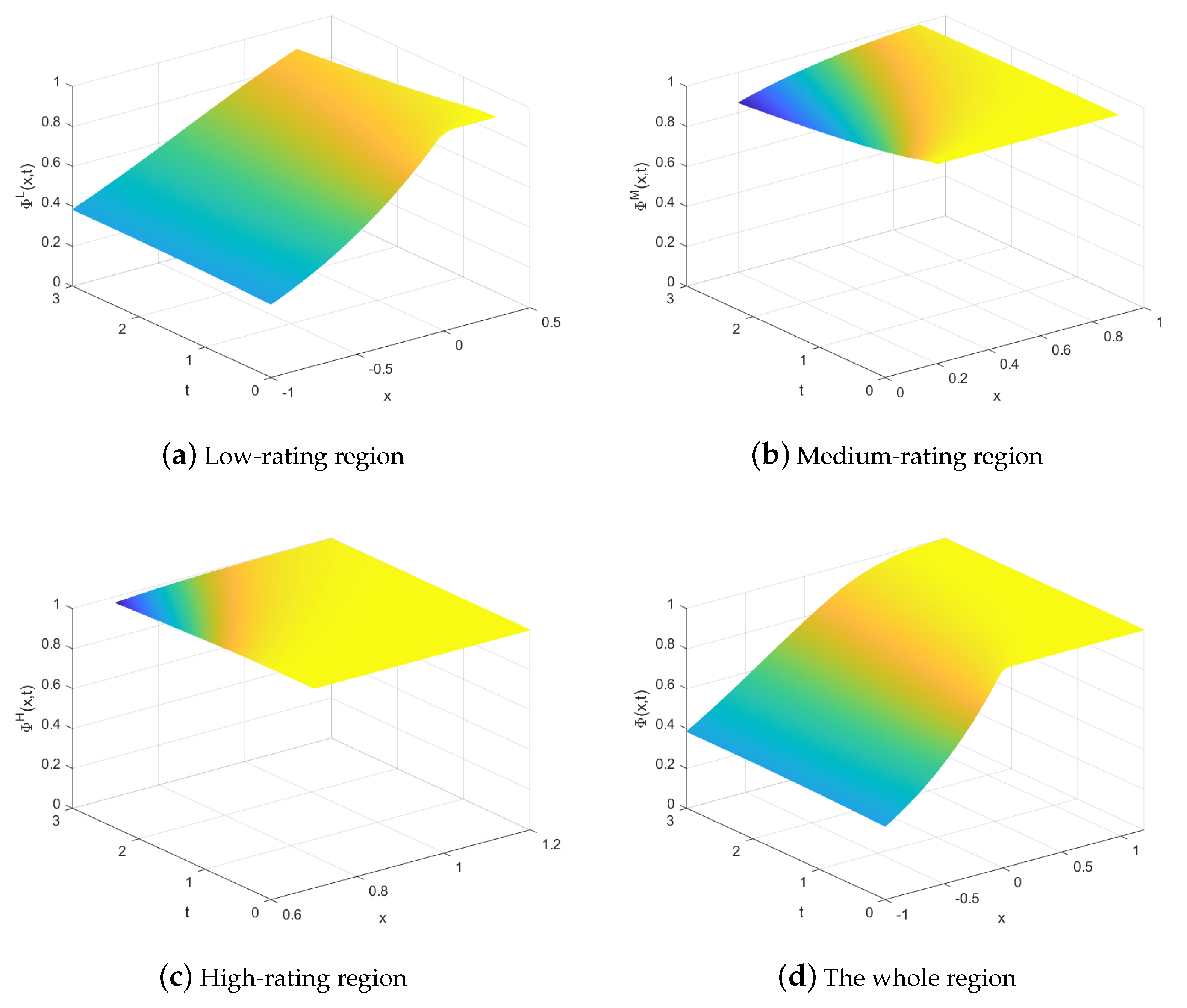
Figure 1 shows the bond value functions on different rating regions. Figure 1a–c depict the function images on the low-, medium- and high-rating regions that correspond to the domains $x\le X^L$, $X^{M_1}\le x\le X^{M_2}$ and $x\ge X^H$, respectively. The function image on the lower-rating region exhibits greater variation with respect to x, which implies that lower-grade bonds are more affected by the asset value. Note that Figure 1d displays the overall shape of the function graph across the entire region. In fact, there is an overlapping area between every two adjacent rating regions, forming a buffer zone for credit rating migrations where the credit rating maintains its original status. The overlap of the low-rating and medium-rating regions is confined in the range of $X^{M_1}\le x\le X^L$, while that of the medium-rating and high-rating regions is restricted within the interval $X^H\le x\le X^{M_2}$. In these overlaps, the graphs of the functions effectively consist of two layers, and the differences between these layers are depicted in Figure 2.

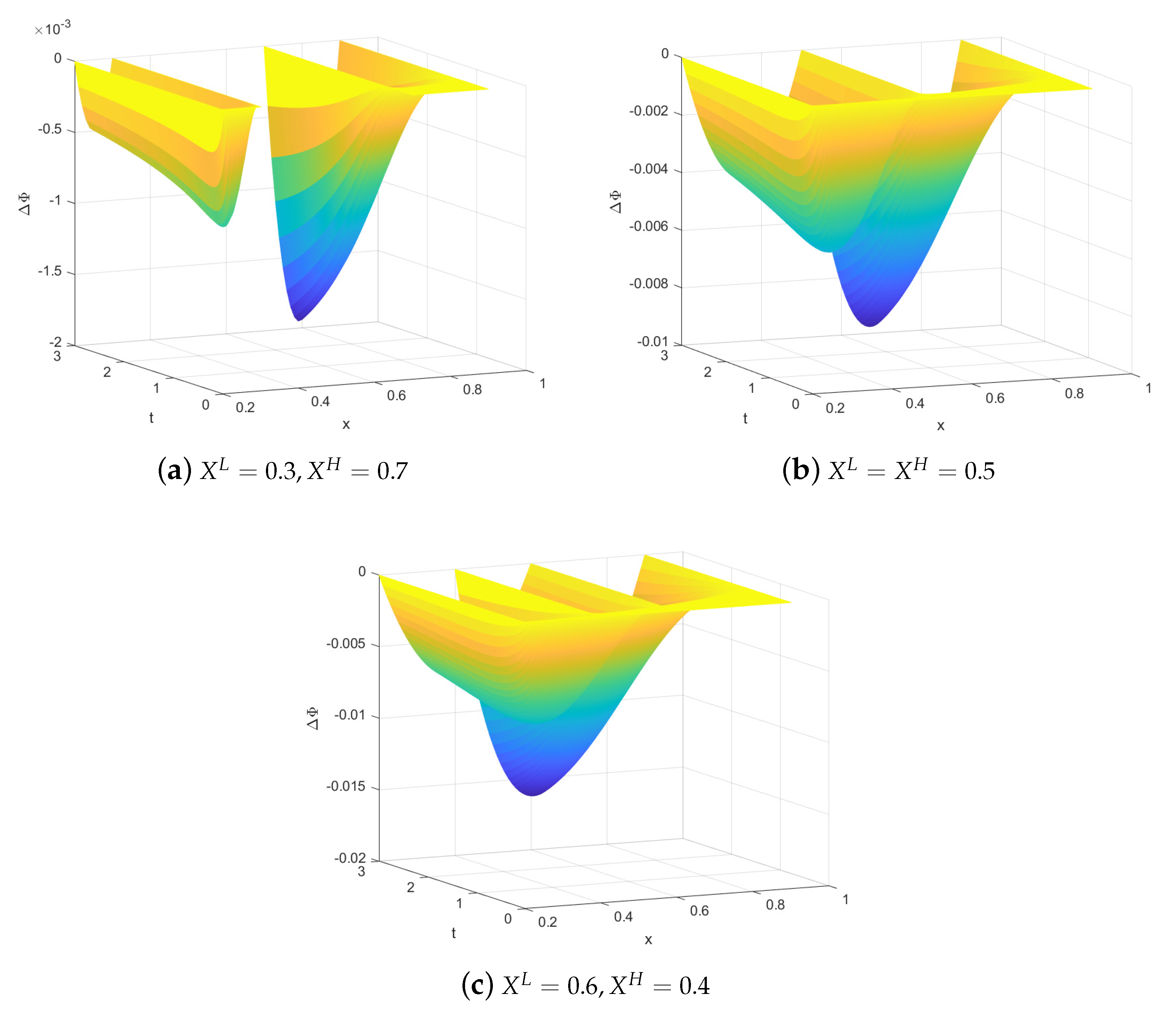
We can see the differences are negative, except at zero on the boundaries in Figure 2, which means that the price of higher-grade bonds exceeds that of lower-grade bonds in the buffer zone, although the gap is not huge. Figure 2a–c were prepared based on three groups of different asymmetric boundary parameters, respectively. From Figure 2a with $X^L=0.3,X^H=0.7$, the low–medium overlap and the medium–high overlap are separate. In Figure 2b with $X^L=X^H=0.5$, the two overlaps are connected on $x=0.5(x=X^H\left(X^L\right))$. In Figure 2c with $X^L=0.6,X^H=0.4$, the function images on the two overlaps are crossed together. Indeed, the two overlaps have a common part, the low–medium–high overlap $0.4\le x\le 0.6(X^H\le x\le X^L)$, where the credit rating of bonds may fall into any of the three categories: low, medium or high. Conclusively, each set of parameters represents a kind of theoretically meaningful configuration of asymmetric boundaries: $X^H>X^L$ , $X^H=X^L$ or $X^H<X^L$. The flexibility in boundary settings leads to various structures in the buffer zones for the multirating model with asymmetric boundaries, which contributes to identifying different types of credit migration phenomena.

The above numerical results are calculated by employing example parameters. We now explain how to carry out a real parameter calibration in the model by taking the Walt Disney Company (DIS) as an example. The calibration method we use is similar to that of Liang and Lin [11], albeit more intricate, as we need to calibrate more migration boundary parameters and volatility parameters than the two-rating case.

We analyze the DIS from 15 October 2001 to 12 March 2019. During this interval, the DIS underwent four credit rating migrations on the dates highlighted in

Table 2. Credit ratings for DIS.

Date	Rating	Type
⋯	⋯	-
27 February 1996	A	Medium rating
15 October 2001	A−	Low rating
4 October 2002	BBB+	Low rating
2 June 2005	A−	Low rating
5 October 2007	A	Medium rating
3 May 2017	A+	High rating
12 March 2019	A	Medium rating
⋯	⋯	-

Source: Standard & Poor’s.

, considering “A−” and “BBB+” as the low rating, “A” as the medium rating and “A+” as the high rating. The thresholds for downgrades and upgrades, $S^{M_1}$, $S^L$, $S^H$ and $S^{M_2}$, are the asset values at the time when the credit rating changes, which can be approximated by the sum of the market capitalization and the book value of the total liabilities. The face value of debt F is represented by the average of total liabilities reported in the balanced sheet during this interval. Thus, we can obtain the transformed thresholds, $X^{M_1}$, $X^L$, $X^H$ and $X^{M_2}$, by $x=log(S/F)$. The asset return volatility in different ratings, ${\sigma }_i,i=H,M,L$, can be obtained from historical equity volatility ${\sigma }_i^e$ over the correspond interval using the relationship formula ${\sigma }_i^e={\sigma }_i\frac{S_t}{E_t}\frac{\partial E_t}{\partial S_t}$, where $E_t$ denotes the market value of equity at time t. For the details of this formula, we refer to [11]. Moreover, we substitute the risk-free interest r by the ten-year Treasury yield.

Table 3. Parameters for the DIS.

${\mathit{S}}^{{\mathit{M}}_1}$	${\mathit{S}}^{\mathit{L}}$	${\mathit{S}}^{\mathit{H}}$	${\mathit{S}}^{{\mathit{M}}_2}$	F	${\mathit{X}}^{{\mathit{M}}_1}$	${\mathit{X}}^{\mathit{L}}$	${\mathit{X}}^{\mathit{H}}$	${\mathit{X}}^{{\mathit{M}}_2}$	${\mathit{\sigma }}_{\mathit{H}}$	${\mathit{\sigma }}_{\mathit{M}}$	${\mathit{\sigma }}_{\mathit{L}}$	r
59	98	215	219	31	0.27	0.49	0.83	0.84	0.15	0.17	0.18	0.046

Unit for S and F: USD billion.

presents the final parameter calibration results, which belong to the asymmetric boundary type of $X^L<X^H$. This calibration can provide a benchmark parameter estimation for the multirating model as a first step, and we leave the complete empirical analysis to future research.

7. General Form for Multi-Credit-Rating Model

The establishment and analysis of the three-rating model show that it shares characteristics and properties with the general multirating model. Based on this, it is not difficult to extend the three-rating model to a general multirating form. The problem with N credit ratings becomes

$$\left\{\begin{array}{cc}{\mathcal{L}}^1{\Phi }^1=0,\hfill & \mathrm{for}x>X^1,t>0,\hfill \\ {\Phi }^1(x,0)=min\{e^x,1\},\hfill & \mathrm{for}x>X^1,\hfill \\ {\Phi }^1(X^1,t)={\Phi }^2(X^1,t),\hfill & \mathrm{for}t>0,\hfill \\ ⋮\hfill & ⋮\hfill \\ {\mathcal{L}}^i{\Phi }^i=0,\hfill & \mathrm{for}{X}^{i_1}<x<X^{i_2},t>0,\hfill \\ {\Phi }^i(x,0)=min\{e^x,1\},\hfill & \mathrm{for}{X}^{i_1}<x<X^{i_2},\hfill \\ {\Phi }^i(X^{i_2},t)={\Phi }^{i-1}(X^{i_2},t),\hfill & \mathrm{for}t>0,\hfill \\ {\Phi }^i(X^{i_1},t)={\Phi }^{i+1}(X^{i_1},t),\hfill & \mathrm{for}t>0,\hfill \\ ⋮\hfill & ⋮\hfill \\ {\mathcal{L}}^N{\Phi }^N=0,\hfill & \mathrm{for}x<X^N,t>0,\hfill \\ {\Phi }^N(x,0)=min\{e^x,1\},\hfill & \mathrm{for}x<X^N,\hfill \\ {\Phi }^N(X^N,t)={\Phi }^{N-1}(X^N,t),\hfill & \mathrm{for}t>0,\hfill \end{array}\right.$$

(22)

with the operator ${\mathcal{L}}^i=\frac{\partial }{\partial t}-\frac{1}{2}{{\sigma }_i}^2\frac{{\partial }^2}{\partial x^2}-(r-\frac{1}{2}{{\sigma }_i}^2)\frac{\partial }{\partial x}+r$ and ${\Phi }^i$ as the bond value in the ith rating for $i=1,\cdots$,N. Note that the difference between the operator ${\mathcal{L}}^i$ defined in Section 4 and the one defined here is that i in the former is equal to $H,M,L$, and i in the latter is in the range from 1 to N.

Correspondingly, there are N volatility values

$$\begin{array}{c}\hfill 0<{\sigma }_1<\cdots <{\sigma }_i<\cdots <{\sigma }_N,\end{array}$$

and $N-1$ pairs of asymmetric migration boundaries: one group for downgrades

$$0<X^{{\{N-1\}}_1}<\cdots <X^{i_1}<X^{{\{i-1\}}_1}<\cdots <X^1,$$

(23)

and the other group for upgrades

$$X^N<\cdots <X^{i_2}<X^{{\{i-1\}}_2}<\cdots <X^{2_2}.$$

(24)

And asymmetric boundaries between adjacent ratings satisfy

$$\begin{array}{cc}\hfill & X^1<X^{2_2},\hfill \\ \hfill & X^{i_1}<X^{{\{i+1\}}_2},2\le i\le N-2,\hfill \\ \hfill & X^{{\{N-1\}}_1}<X^N.\hfill \end{array}$$

(25)

We summarize the meaning of all symbols in the PDE problem of (22) in

Table 4. Symbols in the PDE problem of (22).

${\mathbf{\Phi }}^{\mathit{i}}(\mathit{i}=1,\cdots ,\mathit{N})$	x	t	${\mathit{\sigma }}_{\mathit{i}}(\mathit{i}=1,\cdots ,\mathit{N})$	r	${\mathit{X}}^{\mathit{N}},{\mathit{X}}^{{\mathit{i}}_2}(\mathit{i}=2,\cdots ,\mathit{N}-1)$	${\mathit{X}}^1,{\mathit{X}}^{{\mathit{i}}_1}(\mathit{i}=2,\cdots ,\mathit{N}-1)$
Bond value	Natural logarithm of asset value	Time to maturity	Volatility of asset return	Risk-free interest rate	Upgrade threshold	Downgrade threshold

.

We can see that the multirating model has various structures on the buffers, resulting from various order relations of the migration boundaries that only need to satisfy inequalities (23)–(25).

Although problem (22) has more boundaries and overlapping regions than problem (7), the existence and uniqueness of the solution can still be obtained using the previous methods in addition to requiring more argument steps. For the uniqueness, we now need to construct the sequence ${\{{\Phi }_k^N,\cdots ,{\Phi }_k^{i,1},{\Phi }_k^{i,2},\cdots ,{\Phi }_k^1\}}_{k=0}^{\infty }$ via monotonic iteration. And the argument about the uniqueness by contradiction needs to be divided into more branches as the number of credit ratings increases.

8. Conclusions and Discussion

In this paper, we studied a multi-credit-rating migration model with asymmetric migration boundaries. This research extends the work of Liang and Lin [11], who only considered two credit ratings; this study thus aligns with the finer delineation of credit ratings seen in the real world. By arranging the order of asymmetric boundaries suitably, a model with three ratings was established in a meaningful manner. A problem in the PDE system was derived, and the existence, uniqueness and regularity of the solution for the problem were obtained, which verified the rationality of the model further. The model featured two buffer zones, one for the migration between low rating and medium rating, and the other for the migration between medium rating and high rating. Due to various asymmetric boundary settings, these two buffers exhibited three possible positional relationships: separated, connected and intersected, as evident in the numerical results. The establishment and analysis of the three-rating model showed that it shared common characteristics with the general multirating model. Consequently, we readily presented the general form of a multirating model and asserted that the relevant theoretical results were valid in that model as well.

Our work may lay a valuable foundation for the asymmetric fixed-boundary problem with multiple ratings in theory. And the model has the potential for applications in practice. For instance, firstly, the multirating model adapts to the reality that the company’s credit is labeled with several ratings, such as from “AAA” to “C” according to Standard & Poor’s classifications. Secondly, the asymmetric boundaries can be flexibly configured to accommodate various types of issuers with different risk features, primarily manifested in different structures of the buffer zones. The Walt Disney Company, for which we calibrated parameters, corresponds to one of these types. In a word, the model enhances the previous existing models in which the credit changes between two ratings with asymmetric thresholds [11] or multiple ratings with strict thresholds [12]. Furthermore, the asymmetry threshold model can describe the deadband and backlashlike hysteresis in engineering, and the model we proposed is suitable for their multistate scenarios.

As an initial attempt, in this paper, we concentrated on the multirating form of an asymmetric threshold model with fixed boundaries, where the asset value served as the determinant of the credit migration. In fact, it is more reasonable to drive the migration in credit ratings according to the liability-to-asset ratio, which produces a free boundary. A potential avenue for future research involves extending the free-boundary model with asymmetric thresholds in [10] to a multirating form. On the other hand, a constant interest rate was assumed in our model, while the interest rate is a stochastic process [35,36,37]. Therefore, considering a multirating model with both asymmetric migration thresholds and stochastic interest rates is worthwhile in future research.

References

1. Jarrow, R.A.; Lando, D.; Turnbull, S.M. A Markov model for the term structure of credit risk spreads. Rev. Financ. Stud. 1997, 10, 481–523. [Google Scholar] [CrossRef]
2. Arvanitis, A.; Gregory, J.; Laurent, J.P. Building models for credit spreads. J. Deriv. 1999, 6, 27–43. [Google Scholar] [CrossRef]
3. Hurd, T.; Kuznetsov, A. Affine Markov chain models of multifirm credit migration. J. Credit. Risk 2007, 3, 3–29. [Google Scholar] [CrossRef]
4. Lando, D. Some elements of rating-based credit risk modeling. In Advanced Fixed-Income Valuation Tools; Wiley: Hoboken, NJ, USA, 2000; pp. 193–215. [Google Scholar]
5. Thomas, L.C.; Allen, D.E.; Morkel-Kingsbury, N. A hidden Markov chain model for the term structure of bond credit risk spreads. Int. Rev. Financ. Anal. 2002, 11, 311–329. [Google Scholar] [CrossRef]
6. Nguyen, H. An empirical application of Particle Markov Chain Monte Carlo to frailty correlated default models. J. Empir. Financ. 2023, 72, 103–121. [Google Scholar] [CrossRef]
7. Chen, S.N.; Hsu, P.P.; Liang, K.Y. Pricing credit-risky bonds using recovery rate uncertainty and macro-regime switching. Eur. J. Financ. 2023, 1–17. [Google Scholar] [CrossRef]
8. Liang, J.; Zeng, C. Corporate bonds pricing under credit rating migration and structure framework. Appl. Math. J. Chin. Univ. 2015, 30, 61–70. [Google Scholar]
9. Hu, B.; Liang, J.; Wu, Y. A free boundary problem for corporate bond with credit rating migration. J. Math. Anal. Appl. 2015, 428, 896–909. [Google Scholar] [CrossRef]
10. Chen, X.; Liang, J. A free boundary problem for corporate bond pricing and credit rating under different upgrade and downgrade thresholds. Siam J. Financ. Math. 2021, 12, 941–966. [Google Scholar] [CrossRef]
11. Liang, J.; Lin, Y. A Bond Pricing Model with Credit Migration Risk: Different Upgrade and Downgrade Thresholds. Acta Math. Appl. Sin. Engl. Ser. 2023, 39, 765–777. [Google Scholar] [CrossRef]
12. Wu, Y.; Liang, J. A new model and its numerical method to identify multi credit migration boundaries. Int. J. Comput. Math. 2018, 95, 1688–1702. [Google Scholar] [CrossRef]
13. Merton, R.C. On the pricing of corporate debt: The risk structure of interest rates. J. Financ. 1974, 29, 449–470. [Google Scholar]
14. Black, F.; Cox, J.C. Valuing corporate securities: Some effects of bond indenture provisions. J. Financ. 1976, 31, 351–367. [Google Scholar] [CrossRef]
15. Leland, H.E. Corporate debt value, bond covenants, and optimal capital structure. J. Financ. 1994, 49, 1213–1252. [Google Scholar] [CrossRef]
16. Longstaff, F.A.; Schwartz, E.S. A simple approach to valuing risky fixed and floating rate debt. J. Financ. 1995, 50, 789–819. [Google Scholar] [CrossRef]
17. Leland, H.E.; Toft, K.B. Optimal capital structure, endogenous bankruptcy, and the term structure of credit spreads. J. Financ. 1996, 51, 987–1019. [Google Scholar] [CrossRef]
18. Briys, E.; De Varenne, F. Valuing risky fixed rate debt: An extension. J. Financ. Quant. Anal. 1997, 32, 239–248. [Google Scholar] [CrossRef]
19. Carty, L. Moody’s Rating Migration and Credit Quality Correlation. In Moody’s Sepcial Report July; Available online: http://lamfin.arizona.edu/fixi/542/mrt.pdf (accessed on 6 October 2023).
20. Nickell, P.; Perraudin, W.; Varotto, S. Stability of rating transitions. J. Bank. Financ. 2000, 24, 203–227. [Google Scholar] [CrossRef]
21. Altman, E.I.; Kao, D.L. The implications of corporate bond ratings drift. Financ. Anal. J. 1992, 48, 64–75. [Google Scholar] [CrossRef]
22. Lando, D.; Skødeberg, T.M. Analyzing rating transitions and rating drift with continuous observations. J. Bank. Financ. 2002, 26, 423–444. [Google Scholar] [CrossRef]
23. Albanese, C.; Chen, O.X. Implied migration rates from credit barrier models. J. Bank. Financ. 2006, 30, 607–626. [Google Scholar] [CrossRef]
24. Wu, Y.; Liang, J.; Hu, B. A free boundary problem for defaultable corporate bond with credit rating migration risk and its asymptotic behavior. Discret. Contin. Dyn.-Syst. 2020, 25, 1043. [Google Scholar] [CrossRef]
25. Li, Y.; Zhang, Z.; Hu, B. Convergence Rate of an Explicit Finite Difference Scheme for a Credit Rating Migration Problem. Siam J. Numer. Anal. 2018, 56, 2430–2460. [Google Scholar] [CrossRef]
26. Lin, Y.; Liang, J. Empirical validation of the credit rating migration model for estimating the migration boundary. J. Risk Model Valid. 2021, 15, 2. [Google Scholar] [CrossRef]
27. Wang, Z.; Liu, Z.; Jiang, T.; Huang, Z. Asymptotic traveling wave for a pricing model with multiple credit rating migration risk. Commun. Math. Sci. 2019, 17, 1975–2004. [Google Scholar] [CrossRef]
28. Yin, H.M.; Liang, J.; Wu, Y. On a new corporate bond pricing model with potential credit rating change and stochastic interest rate. J. Risk Financ. Manag. 2018, 11, 87. [Google Scholar] [CrossRef]
29. Liang, J.; Yin, H.M.; Chen, X.; Wu, Y. On a corporate bond pricing model with credit rating migration risks and stochastic interest rate. Quanti. Financ. Econ. 2017, 1, 300–319. [Google Scholar] [CrossRef]
30. Liang, J.; Lin, Y. A traveling wave with a buffer zone for asymptotic behavior of an asymmetric fixed credit migration model. Math. Methods Appl. Sci. 2023, 46, 7353–7367. [Google Scholar] [CrossRef]
31. Frei, C.; Wunsch, M. Moment estimators for autocorrelated time series and their application to default correlations. J. Credit. Risk 2018, 14, 1–29. [Google Scholar] [CrossRef]
32. Basson, L.; Van Vuuren, G. Through-the-cycle to Point-in-time Probabilities of Default Conversion: Inconsistencies in the Vasicek Approach. Int. J. Econ. Financ. Issues 2023, 13, 42. [Google Scholar] [CrossRef]
33. Dixit, R.K.; Pindyck, R.S. Investment under Uncertainty; Princeton University Press: Princeton, NJ, USA, 2012. [Google Scholar]
34. Hu, B. Blow-Up Theories for Semilinear Parabolic Equations; Springer: Berlin/Heidelberg, Germany, 2011. [Google Scholar]
35. Wei, C. Least squares estimation for a class of uncertain Vasicek model and its application to interest rates. In Statistical Papers; Springer: Berlin/Heidelberg, Germany, 2023; pp. 1–19. [Google Scholar]
36. Ögetbil, O.; Hientzsch, B. Extensions of Dupire formula: Stochastic interest rates and stochastic local volatility. Siam J. Financ. Math. 2023, 14, 452–474. [Google Scholar] [CrossRef]
37. Ascione, G.; Mehrdoust, F.; Orlando, G.; Samimi, O. Foreign exchange options on Heston-CIR model under Lévy process framework. Appl. Math. Comput. 2023, 446, 127851. [Google Scholar] [CrossRef]
Figure 1. Bond Value function in different rating regions. The surface plots the bond value in low-, medium- and high-rating regions and in the whole region. It is assumed that, for the risk-free interest rate r = 3 % , for the asset return volatility in the low rating, σ L = 40 % , in the medium rating, σ M = 30 % and in the high rating, σ H = 20 % , and for the migration boundaries for upgrades and downgrades, X L = 0.3 , X M 1 = 0.2 , X M 2 = 0.9 , X H = 0.7 .
Mca 29 00007 g001
Figure 2. Difference value function of two adjacent ratings in an overlapping region. The surfaces show the bond value in the low rating minus that in the medium rating and the bond value in the medium rating minus that in the high rating. The parameters of migration boundaries X L and X H are set in three cases, and the other parameters are the same as in Figure 1.
Mca 29 00007 g002