Abstract
Many approaches have been developed to solve the hand–eye calibration problem. The traditional approach involves a precise mathematical model, which has advantages and disadvantages. For example, mathematical representations can provide numerical and quantitative results to users and researchers. Thus, it is possible to explain and understand the calibration results. However, information about the end-effector, such as the position attached to the robot and its dimensions, is not considered in the calibration process. If there is no CAD model, additional calibration is required for accurate manipulation, especially for a handmade end-effector. A neural network-based method is used as the solution to this problem. By training a neural network model using data created via the attached end-effector, additional calibration can be avoided. Moreover, it is not necessary to develop a precise and complex mathematical model. However, it is difficult to provide quantitative information because a neural network is a black box. Hence, a method with both advantages is proposed in this study. A mathematical model was developed and optimized using the data created by the attached end-effector. To acquire accurate data and evaluate the calibration results, a tablet computer was utilized. The established method achieved a mean positioning error of 1.0 mm.
1. Introduction
Robots utilizing vision systems have been introduced at production sites to automate many assembly processes and supply industrial parts. For a robot to pick an object, which is identified using a camera, calibration is required in advance because transforming its position in the image coordinate system to the robot-based coordinate system is necessary. This is known as hand–eye calibration. Many studies have addressed this problem. One of the major approaches is to develop a precise mathematical model and use a calibration board, such as a checkerboard. This is because the feature points of a checkerboard are easy to detect from a captured image, and several classical studies have adopted it as a calibrator [1]. Using the captured images, the mathematical model is optimized.
However, this traditional approach has advantages and disadvantages. For example, mathematical models can provide numerical and quantitative results to users and researchers. Hence, they can understand and analyze why the calibration results are good. However, information about the end-effector, such as the position attached to the robot and its dimensions, is not considered in the calibration process. If there is no CAD model, additional calibration is required for accurate manipulation, especially for a handmade end-effector. One method to solve it is a neural network-based method [2]. By training a neural network model, it can directly transfer a position in the image coordinate system to the robot-based coordinate system. Because the training data are created by using an attached end-effector to the robot hand, developing a complex mathematical model and additional calibration for the end-effector are not necessary. However, it is difficult to understand and analyze the reason for the good calibration results because the neural network is a black box.
Therefore, a method with both advantages is proposed in this study. A mathematical model was developed and optimized using the data created through the same procedure as the neural network-based method. Because the optimized mathematical model can provide numerical and quantitative data and transfer a position in the image coordinate system to the robot-based coordinate system considering the offset of the attached end-effector, detailed information, such as a CAD model and an additional calibration to obtain the offset, are not required. Hence, the proposed method overcomes the disadvantages of both of these approaches and also involves some unique advantages. To acquire accurate data and measure the positioning error to check the calibration performance, a tablet computer was used.
2. Related Works
Many approaches have been proposed to solve the hand–eye calibration problem [3,4]. The most basic mathematical model is [5], where A and B are homogeneous transformation matrices (HTMs) that represent the relative motions of the robot and an attached camera, and X is an estimated HTM that represents the relationship between the hand and a camera. Based on this model, Motai et al. proposed a method considering the distortion of a camera lens [6]. By estimating camera parameters from multiple viewpoints, active viewpoints can be generated to obtain three-dimensional (3D) models of objects. Many methods have been proposed to solve the unknown parameters of X. According to reference [4], two approaches are represented in the relevant literature, separation, and simultaneous methods. In the former, a rotation matrix of X and a translation vector are solved separately [7,8,9,10,11]; in the latter, both are solved simultaneously [12,13,14,15]. In addition to , another model ( [16]) is used. Hand–eye calibration methods have been developed based on these mathematical models and approaches to solve the unknown parameters of X.
Mišeikis et al. proposed a rapid automatic calibration method using 3D cameras [17]. Even if the cameras and robots being calibrated are repositioned, this method can recalibrate rapidly. Koide et al. proposed a method based on reprojection error minimization [18]. Unlike traditional approaches, their method does not need to explicitly estimate the camera pose for each input image. Pose graph optimization is performed to deal with different camera models. Cao et al. proposed an approach using a neural network for error compensation [18]. Because any device is not necessary for compensation, this method has a low cost.
These related studies employed a mathematical model to achieve hand–eye calibration. Hence, this approach can provide numerical and quantitative information on the calibration results to users and researchers. However, information on the end-effector, such as the position attached to the robot and its dimensions, is not considered in the calibration process. If there is no detailed information, such as a CAD model, additional calibration is required for accurate manipulation, especially for a handmade end-effector. Hua’s approach provides an effective solution [2]. By training a neural network model using the training data, which have various errors and noises in a real environment, robust transformation from the image coordinate system to the robot-based coordinate system is directly possible. Because the training data are created using the attached end-effector, additional calibration is unnecessary. In addition, the neural network model has high representative power. Therefore, the development of a precise and complex mathematical model is not required. However, this approach cannot provide quantitative information because the neural network model is a black box. Therefore, it is difficult to understand and explain the calibration results.
In this paper, a method with both advantages was proposed. A mathematical model was developed and the data to optimize the model were created through the same procedure as the neural network-based method. To acquire accurate data and evaluate the calibration results, a tablet computer was used.
3. Proposed Method
3.1. Overview
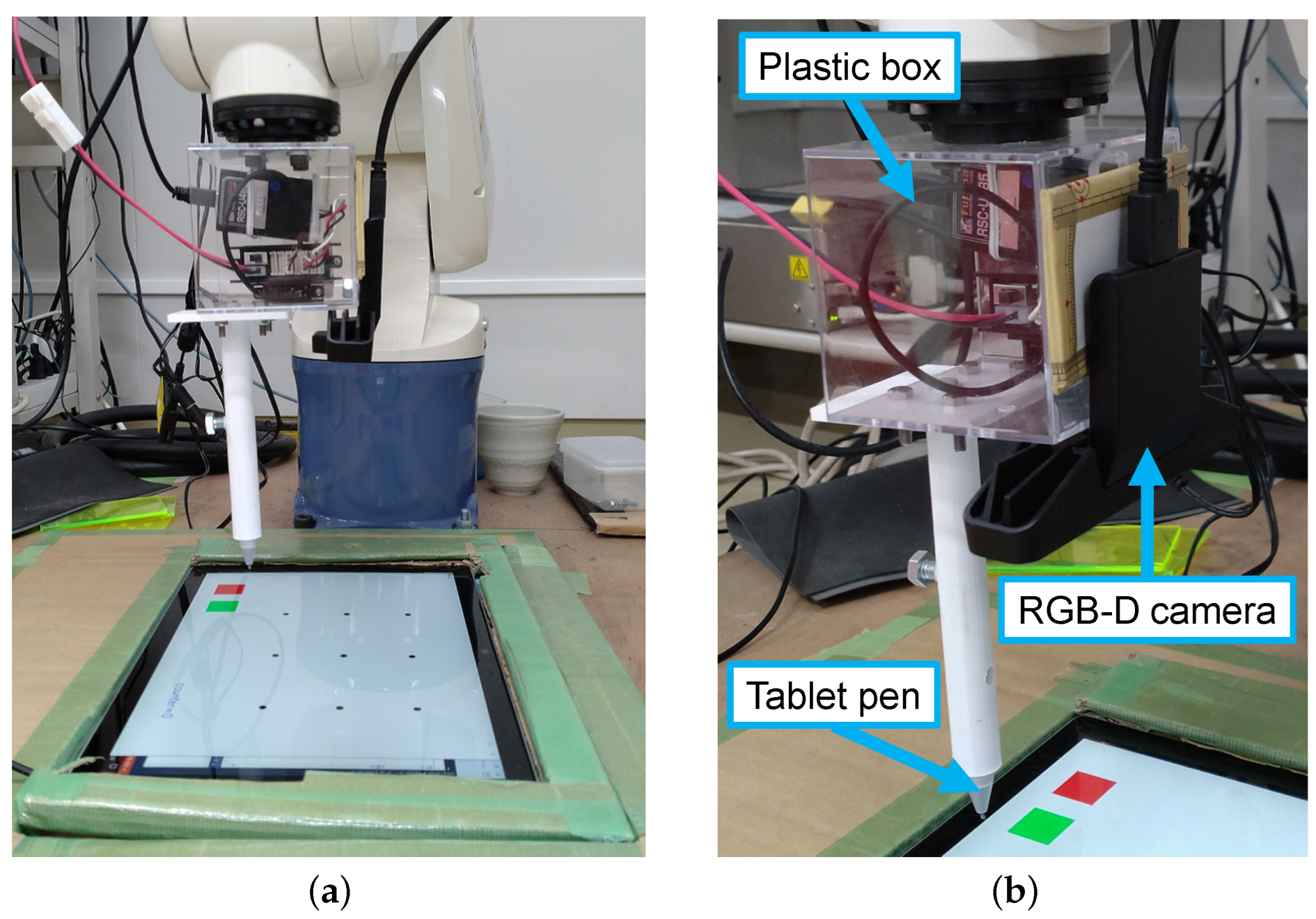
The developed system is shown in Figure 1. A clear plastic box is attached to the tip flange of the hand of a robot. An RGB-D camera and a tablet pen holder, which is fabricated by a 3D printer, are attached. Because an Intel SR300 camera is used, consideration of image distortion is not necessary [19]. In addition, the intrinsic parameters of the camera can be obtained easily by a software development kit (SDK). Both the pen and camera are mounted at positions different from the rotation center of the robot hand because the end-effector is handmade. Of course, there is no CAD model of it. The pen rotates when the hand rotates. It is necessary to calibrate in this scenario.

Figure 1.
(a) Appearance of the developed system; (b) details of the end-effector.
For hand–eye calibration using this developed system, some preparations are necessary, similar to the study of Hua [2]. Figure 2 shows a data processing procedure performed by the proposed method. First, nine landmarks (i.e., targets to touch by the robot’s hand with the tablet pen) are displayed on the tablet, as shown in Figure 1a. The interior area surrounded by landmarks is the considered workspace. Second, the tablet display is captured by the attached RGB-D camera, and all positions of the landmarks in the image coordinate system are obtained, as shown in Figure 3a. Third, the robot hand is manually operated to enable the pen and one landmark to touch each other, and the hand position in the robot-based coordinate system is acquired. This data acquisition is repeated to obtain all landmarks. Following this, the rotation angle of the sixth axis is gradually rotated; therefore, the first and ninth dots are and , respectively. Specifically, the sixth axis is rotated by . This is because the attached camera and pen are not aligned to the sixth axis of the robot hand, and calibrating in this scenario is necessary. Figure 3b shows an example of the acquired data. Because the attached pen is not aligned and the hand rotates, the data distribution in Figure 3b is different from that in Figure 3a. The parameters of the homogeneous transformation matrices (HTMs) are optimized by two-stage optimization. Using the optimized matrices, the positions to touch in the image coordinate system (Figure 3a) are converted to those in the robot-based coordinate system (Figure 3b). To evaluate the calibration performance, the robot hand with the attached pen touches the nine displayed landmarks, and the mean touching error is calculated after the optimized parameters are introduced in the robot.

Figure 2.
Data processing procedure.
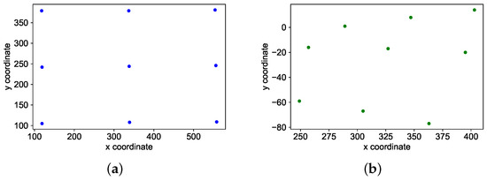
Figure 3.
(a) Positions of landmarks in the image coordinate system; (b) positions of the hand in the robot-based coordinate system.
3.2. Coordinate System and Homogeneous Transformation Matrix (HTM)
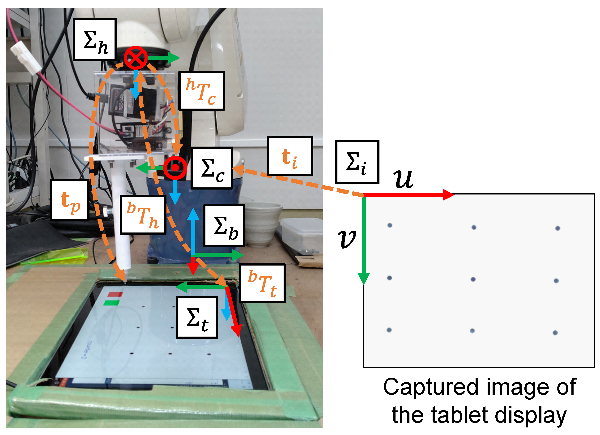
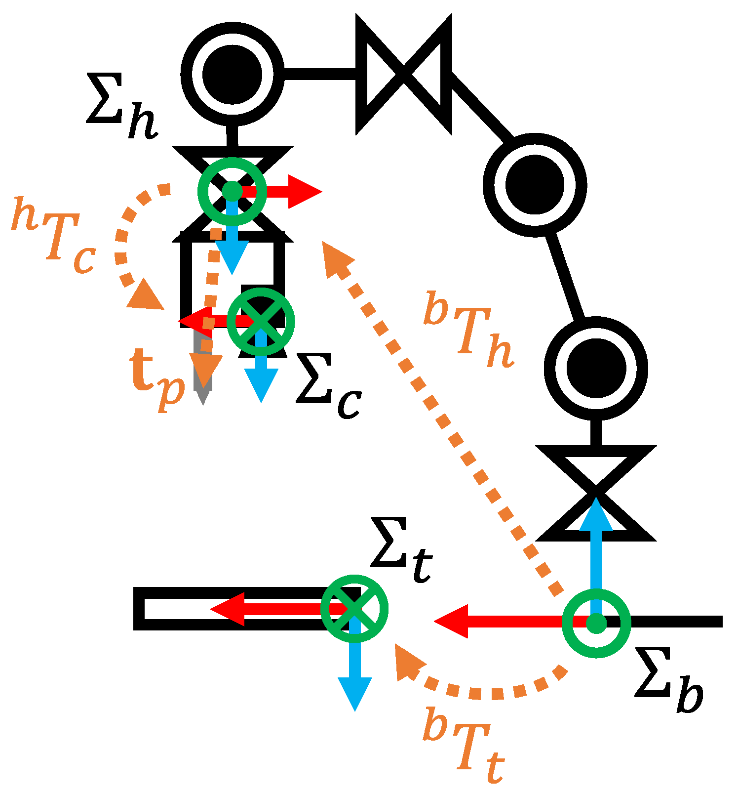
The used DENSO VP-6242 robot [20] has a range of motion with six degrees of freedom (DoF). The coordinate systems are shown in Figure 4 and Figure 5. , , , , and denote the robot base, hand, camera, image, and tablet computer coordinate systems. and represent HTMs, which have rotation and translation parts, as expressed below.
where and are translation vectors from to and to , respectively. , , and are rotation matrices of the x, y, and z axes, respectively.

Figure 4.
Coordinate systems. Red, green, and blue arrows represent x, y, and z axes, respectively. DENSO VP-6242 robot [20] is used.

Figure 5.
The free body diagram of the system.
represents the transformation from to . It can be achieved using the pinhole camera model.
where represents the mth black dot in . Let and be the focal lengths of the x and y axes, respectively. and are the coordinates of the principal points of the x and y axes, respectively. and are the transformed positions in . is the distance from the camera to the mth black dot. It is measured by the RGB-D camera. Thus,
Finally, the position in () can be obtained from the following equation:
In the developed system, the above equation is insufficient because the tablet pen and the camera are not aligned to the rotation axis of . Hence, the offset () should be considered, which can be calculated as follows:
As shown in Figure 4, is the translation vector from to the tip of the tablet pen. represents the rotation angle of the z-axis in . By combining Equations (5) and (7), the final equation is
3.3. Transformation from to
All positions of the black dots displayed on the tablet computer can be transformed from to . The position in px should be converted to mm as the first step using the following equation:
where , , PPI, and s are the converted result in mm, position in pixel, pixel per inch, and the display scale of the tablet computer, respectively. The PPI and s depend on a used tablet computer. The transformation from to is
where is the transformed result of the mth black dot, which is converted from px to mm () using Equation (9), in . is the translation vector from to . , , and are rotation angles of the x, y, and z axes of , respectively.
3.4. Representation by DH Method
The relationships of each coordinate system can be represented by the Denavit–Hartenberg (DH) method [21]. In contrast to the HTMs with the six-DoF mentioned above, four parameters , , , and are used in this method. Here, let and be the x and z axes of the nth link, respectively. These four parameters, respectively, denote the length of a common normal between the th and the nth links (link length), the angle of rotation around the from the to (link twist), the distance from the intersection of and to the origin of the ith link’s frame (link offset), and the angle of rotation around the from the to (joint angle). Using this method, Equation (5) can be rewritten.
The is an HTM in the DH method that represents the relationship between and . The can also be represented by the DH method; however, it can be acquired from the robot controller and it is considered a known quantity. The is a rotation matrix for each axis in the 3D space. Similarly, the relationship between the and can be rewritten as follows.
In addition to this approach, many other methods that represent the relationships of the coordinate system have been reported. In this study, a comparison of representations used by the 6-DoF HTM and DH methods was focused on.
3.5. Parameters to Be Optimized
The known and unknown parameters that should be optimized are listed (Table 1). In Equation (1), are known because they can be obtained from the robot controller. In Equation (2), can be approximately measured by hand. However, the manual measurement has an error and affects the final positioning error of the robot hand. Thus, they were optimized in this study. Because the robot hand is operated by causing the pen and the tablet display to touch each other, the optimization of is unnecessary. In the same equation, , , and are optimized. In Equation (3), , , , and are known because they can be obtained from the software development kit (SDK) of the RGB-D camera. is also known because the camera can measure the distance. In Equation (6), is known because a user sets the angle to rotate the hand. can be measured by hand; however, they should be optimized because of the above reasons. Similarly, can be ignored. In Equation (11), , , , , , and are unknown. However, can be ignored. Therefore, optimizing the 12 parameters is necessary for the six-DoF HTMs. For the DH method, the parameters of , , , and must be optimized. The and can be ignored for the same reason regarding , , and .

Table 1.
Known and unknown (should be optimized) parameters.
3.6. Two-Stage Optimization
To optimize the 12 unknown parameters and further minimize the positioning error of the robot hand, the developed method introduces a two-stage optimization. In the first stage, the 12 parameters are optimized based on the mathematical model described in Section 3.2. Using the optimized parameters, the positions of the black dots in (Figure 3a) can be converted to (Figure 3b). Thus, the robot hand with the tablet pen can touch the black dots of the tablet display. To further minimize the error, affine transformation-based optimization is introduced in the second stage.
3.6.1. First Optimization
Many optimization algorithms can be used. In this study, differential evolution (DE) [22] is adopted because of its ease of use. In DE, search points in a search space are referred to as individuals. Each individual includes a set of optimized parameters encoded as a vector. After the fitness of each individual is calculated using a fitness function, new individuals are generated for the next generation based on the calculated fitness, mutation, and crossover strategies. By iterating these procedures, the individuals gradually converge to an optimal solution.
In this study, the following equations are used for the fitness function.
where is the fitness function, and it consists of and . represents the mean Euclidean distance of the transformed nine black dots from to by Equation (5) and from to by Equation (10). This function is set because the transformed black dots by the different HTMs should match each other in if the unknown parameters in Equations (2) and (11) are optimized correctly.
To optimize the remaining unknown parameters in Equation (6), is introduced. If all unknown parameters are optimized correctly, and , which are calculated from Equation (8), as well as the hand positions in (Figure 3b), should match each other. However, when the data of the hand positions are the generated errors that occur, the generated data cannot be used as the perfect ground truth. The reason these errors occur is the difficulty in operating the robot hand manually to ensure that each center of the displayed landmarks and the tip of the tablet pen touch each other perfectly (with no distance error). To minimize the error as much as possible in the optimization process, Equation (20) is introduced. Let and be the created mth position of the robot hand in , where the pen and the mth black dot touch each other with a small distance error. and are the distance errors between the mth landmark and the touched position in . They can be obtained easily from the tablet computer in px. The unit can be converted to mm using Equation (9). This conversion is necessary before applying Equation (20).
3.6.2. Second Optimization
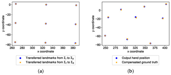
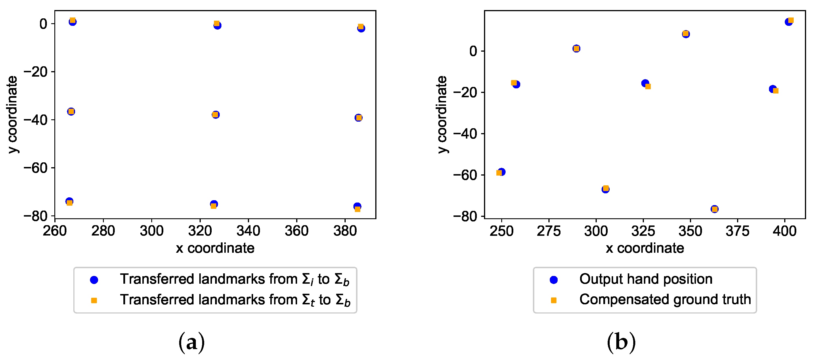
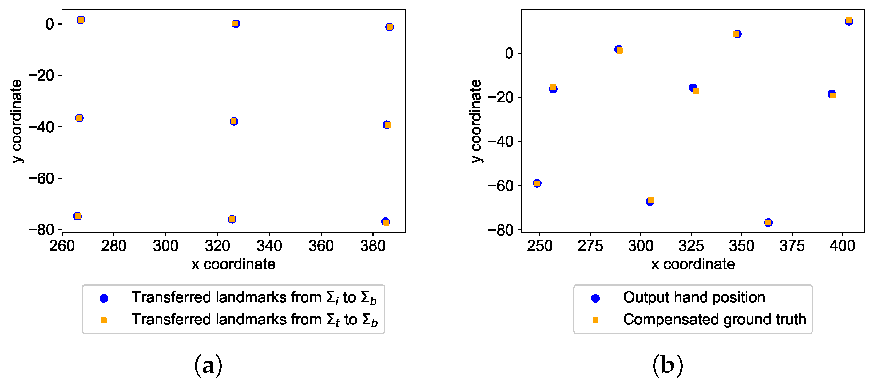
By the first optimization, a good calibration result of the six-DoF HTMs is confirmed, as shown in Figure 6. To further minimize the error, affine transformation matrices are optimized in the second stage to match the two data distributions more. For this purpose, the following fitness function is set:
where is the fitness function, which consists of and . They are almost the same as and . The difference is that affine transformation for a target position () is introduced. Let and be the amounts of translation of the x and y axes, respectively. and represent the centers of rotation of the x and y axes, respectively. In this study, the position of the fourth black dot was the center of rotation. is the angle of rotation. and are the scaling factors of the x and y axes, respectively.
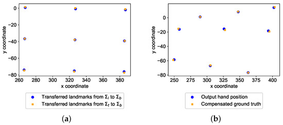
The unknown parameters to be optimized are , , , , and . Because ( and ), ten parameters should be optimized to match the two data distributions as much as possible. Figure 7 shows examples using the optimized affine transformation matrices and the six-DoF HTMs. The error decreases in both results. In the experiments, this effectiveness was evaluated quantitatively.
4. Experiment
4.1. Used Robot and Devices
In the experiments, a six-axis robot (DENSO VP-6242), a tablet computer (Microsoft Surface Pro 7), a tablet pen (Surface Pen), and an RGB-D camera (Intel SR300) were used. The positional repeatability of the robot was mm [20]. The resolution of the tablet was 267 ppi.
4.2. Data Creation
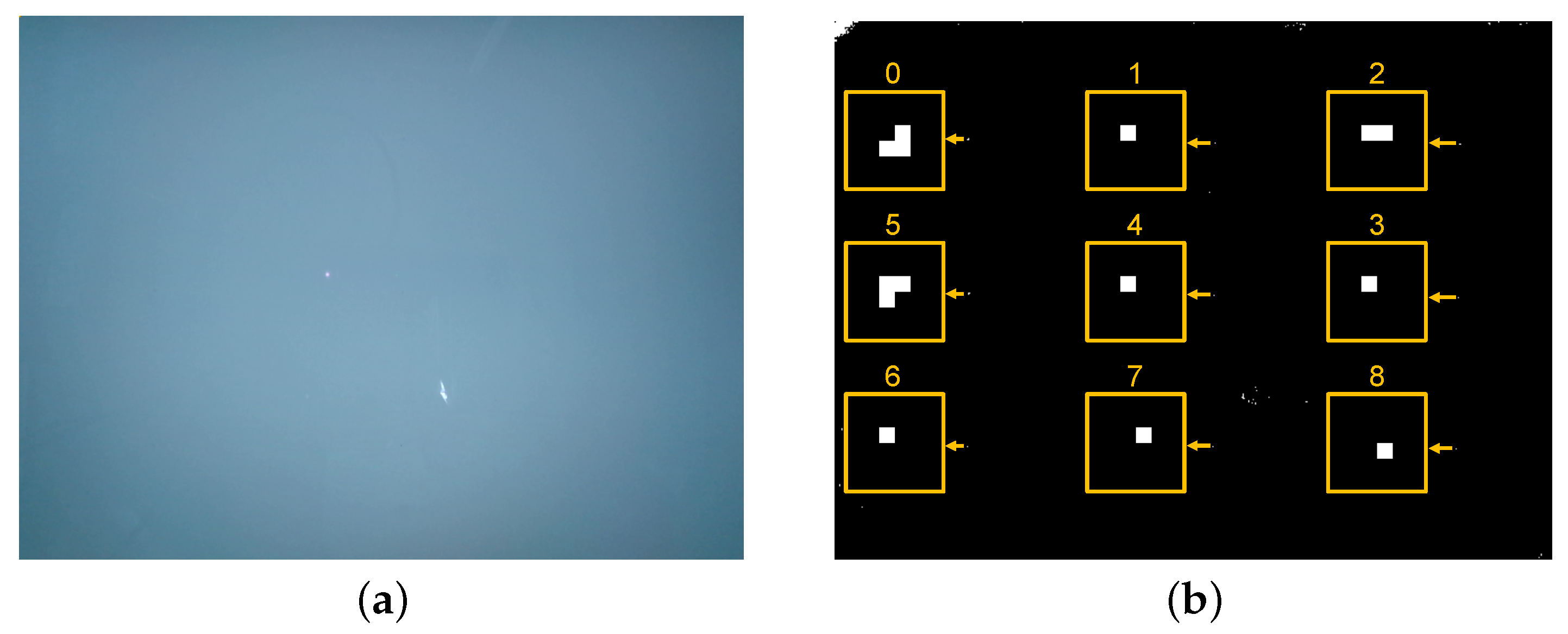
For the two-stage optimization, positions of the nine () displayed black dots in () and the corresponding positions of the robot hand in () are necessary. To create both data, first, nine black dots were displayed with one pixel (Figure 8a). Second, the tablet display was captured by the attached RGB-D camera. Third, the captured image was binarized, as shown in Figure 8b. Because one blob with a few pixels was obtained for each dot, the averaged coordinates are used as . Moreover, the corresponding depth data () of were acquired from the RGB-D camera.
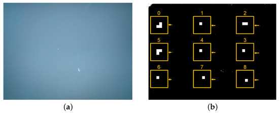
Figure 8.
(a) Captured image of the tablet display by RGB-D camera; (b) binarized image to detect displayed black dots.
Subsequently, the robot hand was operated such that the tip of the pen touched the displayed dots to create data as the ground truth. At this time, the touching error was obtained from the tablet computer to compensate for the error, as described in Section 3.6.1. Table 2 provides the created data.

Table 2.
Created data for two-stage optimization.
4.3. Set Values for Known Parameters
Table 3 presents the set values for the known parameters. represent the initial position of the robot hand to capture the tablet display. This position was determined by the author. , , , and were acquired from the SDK of the RGB-D camera [19]. is the rotation angle of the z-axis in to touch each displayed dot.

Table 3.
Set values for known parameters.
4.4. Setup for DE
Table 4 provides the set values for the hyperparameters of the DE. Let N and G be the population and the generation sizes, respectively. To avoid premature convergence, a sufficiently large size was set. As the crossover probability (CR) and the scaling factor (F), 0.9 and 0.5 were set, respectively. The binomial crossover and DE/rand/1 were adopted for the crossover and mutation strategies, respectively. Because the DE performance depended on a random seed, five different random seeds were used and compared in the two-stage optimization. Table 5 and Table 6 present the search ranges of the 12 optimized parameters for the 6-DoF HTMs and the DH method.

Table 4.
Set values for DE.

Table 5.
Search ranges of optimized parameters for six-DoF HTMs.

Table 6.
Search ranges for the DH method.
5. Results and Consideration
5.1. First-Stage Optimization
Table 7 summarizes the optimization results of the six-DoF HTMs using the five different random seeds. There are signed and unsigned values in and although all are the same. Hence, this optimization problem is multimodal. Because DE can exhibit good performance in a multimodal problem [22], using this algorithm is reasonable. All and were 0.64 and 1.04 mm, respectively. The absence of any error is attributed to the poor representation of the developed mathematical model or the inclusion of the measurement error in the depth information ().

Table 7.
Optimization results of the six-DoF HTMs after first-stage optimization.
Table 8 describes the optimization results of the DH method. Similar to the result of the six-DoF HTMs, all were the same. However, the values of some parameters were not identical. Thus, this optimization problem was also multimodal. The acquired values of were larger than the results of the six-DoF HTMs because the DH parameters were ill-conditioned. According to reference [21], adjacent joint axes of a real robot and end-effector are not perfectly parallel in practice owing to manufacturing tolerances and various types of errors. Therefore, the link length () can become extremely large. However, owing to the difficulty of precise prediction, the adjacent joint axes were assumed to be perfectly parallel in this experiment. This could cause values that are larger than those of the six-DoF HTMs.

Table 8.
Optimization results of the DH method after first-stage optimization.
Using the optimized values of seed 1 of the 6-DoF HTMs, the mean touching error was measured by making the robot hand touch all displayed dots. Table 9 presents the result. Equation (9) with and was used to convert the px to mm because Microsoft Surface Pro 7 was used. A mean touching error of 1.25 mm was achieved.

Table 9.
Demonstration result after first-stage optimization.
5.2. Second-Stage Optimization
Using the optimized parameters of seed 1 in the first-stage optimization, parameters for the two affine transformation matrices are optimized in the second-stage optimization. Table 10 summarizes the results for the six-DoF HTMs. Because the decreased compared to , the second optimization contributes to reducing the error. Although different random seeds are set, all results are identical. Hence, the possibility of premature convergence is low, showing that these optimization results are reliable.

Table 10.
Optimization results in second-stage optimization for the six-DoF HTMs.
Table 11 presents the results of the DH method. Similar to the six-DoF HTMs, all values are the same. Because the result of the first-stage optimization is worse, the result of the second-stage optimization was also worse.

Table 11.
Optimization results after second-stage optimization for the DH method.
DH method represents a relationship of reference frames using four parameters, whereas HTM, which is often used in hand–eye calibration, uses six. Thus, the lower computational cost of the DH method is among its notable advantages. However, it does involve a few disadvantages as mentioned in the reference [21]. As described above, DH parameters have ill-conditioned behavior because the link length becomes extremely large when adjacent joint axes are not perfectly parallel. Moreover, link frames must be assigned such that valid DH parameters exist and arbitrary assignment is impossible. In contrast, six-DoF HTMs can be assigned. Thus, they are easy to use. As shown in the results of the two-stage optimizations, six-DoF HTMs achieve better results. Thus, this representation is suitable for hand–eye calibration.
Using all optimized parameters for the six-DoF HTMs, the mean touching error is measured. Hand positions to touch are calculated using the below equations.
Because the robot hand always touches the tablet display, the calculation of is unnecessary. Table 12 presents the results. Compared to the previous result, the mean touching error decreases. Thus, the affine transformation-based error minimization is effective. Because the mean touching errors in all trial numbers decrease, this method is stable.

Table 12.
Demonstration results after second-stage optimization.
6. Conclusions
In this study, a method that has the advantages of a traditional hand–eye calibration approach and a neural network-based approach is proposed. Simple mathematical models of six-DoF HTMs and the DH method were developed and optimized using the data, which were created using the attached end-effector. Therefore, the proposed method can provide numerical and quantitative results to users and researchers. Additional calibration for the end-effector can be avoided, although there is no CAD model because the data are created using the attached end-effector. Two-stage optimization was introduced to optimize the mathematical models. In the first-stage optimization, 12 parameters of the transformation matrices, which converted a position in the image coordinate system to that in the robot-based coordinate system to touch, were optimized. To further minimize the error, ten parameters of the two affine transformation matrices were optimized in the second-stage optimization. Using these optimized parameters, a mean touching error of 1.0 mm was achieved by the six-DoF HTMs. Because the proposed method can optimize the mathematical model using the data generated by the attached end-effector without detailed information, such as CAD diagrams, this method incorporates the advantages of both approaches, in contrast to conventional systems.
For smaller errors, developing a new method will be a future research direction. Additionally, similar to existing calibration methods, the proposed method requires recalibration if a different end-effector with different dimensions is attached. As this is a tedious process, a method that utilizes the first calibration result must be developed in future research to reduce the efforts required to perform the recalibration procedure.
Funding
This research received no external funding.
Conflicts of Interest
The authors declare no conflict of interest.
References
- Lin, W.; Liang, P.; Luo, G.; Zhao, Z.; Zhang, C. Research of Online Hand-Eye Calibration Method Based on ChArUco Board. Sensors 2022, 119, 3805. [Google Scholar]
- Hua, J.; Zeng, L. Hand-Eye Calibration Algorithm Based on an Optimized Neural Network. Actuators 2021, 10, 85. [Google Scholar] [CrossRef]
- Enebuse, I.; Foo, M.; Ibrahim, B.S.K.K.; Ahmed, H.; Supmak, F.; Eyobu, O.S. A Comparative Review of Hand-Eye Calibration Techniques for Vision Guided Robots. IEEE Access 2021, 9, 113143–113155. [Google Scholar] [CrossRef]
- Jiang, J.; Luo, X.; Luo, Q.; Qiao, L.; Li, M. An Overview of Hand-Eye Calibration. Int. J. Adv. Manuf. Technol. 2022, 22, 77–97. [Google Scholar]
- Shiu, Y.C.; Ahmad, S. Calibration of wrist-mounted robotic sensors by solving homogeneous transform equations of the form AX = XB. IEEE Trans. Robot. Autom. 1989, 5, 16–29. [Google Scholar]
- Motai, Y.; Kosaka, A. Hand-Eye Calibration Applied to Viewpoint Selection for Robotic Vision. IEEE Trans. Ind. Electron. 2008, 55, 3731–3741. [Google Scholar]
- Tsai, R.Y.; Lenz, R.K. A new technique for fully autonomous and efficient 3D robotics hand/eye calibration. IEEE Trans. Robot. Autom. 1989, 5, 345–358. [Google Scholar]
- Wang, C.C. Extrinsic calibration of a vision sensor mounted on a robot. IEEE Trans. Robot. Autom. 1992, 8, 161–175. [Google Scholar]
- Park, F.C.; Martin, B.J. Robot sensor calibration: Solving AX = XB on the Euclidean group. IEEE Trans. Robot. Autom. 1994, 10, 717–721. [Google Scholar] [CrossRef]
- Ma, S.D. A self-calibration technique for active vision systems. IEEE Trans. Robot. Autom. 1996, 12, 114–120. [Google Scholar]
- Daniilidis, K. Hand-Eye Calibration Using Dual Quaternions. Int. J. Robot. Res. 1999, 18, 286–298. [Google Scholar]
- Horaud, R.; Dornaika, F. Hand-Eye Calibration. Int. J. Robot. Res. 1995, 14, 195–210. [Google Scholar] [CrossRef]
- Andreff, N.; Horaud, R.; Espiau, B. Robot Hand-Eye Calibration using Structure from Motion. Int. J. Robot. Res. 2001, 20, 228–248. [Google Scholar]
- Zhao, Z. Hand-eye calibration using convex optimization. In Proceedings of the IEEE International Conference on Robotics and Automation, Shanghai, China, 9–13 May 2011; pp. 2947–2952. [Google Scholar]
- Heller, J.; Havlena, M.; Pajdla, T. Globally Optimal Hand-Eye Calibration Using Branch-and-Bound. IEEE Trans. Pattern Anal. Mach. Intell. 2016, 38, 1027–1033. [Google Scholar] [PubMed]
- Zhuang, H.; Roth, Z.; Sudhakar, R. Simultaneous robot/world and tool/flange calibration by solving homogeneous transformation equations of the form AX = YB. IEEE Trans. Robot. Autom. 1994, 10, 549–554. [Google Scholar] [CrossRef]
- Mišeikis, J.; Glatte, K.; Elle, O.J.; Torresen, J. Automatic Calibration of a Robot Manipulator and Multi 3D Camera System. In Proceedings of the IEEE/SICE International Symposium on System Integration, Sapporo, Japan, 13–15 December 2016; pp. 735–741. [Google Scholar]
- Koide, K.; Menegatti, E. General Hand-Eye Calibration Based on Reprojection Error Minimization. IEEE Robot. Autom. Lett. 2019, 4, 1021–1028. [Google Scholar] [CrossRef]
- Projection in Intel RealSense SDK 2.0. Available online: https://dev.intelrealsense.com/docs/projection-in-intel-realsense-sdk-20 (accessed on 19 January 2023).
- DENSO ROBOT USER MANUALS. Available online: http://eidtech.dyndns-at-work.com/support/RC8_Manual/005929.html (accessed on 19 January 2023).
- Lynch, K.M.; Park, F.C. Modern Robotics: Mechanics, Planning, and Control; Cambridge University Press: Cambridge, UK, 2017. [Google Scholar]
- Das, S.; Suganthan, P.N. Differential Evolution: A Survey of the State-of-the-Art. IEEE Trans. Evol. Comput. 2011, 15, 4–31. [Google Scholar]
Disclaimer/Publisher’s Note: The statements, opinions and data contained in all publications are solely those of the individual author(s) and contributor(s) and not of MDPI and/or the editor(s). MDPI and/or the editor(s) disclaim responsibility for any injury to people or property resulting from any ideas, methods, instructions or products referred to in the content. |
© 2023 by the author. Licensee MDPI, Basel, Switzerland. This article is an open access article distributed under the terms and conditions of the Creative Commons Attribution (CC BY) license (https://creativecommons.org/licenses/by/4.0/).

