Comparison of Two Aspects of a PDE Model for Biological Network Formation

Abstract

We compare the solutions of two systems of partial differential equations (PDEs), seen as two different interpretations of the same model which describes the formation of complex biological networks. Both approaches take into account the time evolution of the medium flowing through the network, and we compute the solution of an elliptic–parabolic PDE system for the conductivity vector m, the conductivity tensor $\mathbb{C}$ and the pressure p. We use finite differences schemes in a uniform Cartesian grid in a spatially two-dimensional setting to solve the two systems, where the parabolic equation is solved using a semi-implicit scheme in time. Since the conductivity vector and tensor also appear in the Poisson equation for the pressure p, the elliptic equation depends implicitly on time. For this reason, we compute the solution of three linear systems in the case of the conductivity vector $m\in {\mathbb{R}}^2$ and four linear systems in the case of the symmetric conductivity tensor $\mathbb{C}\in {\mathbb{R}}^{2\times 2}$ at each time step. To accelerate the simulations, we make use of the Alternating Direction Implicit (ADI) method. The role of the parameters is important for obtaining detailed solutions. We provide numerous tests with various values of the parameters involved to determine the differences in the solutions of the two systems.

1. Introduction

We study two elliptic–parabolic systems of partial differential equations (PDEs) describing the formation of biological network structures. Both systems are derived as gradient flows of an energy functional, consisting of a diffusive term, activation term and metabolic cost term. The energy functional can be seen as a continuum version of its discrete counterpart introduced in [1]. Here, the authors consider a total energy consumption function for a general class of biological transport networks (seen also in [2]), including a material cost function of the network. In the papers [1,3], the authors adapt the dynamics of local information for a biological transport network and its relation with the optimization principle, which is known to be very common in nature.

Assuming the validity of Darcy’s law for slow flow in porous media (see, for instance, [4,5]), the energy functional is constrained by a Poisson equation for the fluid pressure. We use two modes of description of the network conductivity: first, in terms of a conductance vector m, and, second, in terms of a symmetric positive definite conductance tensor $\mathbb{C}$. Taking the $L^2$-gradient flow with respect to m (see, for instance, [6,7,8,9,10]) and, resp., with respect to $\mathbb{C}$ (see [11]), leads to two structurally similar elliptic–parabolic PDE systems.

In the parabolic equation, a reaction term appears, representing the metabolic cost of the network, while the diffusion term describes the randomness in the material structure. The third term, called the activation term, describes the tendency of the network to align with the principal direction of the material flow. The elliptic Poisson equation describes local mass conservation and is equipped with a right-hand side describing the distribution of sources and sinks of the material. This distribution is supplied as a datum and is supposed to be time-independent.

The aim of this paper is to present several numerical simulations of both the vector-valued m model and the tensor-valued $\mathbb{C}$ model, with the goal of comparing their solutions in various parameter settings. The initial datum is chosen such that $\mathbb{C}=m\otimes m$, i.e., initially, the principal direction (the eigenvector corresponding to the largest eigenvalue) of $\mathbb{C}$ is aligned with m. Note that, in the spatially two-dimensional setting, the second eigenvalue of $m\otimes m$ is zero, with eigenspace orthogonal to m. We shall observe that the two PDE systems develop structurally and qualitatively similar solutions; however, they differ in quantitative details, for instance, the number and location of branches.

2. Mathematical Model

We introduce the energy functional ${\mathcal{E}}_{\mathrm{tens}}$ for the tensor-valued model,

$${\mathcal{E}}_{\mathrm{tens}}\left[\mathbb{C}\right]:={\int }_{\mathsf{\Omega }}\frac{D^2}{2}{|\nabla \mathbb{C}|}^2+c^2\nabla p\left[\mathbb{C}\right]·\mathbb{P}\left[\mathbb{C}\right]\nabla p\left[\mathbb{C}\right]+M\left(\right|\mathbb{C}\left|\right)\mathrm{d}x,$$

(1)

where $\mathbb{C}=\mathbb{C}\left(x\right)\in {\mathbb{R}}^{2\times 2}$ is the conductivity tensor, the diffusivity parameter $D\in \mathbb{R}$ measures the effect of random fluctuations in the network, and the activation parameter $c^2>0$ controls the strength of the network formation feedback loop. The total permeability tensor is of the form $\mathbb{P}\left[\mathbb{C}\right]:=r\mathbb{I}+\mathbb{C}$, where the scalar function $r=r\left(x\right)\ge r_0>0$ describes the isotropic background permeability of the medium. The scalar pressure $p=p\left[\mathbb{C}\right]$ of the fluid transported within the network is the unique solution (up to an additive constant) of the Poisson equation

$$-\nabla ·\left(\mathbb{P}\left[\mathbb{C}\right]\nabla p\right)=S,$$

(2)

subject to homogeneous Neumann boundary condition on $\partial \Omega$. The source/sink distribution $S=S\left(x\right)$ in the mass conservation Equation (2) is to be supplemented as an input datum and is assumed to be independent of time. The metabolic cost function $M:{\mathbb{R}}^{+}\to {\mathbb{R}}^{+}$ describes the dependence of the metabolic expenditure of maintaining the network on its transportation capacity; see [1]. The expression $\left|\mathbb{C}\right|$ denotes the Frobenius norm $\left|\mathbb{C}\right|:=\sqrt{{\sum }_{i=1}^2{\sum }_{j=1}^2{C}_{ij}^2}$ and $|\nabla \mathbb{C}|:=\sqrt{{\sum }_{i=1}^2{\sum }_{j=1}^2{\sum }_{k=1}^2{(\partial C_{ij}/\partial x_k)}^2}$.

Taking the $L^2$-gradient flow of the energy (1) constrained by (2), we obtain the parabolic–elliptic system

$$\begin{array}{cc}\hfill -\nabla ·\left(\left(r\mathbb{I}+\mathbb{C}\right)\nabla p\right)& =S\hfill \end{array}$$

(3)

$$\begin{array}{cc}\hfill \frac{\partial \mathbb{C}}{\partial t}-D^2\Delta \mathbb{C}-c^2\nabla p\otimes \nabla p+\frac{M^{\prime }\left(\left|\mathbb{C}\right|\right)}{\left|\mathbb{C}\right|}\mathbb{C}& =0;\hfill \end{array}$$

(4)

see [11] for details of the derivation. In our paper, we shall make the generic choice for the metabolic cost function (see, e.g., [6,7,8,9]),

$$M\left(s\right):=\frac{\alpha }{\gamma }{s}^{\gamma }\mathrm{for} s\ge 0,$$

(5)

where $\alpha >0$ is the metabolic constant and $\gamma >0$ the metabolic exponent. For instance, to model leaf venation in plants, one chooses $1/2<\gamma <1$; see [1]. Then, Equation (4) becomes

$$\frac{\partial \mathbb{C}}{\partial t}-D^2\Delta \mathbb{C}-c^2\nabla p\otimes \nabla p+\alpha {\left|\mathbb{C}\right|}^{\gamma -2}\mathbb{C}=0$$

(6)

To derive the vector-valued model, we make the ansatz $\mathbb{C}:=m\otimes m$. Inserting this into (1) with $D=0$ and noting that $\left|\mathbb{C}\right|={\left|m\right|}^2$, we obtain

$$\mathcal{E}={\int }_{\Omega }{c}^2\nabla p\left[m\right]·\mathbb{P}\left[m\right]\nabla p\left[m\right]+M\left({\left|m\right|}^2\right)\mathrm{d}x$$

with $\mathbb{P}\left[m\right]=r\mathbb{I}+m\otimes m$ and, with a slight abuse of notation, we now denote by $p=p\left[m\right]$ the solution of the Poisson Equation (2) with $\mathbb{P}\left[\mathbb{C}\right]$ replaced by $\mathbb{P}[m\otimes m]$. Re-introducing the Dirichlet integral $D^2{\int }_{\Omega }{|\nabla m|}^2\mathrm{d}x$, we arrive at the energy functional

$${\mathcal{E}}_{\mathrm{vect}}\left[m\right]:={\int }_{\Omega }{D}^2{|\nabla m|}^2+c^2\nabla p\left[m\right]·\mathbb{P}[m\otimes m]\nabla p\left[m\right]+{M\left(\right|m|}^2)\mathrm{d}x.$$

(7)

Note that this functional is different from the one obtained by replacing $\mathbb{C}=m\otimes m$ in Equation (1), with the two functionals mainly differencing in the contribution of the diffusion term. As we shall see, we are mainly interested in studying the behavior of the system for very small diffusion coefficients, so that we expect such difference to not be so crucial.

Taking the $L^2$-gradient flow with respect to the vector variable m and using the explicit form (5) for the metabolic function, we obtain the system

$$\begin{array}{cc}\hfill -\nabla ·\left(\left(r\mathbb{I}+m\otimes m\right)\nabla p\right)& =S\hfill \end{array}$$

(8)

$$\begin{array}{cc}\hfill \frac{\partial m}{\partial t}-D^2\Delta m-c^2(\nabla p\otimes \nabla p)m+\alpha {\left|m\right|}^{2(\gamma -1)}m& =0.\hfill \end{array}$$

(9)

From now on, we denote system (3) and (6) as the $\mathbb{C}$ system (or model), while we call (8) and (9) the m system (or model). Let us now shortly discuss the differences between the two systems. First, the activation term $c^2\nabla p\otimes \nabla p$ in (4) is quadratic and depends on $\mathbb{C}$ only through the solution $p=p\left[\mathbb{C}\right]$ of the Poisson Equation (3). In contrast, the activation term $c^2(\nabla p\otimes \nabla p)m$ in (9) is cubic. Moreover, the metabolic term ${\alpha \left|\mathbb{C}\right|}^{\gamma -2}\mathbb{C}$ in (4), which comes from the gradient flow, where the gradient of the functional defined in Equation (1) is taken with respect to $\mathbb{C}$, becomes singular at $\mathbb{C}=0$ if (and only if) $\gamma <1$. This obviously causes difficulties for both the analytical treatment of the system (see [11] for details) and its numerical resolution. We discuss in Section 3.2.1 how the numerical difficulties can be overcome. In contrast, the metabolic term ${\alpha \left|m\right|}^{2(\gamma -1)}m$ in (9) only becomes singular at $m=0$ if $\gamma <1/2$. Taking into account the fact that for typical applications in biology, only the parameter range $\gamma \ge 1/2$ is relevant (see [1]), the metabolic term in (9) does not require any special treatment for the m system. We point out that the different expressions for the metabolic terms, in the $\mathbb{C}$ and the m models, come from the fact that in defining the gradient flows, we differentiate the energy functionals defined in Equations (1) and (7) with respect to $\mathbb{C}$ and m, respectively.

We define the equations on a domain $\Omega \subset {\mathbb{R}}^2$, and we define the boundary conditions on $\partial \Omega$ for the pressure and the conductivity. We choose homogeneous Dirichlet boundary conditions for m and $\mathbb{C}$ and homogeneous Neumann conditions for p.

$$m(t,\overrightarrow{x})=0,\mathbb{C}(t,\overrightarrow{x})=0,\mathbb{P}\left[\mathbb{C}\right]\nabla p(t,\overrightarrow{x})·\nu =0,\overrightarrow{x}\in \partial \Omega ,t\ge 0$$

(10)

where $\nu$ is the outgoing normal vector to $\partial \Omega$. In all our numerical tests, the numerical support of $\mathbb{C}$ or m, after a long time, is well within $\Omega$; therefore, the solution should not be particularly sensitive to the boundary conditions on the two variables. In any case, different boundary conditions for m and $\mathbb{C}$ are currently under investigation.

To close the system, we prescribe an initial condition for the conductivity vector and tensor

$$m(t=0,\overrightarrow{x})=m^0\left(\overrightarrow{x}\right),\mathbb{C}(t=0,\overrightarrow{x})={\mathbb{C}}^0\left(\overrightarrow{x}\right),\mathrm{in}\Omega .$$

(11)

A direct consequence of the boundary condition defined for the pressure, which is also a necessary condition for the solvability of the Poisson equation, is that the source function has to be the vanishing mean, i.e., ${\displaystyle {\int }_{\Omega }S\left(\overrightarrow{x}\right)d\Omega =0}$.

3. Numerical Schemes

In this section, we define the numerical schemes used to discretize Equations (3), (4), (8) and (9) in space and time. We adopt semi-implicit second-order schemes.

3.1. Space Discretization

In space, we consider the square domain $\Omega =[0,1]\times [0,1]$, which we discretize by a uniform Cartesian mesh with spatial step $h:=\Delta x=\Delta y$. We call ${\Omega }_h$ the discrete computational domain. The two variables of conductivity and the pressure are ${\mathbb{C}}_{ij}\approx \mathbb{C}(x_i,y_j),m_{ij}\approx m(x_i,y_j)$ and $p_{ij}\approx p(x_i,y_j)$, defined at the center of the cell $(i,j)$; therefore, the set of grid points is $x_i=(i-1/2)h,y_j=(j-1/2)h,(i,j)\in {\{1,\cdots ,N\}}^2$, $hN=1$.

In order to obtain second-order accuracy in space, we use central differences for the computation of the space derivatives [12]. Discretizing Equation (9) in space, we have:

$$\begin{array}{ccc}\hfill {\displaystyle \frac{\partial m^{\left(1\right)}}{\partial t}}& =& D^2\mathcal{L}{m}^{\left(1\right)}+c^2{\left({\mathcal{D}}_{x}p\right)}^2{m}^{\left(1\right)}+c^2{\mathcal{D}}_{x}p{\mathcal{D}}_{y}p{m}^{\left(2\right)}-\alpha {\left|m\right|}^{2(\gamma -1)}{m}^{\left(1\right)}\hfill \end{array}$$

(12)

$$\begin{array}{ccc}\hfill {\displaystyle \frac{\partial m^{\left(2\right)}}{\partial t}}& =& D^2\mathcal{L}{m}^{\left(2\right)}+c^2{\left({\mathcal{D}}_{y}p\right)}^2{m}^{\left(2\right)}+c^2{\mathcal{D}}_{x}p{\mathcal{D}}_{y}p{m}^{\left(1\right)}-\alpha {\left|m\right|}^{2(\gamma -1)}{m}^{\left(2\right)}\hfill \end{array}$$

(13)

while the semi-discrete version of Equation (4) is

$$\begin{array}{ccc}\hfill {\displaystyle \frac{\partial C^{(1,1)}}{\partial t}}& =& D^2\mathcal{L}{C}^{(1,1)}+c^2{\left({\mathcal{D}}_{x}p\right)}^2-\alpha {\left|\mathbb{C}\right|}^{\gamma -2}{C}^{(1,1)}\hfill \end{array}$$

(14)

$$\begin{array}{ccc}\hfill {\displaystyle \frac{\partial C^{(1,2)}}{\partial t}}& =& D^2\mathcal{L}{C}^{(1,2)}+c^2{\mathcal{D}}_{x}p{\mathcal{D}}_{y}p-\alpha {\left|\mathbb{C}\right|}^{\gamma -2}{C}^{(1,2)}\hfill \end{array}$$

(15)

$$\begin{array}{ccc}\hfill {\displaystyle \frac{\partial C^{(2,2)}}{\partial t}}& =& D^2\mathcal{L}{C}^{(2,2)}+c^2{\left({\mathcal{D}}_{y}p\right)}^2-\alpha {\left|\mathbb{C}\right|}^{\gamma -2}{C}^{(2,2)}\hfill \end{array}$$

(16)

where $\mathcal{L}$ is the discrete Laplacian operator and ${\mathcal{D}}_x$ and ${\mathcal{D}}_y$ are, respectively, the discrete x and y first derivative operators, both using central difference approximation. The norm $|·|$ we use is the Frobenius one. In this case, we have three equations instead of four, because $\mathbb{C}$ is symmetric.

In order to have a fully implicit scheme, we define a compact form of the semi-discrete Equations (12) and (13) and Equations (14) and (16), as follows:

$$\begin{array}{ccc}\hfill {\displaystyle \frac{\partial m_{\mathrm{comp}}}{\partial t}}& =& D^2\mathcal{L}{m}_{\mathrm{comp}}+c^2\mathcal{P}{m}_{\mathrm{comp}}-\alpha {\mathcal{Q}}^m\left(m\right)m_{\mathrm{comp}}\hfill \end{array}$$

(17)

$$\begin{array}{ccc}\hfill {\displaystyle \frac{\partial {\mathbb{C}}_{\mathrm{comp}}}{\partial t}}& =& D^2\mathcal{L}{\mathbb{C}}_{\mathrm{comp}}+c^2\mathcal{P}-\alpha {\mathcal{Q}}^c\left(\mathbb{C}\right){\mathbb{C}}_{\mathrm{comp}}\hfill \end{array}$$

(18)

where $m_{\mathrm{comp}}={[m^{\left(1\right)},m^{\left(2\right)}]}^T$, ${\mathbb{C}}_{\mathrm{comp}}={[C^{(1,1)},C^{(1,2)},C^{(2,2)}]}^T$ and $\mathcal{P}={\mathcal{D}}_{\beta }p{\mathcal{D}}_{\eta }p$, with the suitable choice of $\beta ,\eta \in \{x,y\}$. For the metabolic terms, we have

$$\begin{array}{ccc}\hfill {\mathcal{Q}}^m\left(m\right)& =& {\left|m\right|}^{2(\gamma -1)}\hfill \end{array}$$

(19)

$$\begin{array}{ccc}\hfill {\mathcal{Q}}^c\left(\mathbb{C}\right)& =& {\left|\mathbb{C}\right|}^{\gamma -2}.\hfill \end{array}$$

(20)

Here, we discretize the Poisson equation for the pressure. To obtain a conservative scheme, we consider the following discretization: first, we extend the formula in Equation (3), which becomes

$$\begin{array}{c}\hfill {\partial }_x\left(\left(r+C^{(1,1)}\right){\partial }_{x}p\right)+{\partial }_x\left(C^{(1,2)}{\partial }_{y}p\right)+{\partial }_y\left(C^{(1,2)}{\partial }_{x}p\right)+{\partial }_y\left(\left(r+C^{(2,2)}\right){\partial }_{y}p\right)=-S\end{array}$$

(21)

where we use the symmetry $C^{(1,2)}=C^{(2,1)}$.

Now, we discretize the components of the formula, one by one, since we use different discretizations. For simplicity, we pose ${\mathcal{C}}^{1,1}=r+C^{(1,1)}$:

$$\begin{array}{cc}\hfill {\partial }_x{\left({\mathcal{C}}^{1,1}{\partial }_{x}p\right)}_{i,j}\approx & \frac{1}{\Delta x}\left({\mathcal{C}}_{i+1/2,j}^{1,1}{\partial }_x{p}_{i+1/2,j}-{\mathcal{C}}_{i-1/2,j}^{1,1}{\partial }_x{p}_{i-1/2,j}\right)\hfill \\ \hfill =& \frac{1}{2\Delta x^2}\left(\left({\mathcal{C}}_{i+1,j}^{1,1}+{\mathcal{C}}_{i,j}^{1,1}\right)p_{i+1,j}+\left({\mathcal{C}}_{i-1,j}^{1,1}+{\mathcal{C}}_{i,j}^{1,1}\right)p_{i-1,j}\right)\hfill \\ \hfill & -\frac{1}{2\Delta x^2}\left({\mathcal{C}}_{i+1,j}^{1,1}+{\mathcal{C}}_{i-1,j}^{1,1}+2{\mathcal{C}}_{i,j}^{1,1}\right)p_{i,j}\hfill \end{array}$$

(22)

where, in the last line, we consider the following approximations:

$${\partial }_x{p}_{i+1/2,j}\approx \frac{p_{i+1,j}-p_{i,j}}{\Delta x},{\mathcal{C}}_{i+1/2,j}^{1,1}\approx \frac{{\mathcal{C}}_{i+1,j}^{1,1}+{\mathcal{C}}_{i,j}^{1,1}}{2}.$$

We omit the term with both y derivatives because it is analog to the one with x derivatives. Now, we discretize the term with mix derivatives.

$$\begin{array}{cc}\hfill {\partial }_x{\left(C^{(1,2)}{\partial }_{y}p\right)}_{i,j}\approx & \frac{1}{\Delta x}\left(C_{i+1/2,j}^{(1,2)}{\partial }_y{p}_{i+1/2,j}-C_{i-1/2,j}^{(1,2)}{\partial }_y{p}_{i-1/2,j}\right)\hfill \\ \hfill =& \frac{1}{8\Delta x^2}\left(C_{i+1,j}^{(1,2)}+C_{i,j}^{(1,2)}\right)(p_{i+1,j+1}-p_{i+1,j-1})\hfill \end{array}$$

(23)

$$\begin{array}{cc}& -\frac{1}{8\Delta x^2}\left(C_{i-1,j}^{(1,2)}+C_{i,j}^{(1,2)}\right)(p_{i-1,j+1}-p_{i-1,j-1})\hfill \end{array}$$

(24)

$$\begin{array}{cc}\hfill & +\frac{1}{8\Delta x^2}\left(C_{i+1,j}^{(1,2)}-C_{i-1,j}^{(1,2)}\right)(p_{i,j+1}-p_{i,j-1})\hfill \end{array}$$

(25)

Again, we omit the term with $y,x$ derivatives because it is analog to the one with $x,y$ derivatives.

3.2. Time Discretization: Symmetric ADI Method

At this stage, we describe the time discretization that we apply to the model. Since systems (3), (4), (6) and (8) are stiff in all their components, the choice of the time discretization is crucial for the efficiency.

We also need a high-performing scheme in time, since at each time step, we compute the solution of seven linear systems (two for the conductivity vector m, three for the conductivity tensor $\mathbb{C}$ and two Poisson equations for the pressure p).

As we shall see, for some values of the parameters, the well-posedness of the problem becomes weaker, which reflects the bad conditioning of the numerical problem. For such a reason, we adopt a symmetric scheme, which better preserves possible symmetries of the solution. In particular, we adopt a symmetric ADI scheme for both the conductivity variables, which guarantees efficiency, second-order accuracy and spatial symmetry.

Anyway, the scheme is not strictly second-order accurate in time for two reasons. First, the pressure is computed at time n rather than at an intermediate time $n+1/2$. Second, the metabolic term is treated partially explicitly and partially implicitly, thus destroying second-order accuracy. Improvements in the order of accuracy in time are currently under investigation.

3.2.1. Time Discretization for the Conductivity Vector

Here, we focus on the time discretization for Equations (8) and (9).

Given $m^n\approx m\left(t^n\right)$, we compute $p^n$ by solving the Poisson equation

$$-\mathcal{L}\left(m^n\otimes m^n\right)p^n=S,$$

(26)

where $\mathcal{L}\left(m^n\otimes m^n\right)\in {\mathbb{R}}^{N^2\times N^2}$ is the discrete elliptic operator, in both directions (x and y), with variable coefficients and corresponding to zero Neumann conditions.

The symmetric ADI method to solve the Equation (17) works as follows. We start with the y-direction implicit and x-direction explicit, and then, we consider the opposite order in the second step of the ADI scheme

$$\begin{array}{ccc}\hfill (y-\mathrm{impl},x-\mathrm{expl})\tilde{m}& =& m^n+\frac{\Delta t}{2}{\mathcal{L}}_y\tilde{m}+\frac{\Delta t}{2}{\mathcal{L}}_x{m}^n+\Delta t{c}^2{\mathcal{P}}_{xy}^n\left(m^n\right)\hfill \end{array}$$

and we solve for $\tilde{m}$,

$$\begin{array}{ccc}\hfill (x-\mathrm{impl},y-\mathrm{expl})m_y^{n+1}& =& \tilde{m}+\frac{\Delta t}{2}{\mathcal{L}}_x{m}_y^{n+1}+\frac{\Delta t}{2}{\mathcal{L}}_y\tilde{m}-\Delta t\alpha {\mathcal{Q}}^m\left(m^n\right)m_y^{n+1}\hfill \\ & & +\Delta t{c}^2{\mathcal{P}}_y^n{m}_y^{n+1}\hfill \end{array}$$

and we solve for $m_y^{n+1}$.

The second time we apply the ADI method, we first consider the x-direction implicit and y explicit, and then, we exchange the order. Thus, we have

$$\begin{array}{ccc}\hfill (x-\mathrm{impl},y-\mathrm{expl})\widehat{m}& =& m^n+\frac{\Delta t}{2}{\mathcal{L}}_x\widehat{m}+\frac{\Delta t}{2}{\mathcal{L}}_y{m}^n+\Delta t{c}^2{\mathcal{P}}_{xy}^n\left(m^n\right)\hfill \end{array}$$

Here, we solve for $\widehat{m}$,

$$\begin{array}{ccc}\hfill (y-\mathrm{impl},x-\mathrm{expl})m_x^{n+1}& =& \widehat{m}+\frac{\Delta t}{2}{\mathcal{L}}_y{m}_x^{n+1}+\frac{\Delta t}{2}{\mathcal{L}}_x\widehat{m}-\Delta t\alpha {\mathcal{Q}}^m\left(m^n\right)m_x^{n+1}\hfill \\ & & +\Delta t{c}^2{\mathcal{P}}_x^n{m}_x^{n+1}\hfill \end{array}$$

and now, we solve for $m_x^{n+1}$, where ${\mathcal{Q}}^m\left(m^n\right)={\left|m^n\right|}^{2(\gamma -1)}$ and ${\displaystyle {\mathcal{L}}_{\beta }}$, with $\beta =x,y$, which are the discrete operators for the second derivatives in the x and y directions, respectively, with ${\displaystyle {\mathcal{L}}_{\beta }\in {\mathbb{R}}^{N\times N}}$. For the pressure term, we have ${\mathcal{P}}_x^n={\left({\mathcal{D}}_x{p}^n\right)}^2$ for the first component of the vector $m^{\left(1\right)}$, and ${\mathcal{P}}_y^n={\left({\mathcal{D}}_y{p}^n\right)}^2$ for the second component $m^{\left(2\right)}$. Meanwhile, the force term is ${\mathcal{P}}_{xy}^n\left(m^n\right)={[{\mathcal{D}}_x{p}^n{\mathcal{D}}_y{p}^n{m}^{\left(2\right)n},{\mathcal{D}}_x{p}^n{\mathcal{D}}_y{p}^n{m}^{\left(1\right)n}]}^T$.

At the end, we calculate the average of the two solutions $m_y^{n+1}$ and $m_x^{n+1}$ to obtain the conductivity vector at time $t^{n+1}$

$$\begin{array}{ccc}\hfill m^{n+1}& =& \frac{1}{2}{m}_x^{n+1}+\frac{1}{2}{m}_y^{n+1}.\hfill \end{array}$$

(27)

3.2.2. Time Discretization for the Conductivity Tensor

As we said in the description of the two systems, for the conductivity tensor $\mathbb{C}$, the reaction term is very stiff because of the exponent $\gamma$ that belongs to the interval $(0.5,1)$. After a finite time, we are basically dividing by zero at each time step. For this reason, we introduce a small regularizing parameter $\epsilon$ in the equation, as follows:

$${\mathcal{Q}}^c\left(\mathbb{C}\right)={|\mathbb{C}+\epsilon |}^{\gamma -2}\mathbb{C}$$

(28)

and we study the behaviour of the system as $\epsilon$ becomes smaller and smaller.

Given the pressure at time $t^n$ from Equation (26), we apply the symmetric ADI method to solve the Equation (18). As explained before, we first choose the y-direction implicit, and then, we exchange the two directions. The scheme reads

$$\begin{array}{ccc}\hfill (y-\mathrm{impl},x-\mathrm{expl}){\tilde{\mathbb{C}}}_1& =& {\mathbb{C}}^n+\frac{\Delta t}{2}{\mathcal{L}}_y{\tilde{\mathbb{C}}}_1+\frac{\Delta t}{2}{\mathcal{L}}_x{\mathbb{C}}^n+\Delta t{\mathcal{P}}^n\hfill \end{array}$$

and we solve for ${\tilde{\mathbb{C}}}_1$,

$$\begin{array}{ccc}\hfill (x-\mathrm{impl},y-\mathrm{expl}){\mathbb{C}}_y^{n+1}& =& {\tilde{\mathbb{C}}}_1+\frac{\Delta t}{2}{\mathcal{L}}_x{\mathbb{C}}_y^{n+1}+\frac{\Delta t}{2}{\mathcal{L}}_y{\tilde{\mathbb{C}}}_1-\Delta t\alpha {\mathcal{Q}}^c\left({\mathbb{C}}^n\right){\mathbb{C}}_y^{n+1}\hfill \end{array}$$

and we solve for ${\mathbb{C}}_y^{n+1}$.

Now, as before, we apply the ADI method for the second time for $\mathbb{C}$ starting with the x-direction implicit, and we have

$$\begin{array}{ccc}\hfill (x-\mathrm{impl},y-\mathrm{expl}){\tilde{\mathbb{C}}}_2& =& {\mathbb{C}}^n+\frac{\Delta t}{2}{\mathcal{L}}_x{\tilde{\mathbb{C}}}_2+\frac{\Delta t}{2}{\mathcal{L}}_y{\mathbb{C}}^n+\Delta t{\mathcal{P}}^n\hfill \end{array}$$

Here, we solve for ${\tilde{\mathbb{C}}}_2$,

$$\begin{array}{ccc}\hfill (y-\mathrm{impl},x-\mathrm{expl}){\mathbb{C}}_x^{n+1}& =& {\tilde{\mathbb{C}}}_2+\frac{\Delta t}{2}{\mathcal{L}}_y{\mathbb{C}}_x^{n+1}+\frac{\Delta t}{2}{\mathcal{L}}_x{\tilde{\mathbb{C}}}_2-\Delta t\alpha {\mathcal{Q}}^c\left({\mathbb{C}}^n\right){\mathbb{C}}_x^{n+1}\hfill \end{array}$$

and here, we solve for ${\mathbb{C}}_x^{n+1}$.

Finally, we calculate ${\mathbb{C}}^{n+1}$ from the two solutions ${\mathbb{C}}_y^{n+1}$ and ${\mathbb{C}}_x^{n+1}$

$$\begin{array}{ccc}\hfill {\mathbb{C}}^{n+1}& =& \frac{1}{2}{\mathbb{C}}_x^{n+1}+\frac{1}{2}{\mathbb{C}}_y^{n+1}.\hfill \end{array}$$

The quantities above have the following expressions: ${\mathcal{Q}}^c\left({\mathbb{C}}^n\right)={|{\mathbb{C}}^n+\epsilon |}^{\gamma -2}$, and for the pressure, ${\mathcal{P}}^n={\mathcal{D}}_{\beta }{p}^n{\mathcal{D}}_{\eta }{p}^n$, with the suitable choice of $\beta ,\eta \in \{x,y\}$ for the four components of the conductivity tensor.

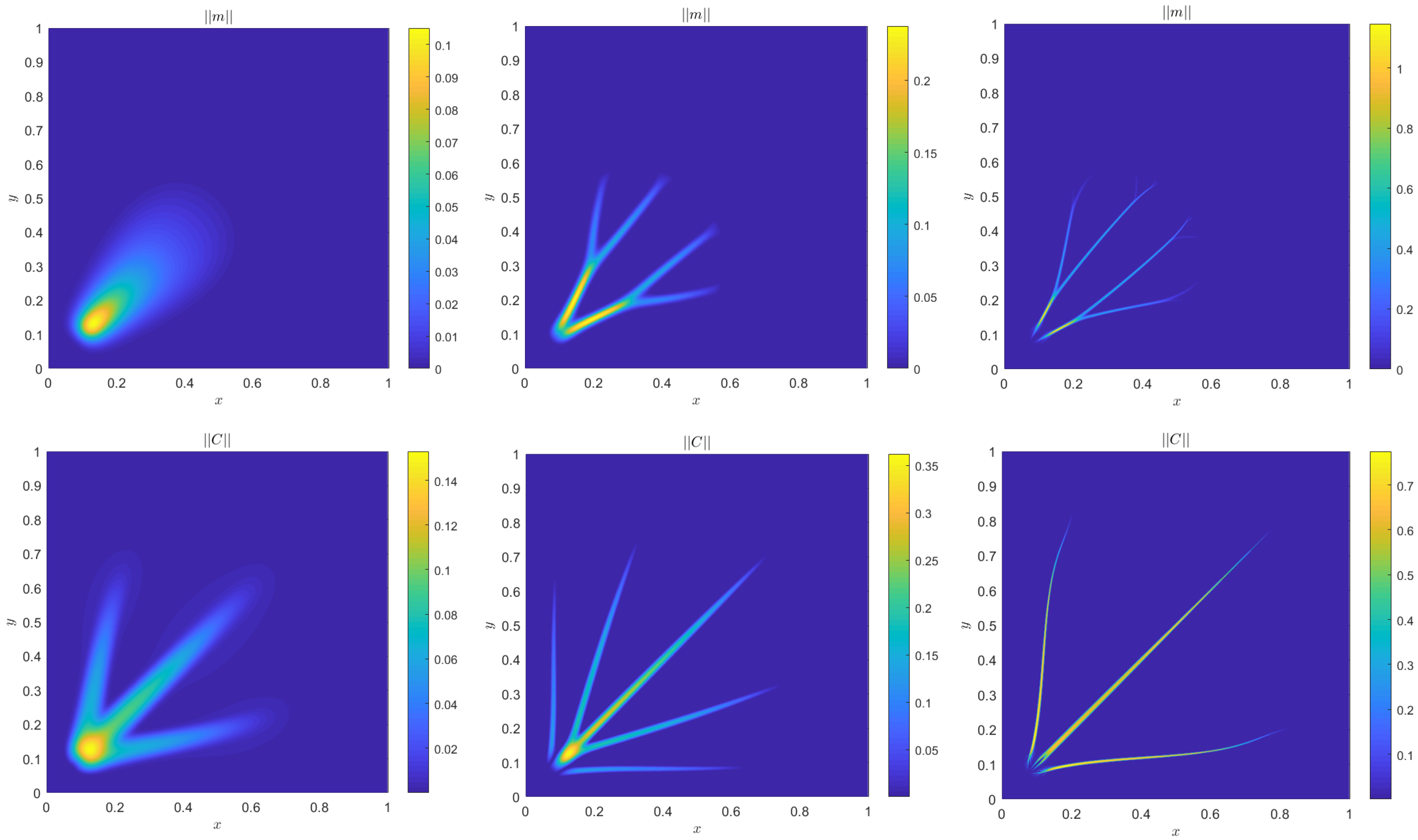
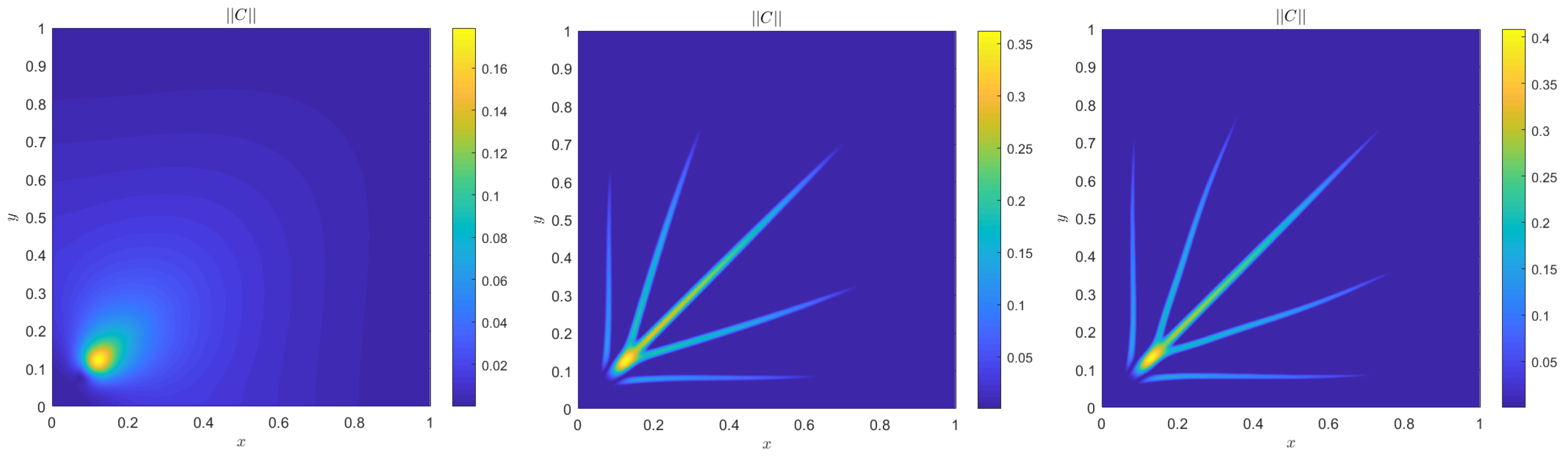
4. Numerical Results

In this section, we perform several simulations with the aim of studying the effect of the various parameters. In particular, we check the agreement of the two models for the m system in Equations (8) and (9) and for the $\mathbb{C}$ system in Equations (3) and (6).

4.1. Accuracy Tests and Qualitative Agreements

In

Table 1. In this table, we define all the tests that we show in Section 4.1. The first three rows show the parameters for the accuracy tests for m and $\mathbb{C}$, and the results are summarized in Table 2 and Table 3. The second three rows define the parameters that we use in Figure 2, where we compare the results of changing the diffusivity. The third three rows are the tests showed in Figure 3, varying $gamma$, and the results of the last three rows are in Figure 4, where we change the stabilization parameter $\epsilon$. For the accuracy tests, the number of points of the discretization is specified in Table 2 and Table 3, while for all the other tests, the number of points is fixed, and it is $N=600$.

		$\mathit{\alpha }$	c	D	$\mathit{\epsilon }$	$\mathit{\gamma }$	r	${\mathit{t}}_{\mathbf{fin}}$
Accuracy m	TestA:	0.5	1	0.01	-	0.75	0.1	1
Accuracy $\mathbb{C}$	TestB:	1	1	0.01	0.1	1.75	0.1	1
Accuracy m	TestC:	0.5	5	0.01	-	0.75	0.01	1
$D=0.05$	TestG:	0.75	5	0.05	${10}^{-3}$	0.75	0.005	15
$D=0.01$	TestD:	0.75	5	0.01	${10}^{-3}$	0.75	0.005	15
$D=0.001$	TestE:	0.75	5	0.001	${10}^{-3}$	0.75	0.005	15
$\gamma =1$	TestH:	0.75	5	0.01	${10}^{-3}$	1	0.005	15
$\gamma =0.75$	TestD:	0.75	5	0.01	${10}^{-3}$	0.75	0.005	15
$\gamma =0.5$	TestF:	0.75	5	0.01	${10}^{-3}$	0.5	0.005	15
$\epsilon ={10}^{-2}$	TestI:	0.75	5	0.01	${10}^{-2}$	0.75	0.005	15
$\epsilon ={10}^{-3}$	TestD:	0.75	5	0.01	${10}^{-3}$	0.75	0.005	15.
$\epsilon ={10}^{-4}$	TestL:	0.75	5	0.01	${10}^{-4}$	0.75	0.005	15

, we define the tests we want to show in this paper, varying the parameters of the systems. For this choice of parameters, a typical time scale is of the order of unit, while after time 15, the solution reaches the steady state.

First, we check the accuracy of the schemes adopted. In

Table 2. Accuracy test of the m system (8) and (9): we show the $L^2$-norm of the relative error for $\left|m\right|$, with the parameters defined in TestA (left) and TestC (right).

N	Error	Order	N	Error	Order
20	-	-	20	-	-
40	0.036030	-	40	0.036012	-
80	0.0492860	−0.4520	80	0.0493010	−0.4531
160	0.01454106	1.7610	160	0.01456192	1.7594
320	0.00690830	1.0737	320	0.00691103	1.0752
640	0.001529779	2.1750	640	0.001528055	2.1772

and

Table 3. Accuracy test of the $\mathbb{C}$ system (3) and (4): we show the $L^2$-norm of the relative error for $\left|\mathbb{C}\right|$, with the parameters defined in TestB.

N	Error${}_2$	Order
25	-	-
50	$9.066\times {10}^{-2}$	-
100	$4.625\times {10}^{-2}$	0.97
200	$1.571\times {10}^{-2}$	1.56
400	$4.149\times {10}^{-3}$	1.92
800	$7.347\times {10}^{-4}$	2.50

, we see the error for the conductivity variables, calculated with Richardson extrapolation (see, e.g., [13]). We show the error for the module of the vector and of the tensor, and the parameters chosen are defined in TestA, TestB and TestC.

Here, we define the initial conditions $m_{\mathrm{comp}}^0\left(\overrightarrow{x}\right)$ and ${\mathbb{C}}_{\mathrm{comp}}^0\left(\overrightarrow{x}\right)$, and the source function $S\left(\overrightarrow{x}\right)$

$$\begin{array}{cc}\hfill & m_{\mathrm{comp}}^0\left(\overrightarrow{x}\right)={[1,1]}^T,{\mathbb{C}}_{\mathrm{comp}}^0\left(\overrightarrow{x}\right)={[1,0,1]}^T,S\left(\overrightarrow{x}\right)=E-\overline{E}\end{array}$$

(29)

$$\begin{array}{cc}& E=exp(-\sigma {(\overrightarrow{x}-{\overrightarrow{x}}_0)}^2),\sigma =1000,{\overrightarrow{x}}_0=(0.1,0.1)\end{array}$$

(30)

where $\mathbb{I}$ is the identity matrix and $\overline{E}=\mathrm{mean}\left(E\right)$.

In Figure 1, we show three different quantities of TestD: the module of the variables at the final time (first column), the two components of the flux $|\mathbb{C}\nabla p|$ at the final time (second column) and the energy as a function of time (third column). In the first row, we have the results for the variable m, and in the second row, the results for the variable $\mathbb{C}$ are shown. As expected, the energy decays in time for both variables, and it is very small at the final time, which indicates that we are close to the steady state of the systems. The main difference between the two variables is the shape of the network, with a Y shape for the conductivity vector and a V shape for the tensor.

In Figure 2, we show the results obtained when varying parameter D in Equations (8) and (9) and in Equations (3)–(6). The tests we consider are: TestG (first column), TestD (second column) and TestE (third column), with $D\in \{0.05,0.01,0.001\}$ for variable m in the first row and for $\mathbb{C}$ in the second row. The ramifications become more evident when decreasing the diffusivity, and they become thinner and thinner. For the first parameter chosen, $D=0.05$, we are not able to see those ramifications for vector m because the time scale associated with the diffusion is too fast to capture the details.

In Figure 3, we observe the dependence on the relaxation exponent $\gamma$. In the first column, we report the results of TestH; in the second, those corresponding to TestD; and in the third one, those corresponding to TestF. Again, in the first row, we show the results for variable m, and in the second row, those for variable $\mathbb{C}$. If $\gamma =1$, the results do not show the details of the network, and it seems that $\gamma =0.75$ is the parameter that better represents the leaf network.

In Figure 4, we show the behavior of solution $\mathbb{C}$ when $\epsilon \to 0$. We see the results for $\epsilon \in \{{10}^{-2}\left(\mathrm{left}\right),{10}^{-3}\left(\mathrm{center}\right),{10}^{-4}\left(\mathrm{right}\right)\}$, and again, we notice that for the largest value of $\epsilon$, we are not able to see any ramification. Meanwhile, we see that for $\epsilon$ smaller than ${10}^{-3}$, we are close to asymptotic behavior.

4.2. Quantitative Agreement

In this section, we show some quantitative comparisons between the two models. For this reason, we consider well-prepared initial data, and we look for compatible parameters.

The goal of this part is to choose a convenient set of parameters in order to compare the two systems, trying to make them as close as possible. Now, we distinguish the parameters $(D_l,c_l,{\alpha }_l,{\gamma }_l)$ with $l=1$ for the $\mathbb{C}$ model, and $l=2$ for the m model.

For simplicity, the choice of parameter is performed by comparing the two models in one space dimension. In 1D, the systems (3), (6), (8) and (9) read

$$\begin{array}{cc}\hfill C_t-D_1^2{C}_{xx}-c_1^2{p}_x^2+{\alpha }_1{\left|C\right|}^{{\gamma }_1-2}C& =0\hfill \end{array}$$

(31)

$$\begin{array}{cc}\hfill m_t-D_2^2{m}_{xx}-c_2^2{p}_x^{2}m+{\alpha }_2{\left|m\right|}^{2({\gamma }_2-1)}m& =0.\hfill \end{array}$$

(32)

Now, we suppose that C has the following form:

$$C=m^2+B,$$

(33)

where B is a measure of the discrepancy between the two models, and we set the initial conditions so that $B(t=0)=0$. If we substitute Equation (33) in Equation (31), we have

$$\begin{array}{c}\hfill {\left(m^2\right)}_t-D_1^2{\left(m^2\right)}_{xx}-c_1^2{p}_x^2+{\alpha }_1|m^2{+B|}^{\gamma -2}{m}^2=-B_t+D_1^2{B}_{xx}-{\alpha }_1{|m^2+B|}^{\gamma -2}B.\end{array}$$

(34)

At this point, we multiply Equation (32) by a factor $\left(2m\right)$, and we obtain

$$2m{m}_t-2D_2^{2}m{m}_{xx}-2c_2^2{p}_x^2{m}^2+2{\alpha }_2{\left|m\right|}^{2({\gamma }_2-1)}{m}^2=0.$$

(35)

After some manipulation, Equations (34) and (35) become:

$$\begin{array}{ccc}\hfill & 2m{m}_t-D_1^2{\left(m^2\right)}_{xx}-c_1^2{p}_x^2+{\alpha }_1{\left(m^2\right)}^{\gamma -1}=\underset{:=\mathcal{R}}{\underbrace{-B_t+D_1^2{B}_{xx}-{\alpha }_1{\left|m^2\right|}^{\gamma -2}B}}& \end{array}$$

(36)

$$\begin{array}{cc}\hfill & 2m{m}_t-D_2^2{\left(m^2\right)}_{xx}+2D_2^2{\left(m_x\right)}^2-2c_2^2{p}_x^2{m}^2+2{\alpha }_2{\left(m^2\right)}^{{\gamma }_2}=0\end{array}$$

(37)

where $\mathcal{R}$ is the residual. We made use of the following identity in the equation for m

$${\left(m\right)}_{xx}^2=2m{m}_{xx}+2\left({\left(m_x\right)}^2\right).$$

(38)

Now, we consider the difference between Equations (36) and (37), and we obtain

$$(D_2^2-D_1^2){\left(m^2\right)}_{xx}-2D_2^2{\left(m_x\right)}^2+(2c_2^2{m}^2-c_1^2)p_x^2+{\alpha }_1{\left(m^2\right)}^{\gamma -1}-2{\alpha }_2{\left(m^2\right)}^{{\gamma }_2}=\mathcal{R}$$

(39)

Since we want the residual to be small, in absolute value, a convenient choice for the sets of variables is the following:

$$D_1=D_2,{\alpha }_1=2{\alpha }_2,{\gamma }_1={\gamma }_2+1,c_1=\sqrt{2}{c}_2\left|m\right|$$

(40)

and for the initial conditions, we choose $m^0$ and $C^0$ such that, initially, we have

$$C^0={\left(m^0\right)}^2=\mathrm{const}.$$

In this way, the first derivative in space $m_x$ is also equal to 0 after one time step.

In order to show some results in 2D, we need to define the initial conditions for $m_{\mathrm{comp}}^0$ and ${\mathbb{C}}_{\mathrm{comp}}^0$ such that, at the initial time, we have again

$${\mathbb{C}}^0=m^0\otimes m^0,$$

with $m_{\mathrm{comp}}^0={[\sqrt{2}/2,\sqrt{2}/2]}^T$ and ${\mathbb{C}}_{\mathrm{comp}}^0={[0.5,0.5,0.5]}^T$, while the values of the parameters are defined in TestM in

Table 4. In this table, we define the two sets of parameters in Equation (40).

		${\mathit{\alpha }}_1,{\mathit{\alpha }}_2$	${\mathit{c}}_1,{\mathit{c}}_2$	${\mathit{D}}_1={\mathit{D}}_2$	$\mathit{\epsilon }$	${\mathit{\gamma }}_1,{\mathit{\gamma }}_2$	r	N
set of parameters	TestM:	1, 0.5	$\sqrt{2}$, 1	0.1	${10}^{-1}$	1.75, 0.75	0.1	600

. In 2D, the equivalent expression of (33) is

$$\mathbb{C}=m\otimes m+\mathbb{B}.$$

In this subsection, we comment on the solutions of the following tests:

In

Table 5. Here, we show the values of $\mathbb{B}$, after $n_t$ time steps, where $n_t=2^k,k=0,1,2,3,4,5,6$.

Time	0.01	0.02	0.04	0.08	0.16	0.32	0.64
$\left|\right|\mathbb{B}\left|\right|$	0.0348	0.0538	0.0697	0.0982	0.1509	0.2611	0.5320

, we show the time evolution of the norm of the difference between $\mathbb{C}$ and $m\otimes m$, to see how they move away from each other when we increase the time. In this table, we see that the two solutions are very different, even after few time steps, and for this reason, they are difficult to compare. The definition of $\left|\right|\mathbb{B}\left|\right|$ is the following:

$$\left|\right|\mathbb{B}\left|\right|:=\frac{\left|\right|\left|\mathbb{C}\right|-|m\otimes m|\left|\right|}{\left|\right||m\otimes m|\left|\right|}$$

after $n_t$ time steps, with $\mathrm{time}=n_t\Delta t$, such that $n_t=6\left(2^k\right),k=0,1,2,3,4,5,6$, where $\left|\mathbb{C}\right|:=\sqrt{{\mathbb{C}}_{11}^2+2{\mathbb{C}}_{12}^2+{\mathbb{C}}_{22}^2}$ and $|m\otimes m|:=\sqrt{{\left(m_1^2\right)}^2+2{\left(m_1{m}_2\right)}^2+{\left(m_2^2\right)}^2}$.

As it appears from the table, the two models move quickly far apart from each other, suggesting intrinsically different behavior.

Now, we are interested in showing the solution of the $\mathbb{C}$ model, in the case of zero-diffusivity. Since the randomness of the network is common in nature but is also very effective in stabilizing the equations, we want to see if there is some analogy in considering the cases $D=0$ and $D\ll 1$. We call ${\mathbb{C}}_{\left(D\right)}$ the solution with $D={10}^{-5}$ and ${\mathbb{C}}_{\left(0\right)}$ when $D=0$. In Figure 5, we show the agreement of the two solutions, with $D=0$ (left panel) and $D={10}^{-5}$ (right panel). The other parameters are defined in TestN and TestO in

Table 6. In this table, we define the two tests showed in Figure 5 and Figure 6, with $D=0$ (TestN) and $D={10}^{-5}$ (TestO).

		$\mathit{\alpha }$	c	D	$\mathit{\epsilon }$	$\mathit{\gamma }$	r	${\mathit{t}}_{\mathbf{fin}}$	N
$D=0$	TestN:	0.75	5	0	${10}^{-3}$	0.75	0.005	15	600
$D={10}^{-5}$	TestO:	0.75	5	${10}^{-5}$	${10}^{-3}$	0.75	0.005	15	600

, while the initial condition is defined in Equation (29) for Figure 5.

In Figure 6, we illustrate the long time solution for the $\mathbb{C}$ model obtained with the following space-dependent initial condition:

$${\mathbb{C}}^0=f(x,y)\mathbb{I},f(x,y)=(2-|X+Y\left|\right)exp(-10(|X-Y|\left)\right)$$

(41)

In order to show some quantitative comparison between the results, we calculate the difference in the solutions, at the final time, with the following expression:

$$\mathrm{diff}=\frac{\left|\right||{\mathbb{C}}_{\left(D\right)}|-|{\mathbb{C}}_{\left(0\right)}\left|\right||}{\left|\right||{\mathbb{C}}_{\left(0\right)}\left|\right||}.$$

This value, for the comparison shown in Figure 5, is $\mathrm{diff}=4.81\times {10}^{-3}$, and that for Figure 6 is $\mathrm{diff}=2.37\times {10}^{-4}$. If we consider that the spatial step is $\Delta x=1.66\times {10}^{-3}$, the resulting values of this difference are not surprising because they are both of the order of $\Delta x$.

As we explain in the Section 2, the Dirichlet integral is important to describe the randomness of the network, and it is essential for the ${\mathcal{E}}_{\mathrm{vect}}\left[m\right]$, because, without that term, there is no network formation for the m model. In particular, if the initial condition for m has a support ${\Omega }_0\subset \Omega$, there is no mechanism that extends the support, since m will remain a zero vector in the whole $\Omega \setminus {\Omega }_0$. From the analytical point of view, it is also necessary to regularize the model, and this is the main reason why we have a diffusion term (with $D\ne 0$), coming from the gradient flow of that Dirichlet integral.

We also note that, if we set the diffusion coefficient equal to zero, the model for m reduces to a reaction equation for the conductivity. This means that if $\gamma >1/2$, the support of the unknown m remains unchanged. In particular, it cannot extend, while in some regions, the numerical support (i.e., the region in which $\left|m\right|$ becomes lower than a given small threshold) may shrink.

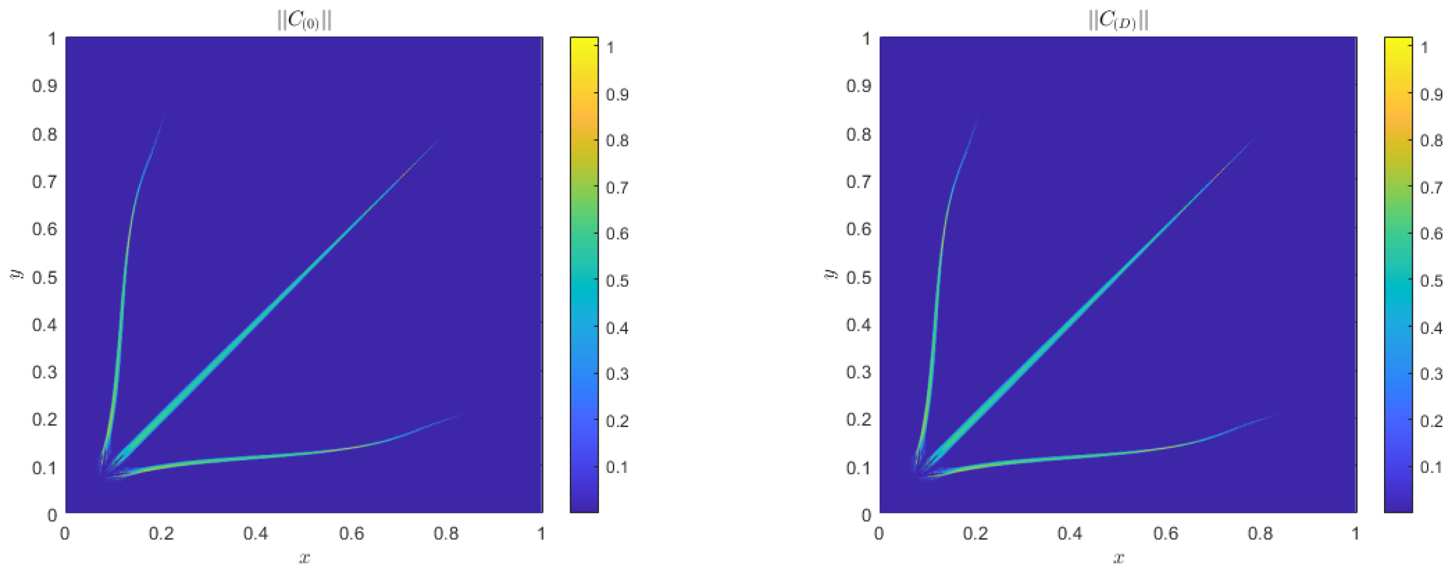
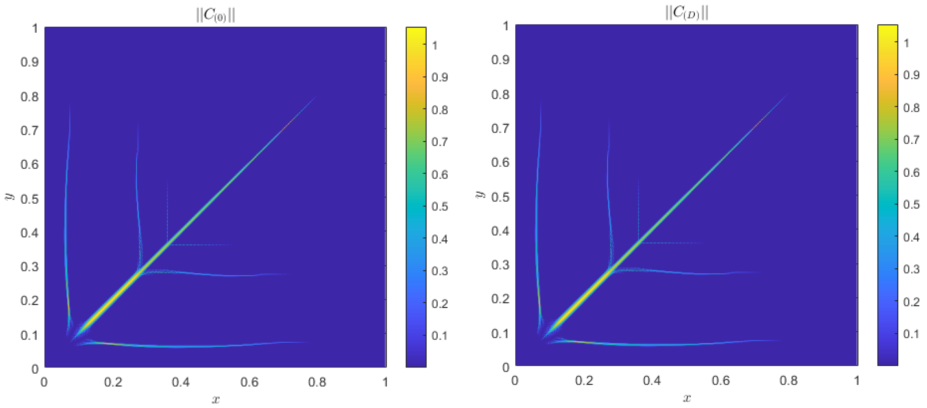
Alternative Boundary Conditions

Furthermore, in the case of zero-diffusivity for the m model, we observe anomalous behavior of the solution near the boundaries. In order to overcome such a problem, we propose an ad hoc boundary condition as illustrated below.

Let us consider the equations for m with $D=0$ and in the limit of steady state. We have

$$\begin{array}{cc}\hfill c^2\nabla p\otimes \nabla pm-\alpha {\left|m\right|}^{2(\gamma -1)}m& =0\mathrm{in}\partial \Omega \hfill \end{array}$$

which we can write as follows:

$$\begin{array}{c}\hfill (m·\nabla p)\nabla p=\frac{\alpha }{c^2}{\left|m\right|}^{2(\gamma -1)}m\mathrm{in}\partial \Omega \end{array}$$

(42)

Thus, we can deduce that $m\propto \nabla p$. This means that there exists a constant $\beta$, such that,

$$m=\beta \nabla p.$$

(43)

If we substitute Equation (43) in Equation (42), we obtain

$${\beta |\nabla p|}^2\nabla p=\frac{\alpha }{c^2}{\beta }^{2(\gamma -1)}{|\nabla p|}^{2(\gamma -1)}\beta \nabla p$$

(44)

and if we solve it for $\beta$, we have the boundary condition for m

$$\begin{array}{c}\hfill {\left.m\right|}_{\partial \Omega }=\underset{\beta }{\underbrace{{\left(\frac{c^2}{\alpha }{|\nabla p|}^{4-2\gamma }\right)}^{\frac{1}{2(\gamma -1)}}}}\nabla p.\end{array}$$

(45)

Analogously, we can also find a boundary condition for vector $\mathbb{C}$. Again, starting with zero-diffusivity and at steady state, we have

$$\nabla p\otimes \nabla p=\frac{\alpha }{c^2}{\left|\mathbb{C}\right|}^{\gamma -2}\mathbb{C}\mathrm{in}\partial \Omega$$

(46)

which means that the conductivity is proportional to the tensor product of the pressure gradient, i.e., $\mathbb{C}\propto \nabla p\otimes \nabla p$. Again, we look for a constant $\tilde{\beta }$, such that,

$$\mathbb{C}=\tilde{\beta }\nabla p\otimes \nabla p.$$

(47)

Now, we substitute Equation (47) in Equation (46), and we solve this for $\tilde{\beta }$. In this way, as before, we find the expression for the conductivity tensor at the boundary

$${\left.\mathbb{C}\right|}_{\partial \Omega }=\underset{\tilde{\beta }}{\underbrace{{\left(\frac{c^2}{\alpha }{|\nabla p|}^{-2(\gamma -2)}\right)}^{\frac{1}{\gamma -1}}}}\nabla p\otimes \nabla p.$$

(48)

Conditions (45) and (48) might be a reasonable choice in the case of zero diffusivity. This treatment has the drawback of introducing additional non-linearity to the system. Alternative boundary conditions are currently under investigation.

Another aspect we want to focus on is the steady state for the m model in two different cases: $\gamma <1$ and $\gamma >1$ (as the authors show in [7]). For this reason, we define different initial conditions for the vector m, such that

$$\begin{array}{ccc}& m_1^{0,1}=1,m_2^{0,1}=\sqrt{2};m_1^{0,2}=5,m_2^{0,2}=5;& \\ & m_1^{0,3}=(2-|X+Y\left|\right)exp(-10|X-Y\left|\right),m_2^{0,3}=m_1^{0,3};\end{array}$$

and in Figure 7, we plot the following quantity:

$$\mathrm{diff}=\frac{\left|\right|m^{\beta }-m^{\eta }\left|\right|}{\left|\right|m^{\eta }\left|\right|}$$

(49)

where $\left|\right|·\left|\right|$ is the Frobenius norm, and $\beta ,\eta \in \{1,2,3\}$. In this way, we see the difference between the solutions (with the initial condition $m^{0,1}$ and $m^{0,2}$ in the left panel and with $m^{0,1}$ and $m^{0,3}$ in the right panel) as a function of time. In this way, we support with numerical evidence that, for the m model and for $\gamma >1$, the steady state is unique and it does not depend on the initial conditions, as expected (see e.g., [7]).

In Figure 8, which is the case for $\gamma <1$, we see that we reach two different steady states when choosing two different initial conditions, suggesting that the steady state solution is not unique when $\gamma <1$.

5. Conclusions

In this paper, we use an elliptic–parabolic model to study the formation of a biological network, and, in particular, of leaf venation networks. Throughout the paper, we compare the solutions of two different systems, which derive from the Cai–Hu model, one for the conductivity vector and one for the conductivity tensor, and we explore the dependence of the solution on the parameters of the two models.

As we said before, all the components of the two systems are very stiff. In particular, the $\mathbb{C}$ system is more challenging because of the negative exponent in the reaction term. For this reason, we add a regularization parameter $\epsilon$, and we compute numerical solutions for smaller and smaller values of $\epsilon$. This parameter prevents the instability coming from the division by zero in the reaction term.

We make use of the finite differences scheme to compute the two solutions, with central differences for the space discretization and a symmetric ADI method in time. The convergence rate is calculated numerically and denotes the second-order accuracy.

At the end, we add some quantitative comparisons between the two systems, choosing more suitable sets of parameters. We see that the two solutions differ significantly, even after few time steps. This aspect makes any kind of direct comparison between the two systems problematic.

Then, we show some results in the case of zero diffusivity for the conductivity tensor. The last tests we consider in this paper are in agreement with the results achieved in [7], where the authors prove that there is a unique steady state for the m system when the metabolic exponent $\gamma$ is greater than 1 and provide evidence that indeed this is not true when $\gamma <1$.

References

1. Hu, D.; Cai, D. Adaptation and optimization of biological transport networks. Phys. Rev. Lett. 2013, 111, 138701. [Google Scholar] [CrossRef] [PubMed]
2. Katifori, E.; Szöllosi, G.J.; Magnasco, M.O. Damage and fluctuations induce loops in optimal transport networks. Phys. Rev. Lett. 2010, 104, 048704. [Google Scholar] [CrossRef] [PubMed] [Green Version]
3. Hu, D.; Cai, D. An optimization principle for initiation and adaptation of biological transport networks. Commun. Math. Sci. 2019, 17, 1427–1436. [Google Scholar] [CrossRef]
4. Darcy, H. Les Fontaines Publiques de la Ville de Dijon: Exposition et Application des Principes à Suivre et des Formules à Employer Dans les Questions de Distribution d’eau: Ouvrage Terminé par un Appendice Relatif aux Fournitures d’eau de Plusieurs Villes, au Filtrage des Eaux et à la Fabrication des Tuyaux de Fonte, de Plomb, de tôle et de Bitume; Dalmont, V., Ed.; Typographie Hennuyer: Paris, France, 1856. [Google Scholar]
5. Neuman, S.P. Theoretical derivation of Darcy’s law. Acta Mech. 1977, 25, 153–170. [Google Scholar] [CrossRef]
6. Fang, D.; Jin, S.; Markowich, P.; Perthame, B. Implicit and Semi-implicit Numerical Schemes for the Gradient Flow of the Formation of Biological Transport Networks. SMAI J. Comput. Math. 2019, 5, 229–249. [Google Scholar] [CrossRef]
7. Haskovec, J.; Markowich, P.; Perthame, B. Mathematical Analysis of a PDE System for Biological Network Formation. Commun. Partial. Differ. Equ. 2015, 40, 918–956. [Google Scholar] [CrossRef] [Green Version]
8. Haskovec, J.; Markowich, P.; Perthame, B.; Schlottbom, M. Notes on a PDE system for biological network formation. Nonlinear Anal. 2016, 138, 127–155. [Google Scholar] [CrossRef] [Green Version]
9. Albi, G.; Artina, M.; Foransier, M.; Markowich, P.A. Biological transportation networks: Modeling and simulation. Anal. Appl. 2016, 14, 185–206. [Google Scholar] [CrossRef]
10. Haskovec, J.; Markowich, P.; Portaro, S. Emergence of biological transportation networks as a self-regulated process. arXiv 2022, arXiv:2207.03542. [Google Scholar]
11. Haskovec, J.; Markowich, P.; Pilli, G. Tensor PDE model of biological network formation. Commun. Math. Sci. 2022, 20, 1173–1191. [Google Scholar] [CrossRef]
12. Wesseling, P. Principles of Computational Fluid Dynamics; Springer: Berlin/Heidelberg, Germany, 2001. [Google Scholar]
13. Richardson, L.F. IX. The approximate arithmetical solution by finite differences of physical problems involving differential equations, with an application to the stresses in a masonry dam. Philos. Trans. R. Soc. Lond. Ser. A Contain. Pap. Math. Phys. Character 1911, 210, 307–357. [Google Scholar]
Figure 1. In this figure, we show three different quantities of the same computations, with the parameters defined in TestD: the module of the variables at final time (left panels), the flux also at final time (central panels) and the energy as a function of time (right panels). The first row concerns variable m, and the second one is for variable C .
Mca 27 00087 g001
Figure 2. In this figure, we show the difference in the results on varying the diffusivity D. In the first column, we have the results of TestG ( D = 0.05 ); in the second column, we choose the parameters of TestD ( D = 0.01 ), and in the third one, TestE ( D = 0.001 ). The first row shows the results of variable m, and the second row shows those of variable C .
Mca 27 00087 g002
Figure 3. In this figure, we show the difference in the results on varying the relaxation exponent γ . In the first column, we have the results of TestH ( γ = 1); in the second column, we choose the parameters of TestD ( γ = 0.75 ); and in the third one, TestF ( γ = 0.5 ). The first row shows the results of variable m, and the second row, variable C .
Mca 27 00087 g003
Figure 4. In this figure, we show the results for variable C varying the parameter ε . On the left, we have the results of TestI ( ε = 10 2 ), in the central panel, TestD ( ε = 10 3 ) , and on the right, TestL ( ε = 10 4 ) .
Mca 27 00087 g004
Figure 5. Comparison between TestN and TestO, with initial condition defined in Equation (29). The main difference is that on the left, we have D = 0 , while on the right, we have D = 10 5 .
Mca 27 00087 g005
Figure 6. Comparison between TestN and TestO. Here, the initial condition is defined in Equation (41), with D = 0 on the left and D = 10 5 on the right.
Mca 27 00087 g006
Figure 7. In this figure, we show the difference between two different solutions choosing, as initial conditions, m 0 , 1 , m 0 , 2 (left) and m 0 , 1 , m 0 , 3 (right). We plot the expression defined in Equation (49) as a function of time, with γ = 1.75 > 1 , and the others parameters are defined in TestD.
Mca 27 00087 g007
Figure 8. In this figure, we show the steady states when γ = 0.75 < 1 . On the left, the initial condition is m 0 = m 0 , 1 = 1 while on the right, the initial condition is a function of space, m 0 = m 0 , 3 , and the parameters are defined in TestD.
Mca 27 00087 g008