1. Introduction
Often, engineers and scientists may need to choose a software that is specific to their application or modeling purpose. Some software languages may have different features, speed/computational complexity, tolerances, architecture, libraries, ease of use, etc., that can affect the accuracy of the model. Here, we investigated the performance of the mathematical software program Maple and the programming language MATLAB when applying the method of steps (MoS) and the Laplace transform (LT) methods to solve linear delay differential equations (DDEs). To make the comparison fair, we used the benefits offered by these two programs for symbolic computation, which allows us to derive the solutions of these DDEs in the ways we would think about carrying them out by hand with variables, symbols, functions, and other mathematical formulas. An advantage of using symbolic computation is that it eliminates cases of roundoff errors in intermediate calculations since parameter variables are carried throughout the calculations using infinite precision arithmetic [
1,
2,
3]. However, in some cases, using symbolic computations can lead to slower execution times depending on the program used and the process [
4,
5,
6]. Symbolic computation has been used and proposed for solving many different problems [
7,
8,
9,
10,
11].
In this paper, we focus on comparing the symbolic mathematical computations of Maple and MATLAB to obtain analytical solutions of linear neutral and non-neutral DDEs by using the LT method. The accuracy of the LT solutions may be determined by comparing them with the MoS solutions [
12,
13,
14,
15,
16,
17]. However, the MoS has a very important limitation since it is a stepwise process that requires solving the relevant differential equation in each respective time interval, which can be computationally expensive. Moreover, for many types of DDEs, we will often encounter the swelling phenomena, i.e., the complexity of the closed-form solution increases rapidly in each successive time interval, making the computations unfeasible [
14,
16]. On the other hand, the LT method produces a solution that can be evaluated at any particular value of time. Thus, we can compute the approximated solution by evaluating it at any point. Other advantages of the analytical solutions, such as the long-term behavior of the solution, can be seen in [
14,
15,
18,
19,
20,
21,
22]. The errors of the LT solutions usually decrease as time increases. On the other hand, for classical numerical solutions, the computation increases as
[
14,
23,
24,
25]. However, numerical schemes that solve linear and nonlinear DDEs are useful and, in some cases, are easy to implement. For instance, in [
26], the authors developed a numerical scheme based on a fitted difference scheme with the use of exponential basis functions and interpolating quadrature rules to solve first order linear DDEs. Some researchers have proposed different collocation methods to solve linear and nonlinear DDEs [
27,
28]. For instance, in [
29], the Haar wavelet collocation method was applied to obtain the numerical solution of a particular class of DDEs. The method is also applied to systems involving DDEs. In [
30], the authors proposed a numerical method for solving linear fractional differential equations using discretization at the Jacobi–Gauss collocation points. Other methods that have been applied that involve more general DDEs can be found in [
31,
32]. In these works, the authors deal with the differential-difference equation in an infinite-dimensional space and with unbounded domains. Moreover, they consider mixed-type equations that include both forward and backward shifts of the argument. These forms are generated by different temporal and spatial discretizations. It is important to mention that one might expect that some of the techniques and results of retarded differential equations could be applied to mixed-type equations, but, given that the independent variable in this paper is strictly temporal, this may require one to introduce some modifications [
32,
33]. In addition, these last works deal with idealized nonlinearities in order to obtain a more tractable problem.
It is important to point out that, even for linear DDEs, it might be challenging to obtain an analytical solution. Moreover, in most cases, the neutral delay differential equations (NDDEs) are more difficult to solve due to the appearance of a time delay on the derivative of the state variable. Regarding solving ordinary differential equations (ODEs) and DDEs, the latter is usually more difficult to solve since the derivatives of the state variables depend on the values of the state variable from the past. The classic approach used to obtain the solutions of DDEs is the MoS, but, in many cases, it is unfeasible to advance further in time and obtain the solution in the long term [
14,
15,
34,
35,
36]. In [
14], the authors studied the accuracy of the LT for linear DDEs and, in particular, for NDDEs. In [
20], the authors developed a method for solving linear and nonlinear DDEs with a proportional delay using a combination of the LT and the differential transformation method (DTM). The authors mentioned that the convergence rate can be improved by the combination of the two methods. The LT method has also been used to solve linear second order DDEs [
37]. However, complex analytical computations and the use of the residue theorem are required [
14,
37]. Linear DDEs have different applications and have been applied in many problems [
17,
38,
39].
In order to compare the symbolic computations involved in obtaining the solutions of neutral and non-neutral linear DDEs using the LT method, we selected Maple and MATLAB software since they are well-known in the scientific community [
3,
40]. In Maple, we made use of the symbolic functions
diff,
dsolve,
fsolve,
eval, and
subs, to name a few, whereas, in MATLAB, we utilized functions from the symbolic math and optimization toolboxes such as
fsolve,
subs,
vpa, and
vpasolve. We explored several examples of DDEs of neutral and non-neutral type in order to compare the symbolic computation of Maple and MATLAB. For each example, we computed the solution over some finite time interval using the MoS briefly described in
Section 2.1 and the LT method described in
Section 3. First, we explored two examples of non-neutral DDEs and then we followed with several examples of neutral DDEs. For each example, we compared: (1) the solutions of the two methods from each program software, (2) the errors associated with each method and software, and (3) the computation times. DDEs have been used in many different fields, including astronomy and epidemiology [
17,
41,
42,
43]. For some applications, such as control or communication systems, the computation time may be a critical factor [
44,
45,
46,
47]. All computations were performed on a computer system with an Intel(R) Core(TM) i9-10900K CPU @ 3.70 GHz processor and 64 GB RAM.
The organization of this paper is as follows. In
Section 2, preliminaries for DDEs, NDDEs, and the MoS for solving linear DDEs are presented. In
Section 3, we briefly present the main aspects of the LT method with the relevant equations and formulas. In
Section 4, we compare the symbolic computations to obtain the solution of linear DDEs using the LT method. We present several examples related to DDEs and their corresponding numerical solutions. In
Section 5, conclusions regarding the symbolic computations required to obtain the solution of DDEs using the LT method are provided.
2. Preliminaries
In this section, we present some preliminary definitions that are needed to solve the different linear DDEs presented in this work. Some preliminaries include background concepts, the Lambert function, the residue theorem, and the MoS. Familiarity with the basic concepts of complex analysis is assumed.
2.1. Method of Steps (MoS)
The traditional method for solving DDEs is with an elementary method called the method of steps [
17,
34,
35,
48,
49,
50]. It is well-known for being a tedious process when being worked out by hand, but the complexity can be drastically simplified with symbolic toolboxes in computer programs [
15]. Let us consider a NDDE with fixed delay
:
where
is the initial time value,
is a constant/discrete delay, and
is some constant. For DDE initial value problems (IVPs), we require a
history function,
, and an initial value,
for
, to solve the problem. This condition implies that DDEs are in fact infinite-dimensional problems since we define an infinite set of initial conditions between
.
Using integration properties on the interval
, the solution is then given by
, which is a solution to the following NDDE:
Repeating this process for successive intervals and using the solution over the past interval, we find the following general derivative formula for the
nth partition of the IVP (
):
The solutions of
form a piecewise solution of the original NDDE (
1) on the interval
.
Even though the MoS provides an analytical solution for DDEs, it has some drawbacks, including time consumption and the complexity of the integrals to be solved over each interval. This method also requires full knowledge of the history before the approach can be used. Since it is a successive process, it can be quite difficult to observe the behavior of the solution or to perform stability analysis of as .
2.2. Lambert W Function
From ODEs, the roots of the characteristic equation provide information about the solution of a linear ODE or system of linear ODEs. Often times, this equation is a simple polynomial that is easy to solve with algebraic operations or use of the quadratic formula. A linear DDE or system of linear DDEs can be characterized in a similar manner to ODEs by looking at the characteristic equation. Take, for example, the following linear DDE with discrete time delay
:
where
is the initial value. The characteristic polynomial of the above DDE takes the form of a quasi-polynomial due to the introduction of the exponential, i.e.,
. By setting
, there could be an infinite number of poles. Through simplifying, we obtain
, which takes the form of a
Lambert W function with the equation form
, where
z is some complex number and
is the multi-valued function solution of the equation.
Lambert functions are used when the unknown of an equation appears as both a base and exponent. Equations such as cannot be solved with algebraic, logarithmic, or exponential properties. For certain values of z, this equation can have an infinite number of solutions called branches of W, and are denoted by for . One of the branches, called the principal branch, is analytic at zero and is denoted by (). For real numbers, the branches and can be used to solve the equation with real numbers x and y if . The solution, y, can be found using the following conditions.
We note that the second condition implies that, in the interval , the equation has two real solutions.
In terms of our given problem, the poles of the quasi-polynomial are given by
. The analytical solution to the DDE, then, can be expressed in terms of an infinite number of branches, given as
where the
s are the coefficients determined from the history function,
, and the initial value,
. One can analyze how changes in the parameters
c,
, and
affect the real part of the eigenvalues of the system and, in turn, how that impacts the stability of the solution. Further details and applications of the Lambert function can be found in literature such as [
51,
52].
2.3. Cauchy’s Residue Theorem
The LT method for solving DDEs requires the use of Cauchy’s residue theorem, which is a powerful tool discussed in complex analysis for evaluating complex real integrals or infinite series [
53,
54]. Here, it was used to find the solution of a DDE when converting from the
s-space back to the
t-domain.
Suppose
is an analytic function in the complex region
defined by
, or the neighborhood of a point
. Then,
is an
isolated singular point of
. The function
can be represented by the Laurent series expansion as [
54]:
where
are the coefficients and
C is a simple closed contour in
. The
principal part of the series is given by the negative portion,
, where
is called the
residue of
at
. An isolated singularity is a
pole if
is of the form [
53,
54]:
where
is the order of the pole,
is an analytic function in
, and
.
Residues of Poles: If
, then
has a
simple pole at
. At a simple pole
, the residue of
is given by [
54]:
If the limit does not exist, then there exists an essential singularity at
. If the limit is zero, then
is analytic at
, or
is a removable singularity. If the limit is infinity, then the order is greater than
[
53,
54].
Now, suppose
can be expressed as a rational function,
, where
and
are analytic functions in
and
has a zero at
. Let
, where
is analytic in
and
is nonzero. Using the Taylor series expansion of
and
, the residue is given as [
53,
54]:
If
, then
has a pole of order
M at
. From Equation (
2), the residue of
at
is given by [
53,
54]:
Residue Theorem: Suppose
C is a simple closed contour and let
be an analytic function inside and on
C, excluding a finite number (
K) of isolated singularities inside
C. Then,
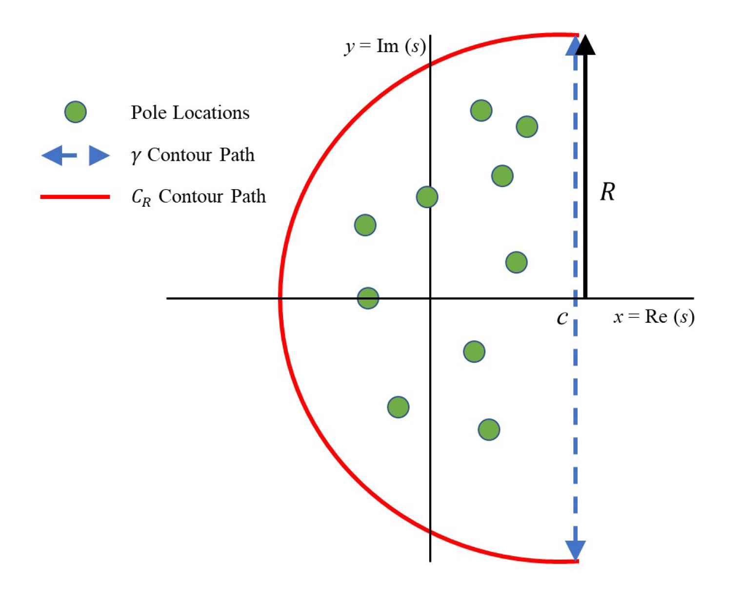
The use of Cauchy’s residue theorem in the LT method comes from the definition of the inverse Laplace transform (ILT):
where the integration is over a vertical path in the complex plane defined at
Re
. From complex analysis, the function
is entire and, thus, we require the vertical path to be to the right of all of the poles of
. In other words, the real part of all of the poles needs to be to the left of
c. Let us denote this vertical path
shown in
Figure 1. To use the residue theorem to evaluate the above integral, we construct a contour path,
, enclosing all of the poles with radius
R as shown in
Figure 1 going in a CCW direction. From this contour and Cauchy’s residue theorem, we obtain
which implies that
Let
. We need to show that
. Achieving this will give:
where
c is a fixed real constant s.t.
has a finite number of poles located to the left of the line
.
Let
. For
, we enclosed in the left half plane where
,
. Then,
, and we obtain
We find that
and
for sufficiently large
. Then, we have
In the integrand, we note that
is negative for
. Then, as
, we can observe that
, which implies that
. Then, we have shown that the ILT of
can be represented using residues and is given by
4. Comparison of MoS and LT Methods Using Symbolic Computation
Here, we present and discuss different examples of non-neutral DDEs and NDDEs introduced in [
14] and apply the MoS and LT methodologies to each example to find the solution of such equations using the Maple and MATLAB software. First, the solutions obtained by each method will be compared between programs to highlight the variances in program computations. Second, the accuracy of the LT method will be evaluated against the analytical solution obtained by the MoS for each program. For this section, we introduce the following notation:
: Absolute error in the solution between Maple and MATLAB via the MoS.
: Absolute error in the solution between Maple and MATLAB via the LT.
: Absolute error in the solution between the MoS and LT via Maple.
: Absolute error in the solution between the MoS and LT via MATLAB.
4.1. Linear Non-Neutral DDE Examples
The two examples presented in this section demonstrate solutions formed from poles of order
.
Figure 2 and
Figure 3 and
Table 1 summarize the solution results, error comparisons between MoS and LT in each programming language, and the computation times for the corresponding example.
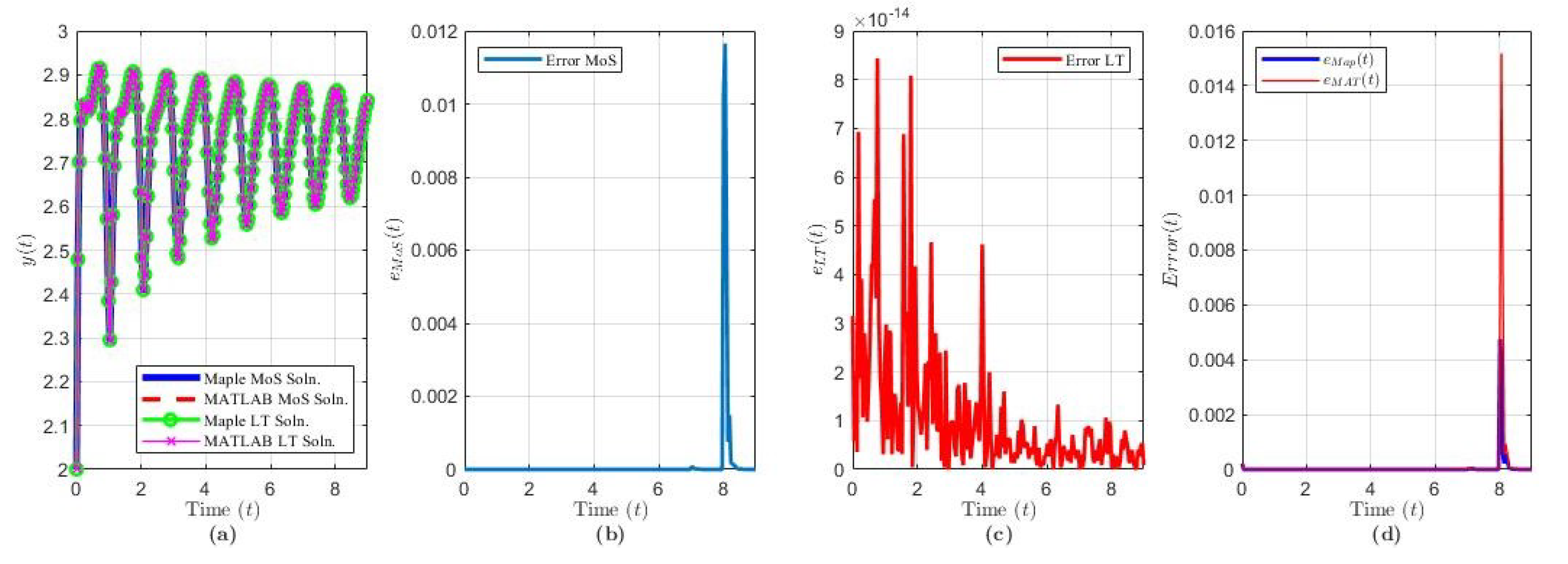
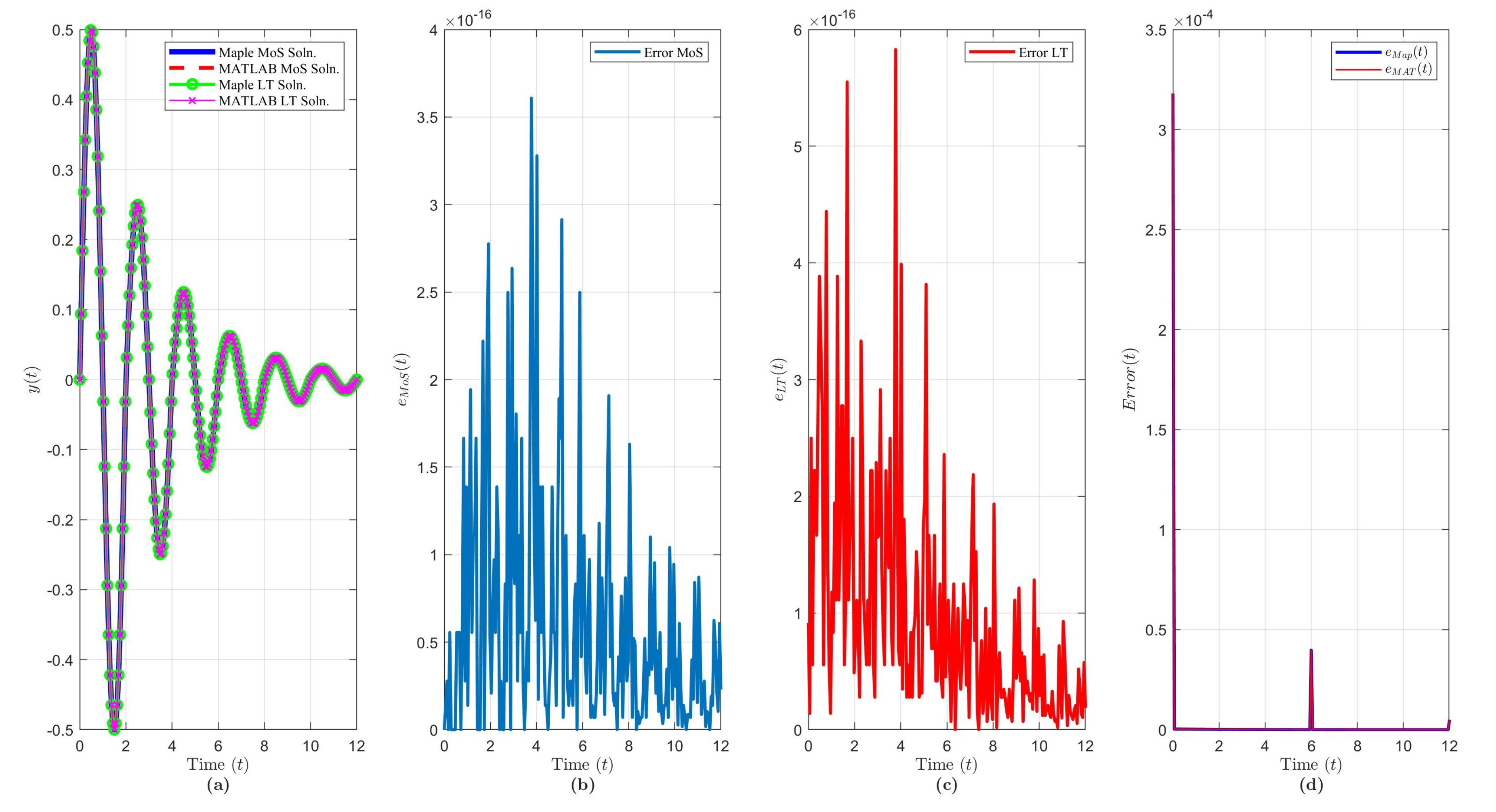
Example 1. Let us consider the following DDE:where . Taking the LT of Equation (19), we obtain the quasi-polynomial , which has a real pole at with residue (from Equation (4)). The remaining poles and residues are given by: , , with property , and . Applying the ILT and Cauchy’s residue theorem, we obtain the LT solution of : The solution of Example 1 via MoS (over
intervals) and LT (
) and in each software program is shown in
Figure 2a. We notice that, as
,
since
,
, and each Re
for
.
Figure 2b,c demonstrate the variances between the software when evaluating the solution via MoS (blue curve) or the LT (red curve).
Figure 2d demonstrates the accuracy of the LT compared to the analytical MoS via Maple (blue curve) and MATLAB (red curve). Upon analyzing
Figure 2b,d, we note that the MATLAB MoS solution significantly deviates from its LT solution and the Maple MoS solution. In the MoS process, a piecewise function is produced for each interval and it becomes harder to integrate and solve the sub-IVPs as the functions become more complicated with each step. In the LT solution, we see that, as
t progresses, the variance fluctuations in the solution between programs decrease. Each plot shows that error spikes occur every
. The reason is that, around these points, the sines of the truncated non-harmonic series do not play any significant role, while the cosine and exponential terms are essentially equal to 1. Therefore, the approximated series solution loses the ability to approximate the solution close to
. The spikes can be reduced if we include more terms in the truncated series [
14].
The computation times via each method and software are shown in
Table 1. Given the number of terms to compute for the LT solution, the computation time was higher for both programs compared to the MoS solutions. However, with the use of MATLAB’s symbolic toolbox functions, the computation time for the LT solution was reduced by a factor of four compared to Maple for this particular example.
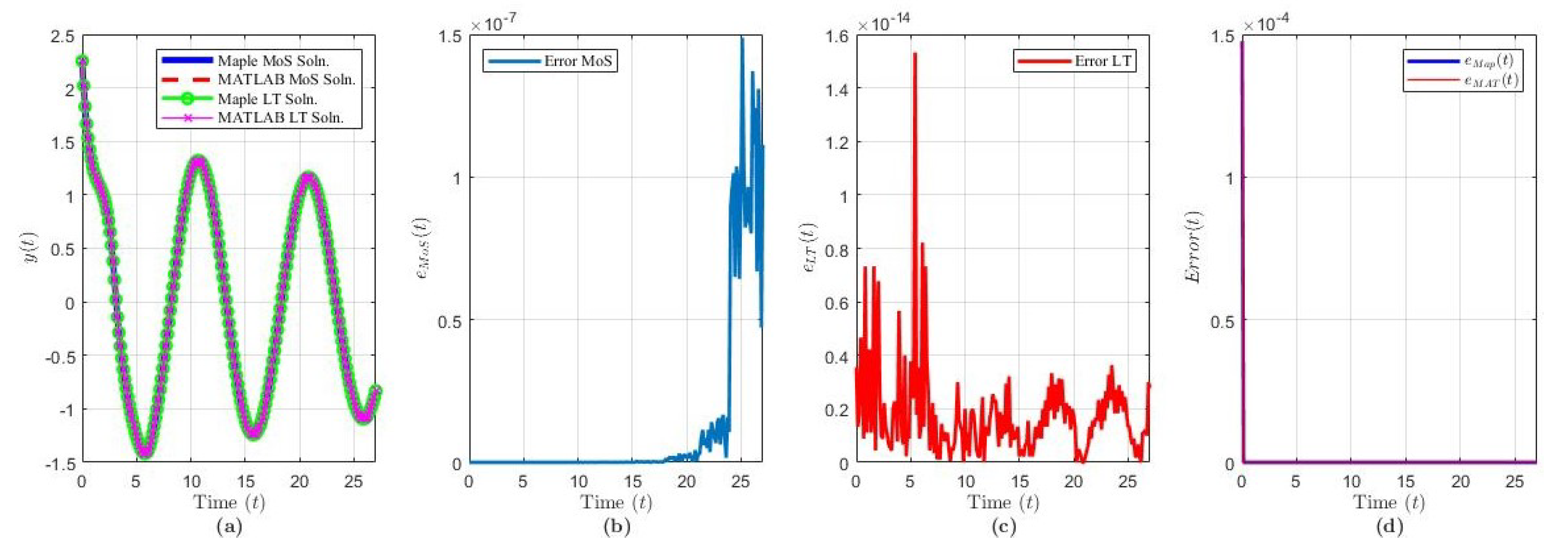
Example 2. Let us consider the following DDE:where . Taking the LT of Equation (20), we obtained the quasi-polynomial , which has no real poles since (see [14]). The complex poles are given by: , , with property , and corresponding residues . Applying the ILT and Cauchy’s residue theorem, we obtained the LT solution of : The solution of Example 2 via MoS (over
intervals) and LT (
) and in each software program is shown in
Figure 3a. We noticed that, as
,
since Re
.
Figure 3b,c demonstrates the variances between the software when evaluating the solution via MoS (blue curve) or the LT (red curve).
Figure 3d demonstrates the accuracy of the LT compared to the analytical MoS via Maple (blue curve) and MATLAB (red curve).
Compared to Example 1,
Figure 3b,d demonstrates that the performance error in MATLAB’s MoS solution, relative to the Maple MoS solution and the MATLAB LT solution, decreased. One notable difference between Examples 1 and 2 is the reduced complexity in the history function. In Example 1, the history function was a fifth-order polynomial, whereas, here, the history is a second-order polynomial. In both examples, the LT solution is truncated to 5000 terms. Note that truncation creates ringing in the solution near the history function endpoints. In
Figure 3d, the LT error decreases exponentially for both software, while, in
Figure 2d, we notice that the error has a maximum peak at around
. In some cases, increasing the number of terms reduces the error further and improves the history function approximation, but at the cost of computational complexity and time.
The computation times via each method and software are shown in
Table 1. We noticed that Examples 1 and 2 exhibit similar times since we used the same solution structure in both programs, compatible functions between programs, number of terms to be computed, and number of intervals to integrate over. Given the number of terms to be computed for the LT solution, the computation time was higher for both programs compared to the MoS solutions. However, with the use of MATLAB’s symbolic toolbox functions, the computation time for the LT solution was reduced by 4x compared to Maple for both examples.
4.2. Linear NDDE Examples
The NDDE examples to be discussed conform to the general form in Equation (
16). These five examples demonstrate solutions formed from poles of order
.
Figure 4,
Figure 5,
Figure 6,
Figure 7 and
Figure 8 and
Table 2 summarize the solution results, error comparisons between MoS and LT in each programming language, and the computation times for the corresponding example.
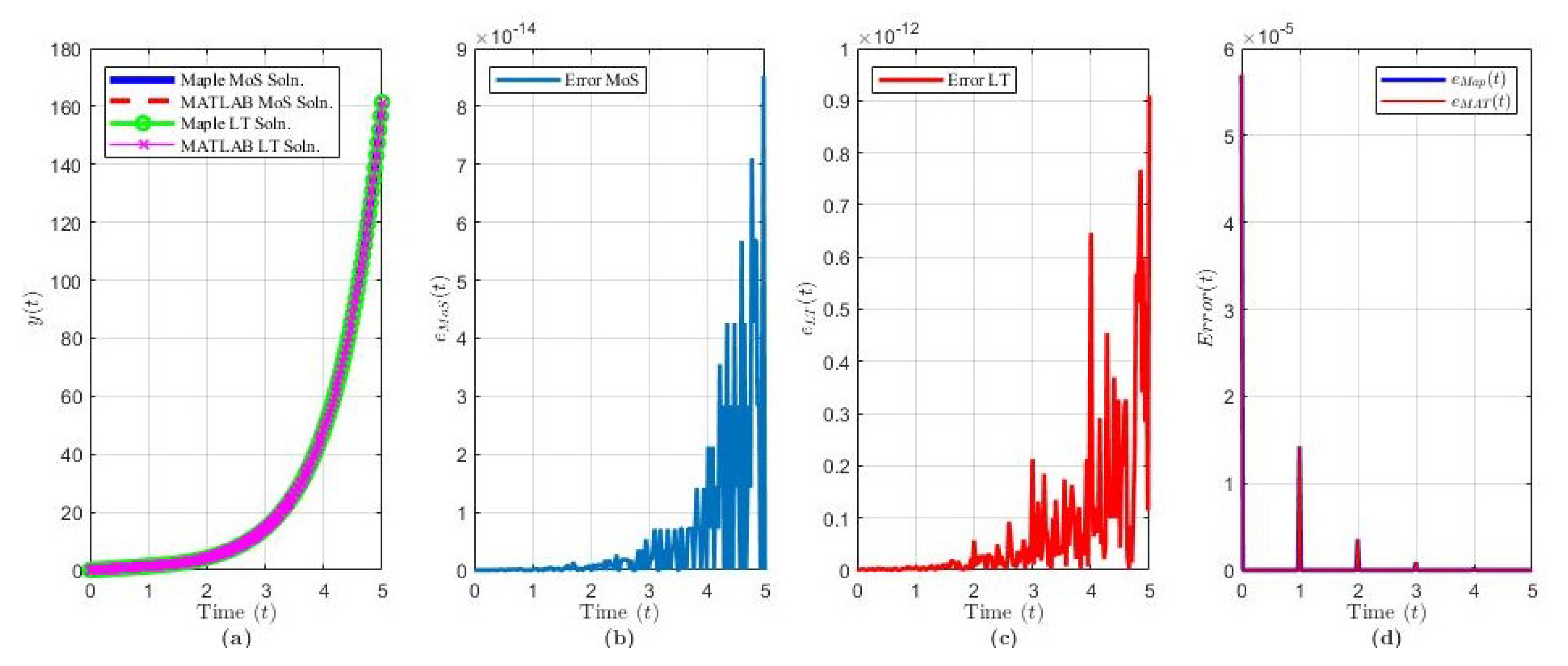
Example 3. Considerwhere , , and . This example was utilized in [36] to evaluate the performance of a numerical method for solving linear NDDEs using the generalized Lambert W function [55,56]. Applying MoS for a few partitions, we obtained the following analytical solution: Taking the LT of Equation (21), we obtained the quasi-polynomial , which has a real pole at with residue (from Equation (4)). The remaining poles and residues are given by the sequence for and , respectively. For large , these poles approach for (see [14]). Since , then, from the stability analysis, the solution will be unstable. Applying the ILT and Cauchy’s residue theorem, we obtained the LT solution of : The solution of Example 3 via MoS (over
intervals) and LT (
) and in each software program is shown in
Figure 4a.
Figure 4b,c shows that, as
, the variance between each software increases exponentially.
Figure 4d indicates that the accuracy of the LT solution improves exponentially as
t increases for both programs, and with noticeable spikes every
. Compared to the non-neutral examples, NDDE solutions have a higher complexity and, thus, one software may be more beneficial to use vs. another.
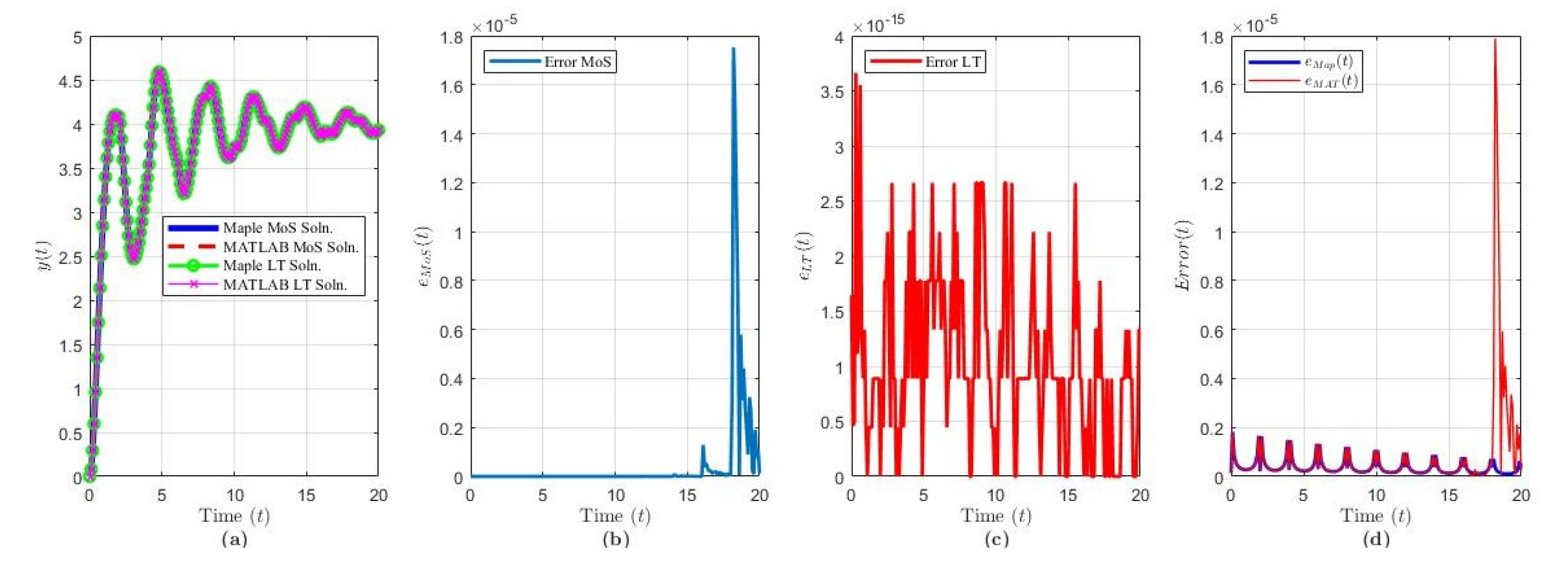
Example 4. Considerwhere , , and . This second example was first presented in [57] to study the superconvergence of continuous Galerkin finite element methods for linear NDDEs. Applying the MoS, the following analytical solution of over the interval was obtained, where m is the number of intervals: The characteristic equation of the system is given by , which has a real pole at with residue . The remaining poles and residues are given by the sequence for and , respectively. These poles are exactly given by for (see [14]). Since and Re, then, from the stability analysis, the solution will be stable. Applying the ILT and Cauchy’s residue theorem, we obtained the LT solution of : The solution of Example 4 via MoS (over
intervals) and LT (
) and in each software program is shown in
Figure 5a.
Figure 5b,c shows that the variance between each software is of order
and, as
, the error decreases with peak errors every
for
.
Figure 5d indicates that the accuracy of the LT solution improves as
t increases for both programs, and has an interesting spike located around
.
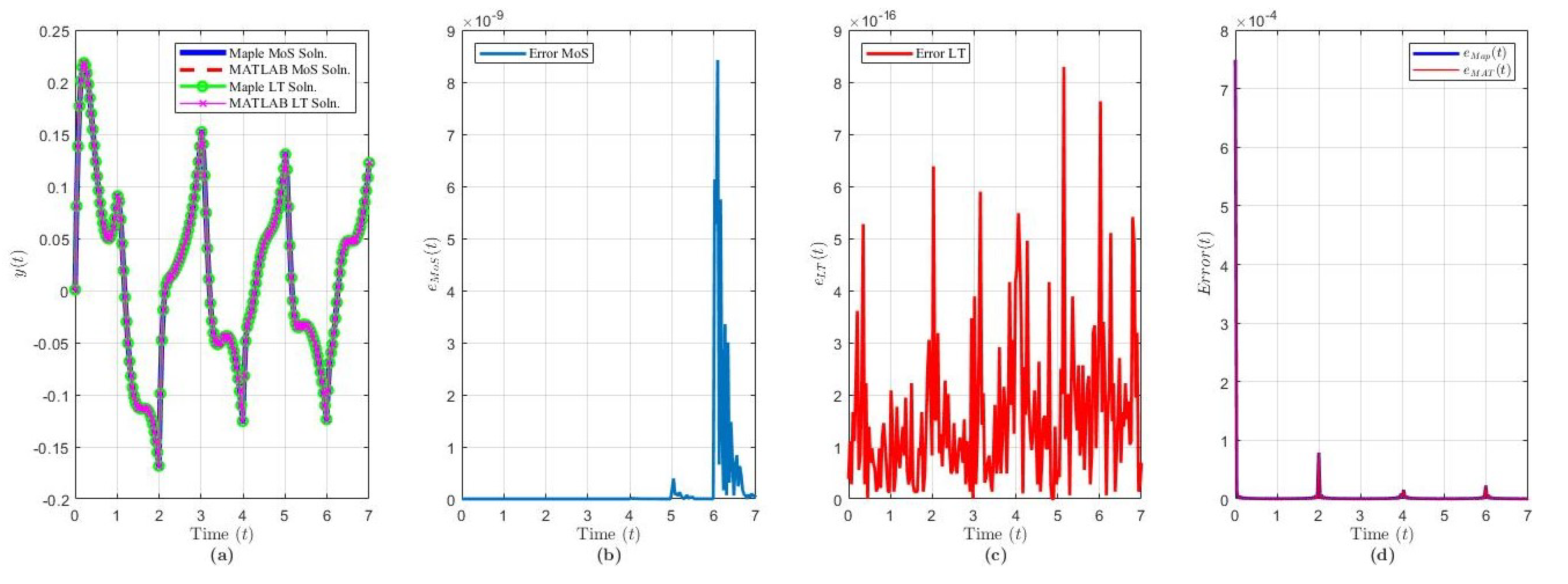
Example 5. Let us considerwhere and . The third example does not contain a state-dependent delay term. This equation is governed by the characteristic quasi-polynomial given by , which has a real pole at with residue . The other poles are given by the sequence . For large , these poles approach for (see [14]). The corresponding residues are given by . Applying the ILT and Cauchy’s residue theorem, we obtained the LT solution of : The solution of Example 5 via MoS (over
intervals) and LT (
) and in each software program is shown in
Figure 6a.
Figure 6b,c shows that the variance between each software is of order
via MoS and order
via LT. From
Figure 6d, as
, the error decreases with peak errors every
for
. This indicates that the accuracy of the LT solution improves as
t increases for both programs, and has an interesting spike located around
.
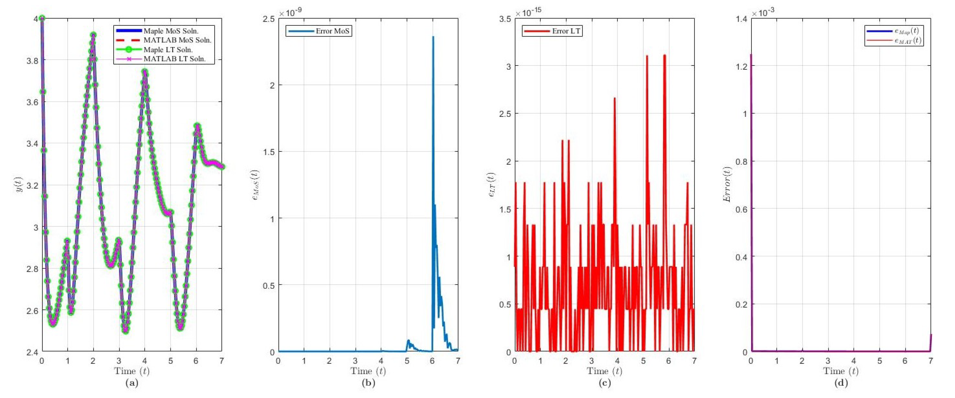
Example 6. Let us considerwhere , , and . The fourth example has the characteristic quasi-polynomial given by , which has no real poles. The complex poles are given by the sequence . For large , these poles approach for (see [14]). The corresponding residues are given by . Applying the ILT and Cauchy’s residue theorem, we obtained the LT solution of : The solution of Example 6 via MoS (over
intervals) and LT (
) and in each software program is shown in
Figure 7a.
Figure 7b,c shows that the variance between each software is of order
via MoS and order
via LT. We see similar deviances in the MoS solutions compared to Example 5 between each software. A larger timespan would be needed to deduce conclusions on the similarities of the LT solution between each software. From
Figure 6d, as
, the error decreases, with peak errors every
for
.
Example 7. Let us considerwhere , , and . The fifth example in Equation (25) has the characteristic quasi-polynomial given by , which has a real pole at with residue . The remaining poles are divided into two sequences (see [14]). One sequence of poles, , lies relatively close to the imaginary axis, which, for large , approaches for . The second sequence of poles, , is offset from the imaginary axis, which, for large , approaches for . The corresponding residues are given by . Then, the solution is of the form The solution of Example 7 via MoS (over
intervals) and LT (
) and in each software program is shown in
Figure 8a.
Figure 8b,c shows that the variance between each software is of order
via MoS and order
via LT. We see similar deviances in the MoS solutions near the boundary intervals compared to Example 5. Relative to previous NDDE examples, Example 7 has a larger error in the LT solution vs. the analytical MoS via both software, with an order of magnitude
as shown in
Figure 8d, despite the simplicity of the history function. Nevertheless, we can observe that, as
, the error decreases.
The computation times via each method and software are shown in
Table 2. We make the following notes regarding the time computation results:
From Maple MoS solutions, the order of time computation is as follows:
Example 5 > Example 6 > Example 7 > Example 4 > Example 3.
From Maple LT solutions, the order of time computation is as follows:
Example 7 > Example 3 > Example 6 > Example 5 > Example 4.
From MATLAB MoS solutions, the order of time computation is as follows:
Example 4 > Example 5 > Example 7 > Example 6 > Example 3.
From MATLAB LT solutions, the order of time computation is as follows:
Example 3 > Example 7 > Example 6 > Example 4 > Example 5.
From these results, we notice that the computation time is dependent on the complexity of the history function, the number of terms used in the LT solution, the number of intervals used in the MoS solution, and the magnitude of the parameters of the NDDE. Regarding MoS solutions, Examples 4 and 5 both have a complicated history function (one is a fourth-order polynomial and the other is periodic), and we observe that both programs took longer to compute the solutions. Regarding LT solutions, Examples 3 and 7 took the most time to compute via both software, even though Example 1 had the most terms. The differences between these examples is that Example 7 consisted of an extra sequence of poles due to the different delays in the state-dependent term and the derivative-of-state-dependent term. Nevertheless, Example 3 was found to be the quickest to compute via MoS for both softwares, whereas Examples 4 and 5 were found to be the quickest to compute via LT. We also note that, in all cases, Maple’s computation time was found to significantly outrank MATLAB’s computation time.
We notice that Examples 3 and 4 exhibit similar times since we used the same solution structure in both programs, compatible functions between programs, number of terms to be computed, and number of intervals to integrate over. Given the number of terms to be computed for the LT solution, the computation time was higher for both programs compared to the MoS solutions. However, with the use of MATLAB’s symbolic toolbox functions, the computation time for the LT solution was reduced by 4x compared to Maple for both examples.
5. Conclusions
In this paper, we investigated the symbolic mathematical computational performance of the software program Maple and the programming language MATLAB when applying the method of steps (MoS) and the Laplace transform (LT) methods to solve neutral and retarded linear DDEs. Of particular interest was comparing how these programs performed. The exact, analytic MoS solution was used to aid in this comparison. However, the main reason for why most of the graphs only include the first 5–10 time-intervals is due to the fact that the method of steps often could not compute the solution beyond these intervals. The Laplace solution is an infinite series, which requires one to compute the relevant poles along with their associated residues. We computed the analytical solutions using Maple and MATLAB in order to take advantage of their respective symbolic computation features. The accuracy of the Laplace method solutions were measured by comparing them with those obtained by the method of steps. The Laplace method produces an analytical solution that can be evaluated at any particular value of time. The results obtained emphasize that symbolic computational software is a powerful tool, capable of computing analytic solutions for linear delay differential equations, including neutral ones. From a computational viewpoint, we found that the computation time is dependent on the complexity of the history function, the number of terms used in the LT solution, the number of intervals used in the MoS solution, and the DDE parameters. We found that, for linear non-neutral DDEs, MATLAB symbolic computations were faster than the ones from Maple. However, for the linear neutral DDEs, which are often more difficult to solve, Maple was faster. Regarding accuracy, it is important to point out that we compared Maple and MATLAB via MoS and LT. The differences between both software were smaller for the LT in comparison to the MoS. In addition, the accuracy of the LT solutions using Maple were, in a few cases, slightly better than the ones generated by MATLAB. However, both were reliable, but we can mention that Maple lightly surpasses MATLAB in symbolic computation due to its symbolic capabilities/nature. Finally, we would like to mention some limitations of the LT irrespective of the software choice. The LT method is only applicable for linear DDEs due to the Laplace transform definition. Thus, nonlinear DDEs should be solved by other means. In addition, we implemented the LT for scalar linear DDEs with constant coefficients and a finite number of delays. However, the LT method can also be extended to solve first-order linear DDE systems. In this work, we applied the LT method to homogeneous and non-homogenous DDEs. Future works that are in progress include solving linear non-homogeneous DDEs with Dirac delta function inputs, with one related goal being to develop a Green’s function type kernel.


