Article

Optimal Control of an HIV Model with Gene Therapy and Latency Reversing Agents

Department of Mathematics, Winthrop University, 701 Oakland Ave., Rock Hill, SC 29733, USA
*
Author to whom correspondence should be addressed.
Math. Comput. Appl. 2021, 26(4), 77; https://doi.org/10.3390/mca26040077
Submission received: 29 September 2021 / Revised: 4 November 2021 / Accepted: 9 November 2021 / Published: 12 November 2021
(This article belongs to the Section Natural Sciences)

Abstract

:
In this paper, we study the dynamics of HIV under gene therapy and latency reversing agents. While previous works modeled either the use of gene therapy or latency reversing agents, we consider the effects of a combination treatment strategy. For constant treatment controls, we establish global stability of the disease-free equilibrium and endemic equilibrium based on the value of R 0 . We then consider time-dependent controls and formulate an associated optimal control problem that emphasizes reduction of the latent reservoir. Characterizations for the optimal control profiles are found using Pontryagin’s Maximum Principle. We perform numerical simulations of the optimal control model using the fourth-order Runge–Kutta forward-backward sweep method. We find that a combination treatment of gene therapy with latency reversing agents provides better remission times than gene therapy alone. We conclude with a discussion of our findings and future work.

1. Introduction

Uncovering a functional cure or new preventative methods for the Human Immunodeficiency Virus (HIV) remains a challenge and focus of medical research. Acquiring HIV infection leads to a weakened immune system that leaves the host more susceptible to other infections and diseases. If HIV goes untreated for a prolonged interval of time, the infection can progress to acquired immunodeficiency syndrome (AIDS).
Antiretroviral therapy (ART) remains the primary method of limiting the spread of the virus. Though ART is effective at reducing the viral load to undetectable levels, even short lapses in treatment grant the virus the capability to rapidly rebound within weeks [1]. This can be attributed to the presence of a minute number of latently infected cells that store the genetic information of HIV yet are not actively replicating virions, thus evading typical ART strategies. If an individual stops taking ART for a period of time, natural reactivation of this latent reservoir can quickly lead to an increase in viral load. In the search for a functional cure that would alleviate the need for lifelong ART medication, recent studies suggested the usage of other methods such as gene therapy and latency reversing agents to help overcome the limitations of ART treatments [1].
A motivating example for the usage of gene therapy is the Berlin Patient, an individual who received an allogeneic transplant from a donor in hopes of curing his leukemia. This transplant introduced C C R 5 -deficient bone marrow [1,2]. The CCR5 receptor is the main coreceptor in which HIV attaches itself to the target cell, and thus the introduction of this bone marrow transplant into the patient’s body reduced the number of susceptible target CD4 + T-cells by replacing the CCR5 + cells with the more resilient CCR5 cells [3]. In the subsequent 10 years following the procedure, a rebound of the virus in the Berlin Patient was not observed [1].
The CRISPR-Cas9 gene therapy program seeks to provide a similar treatment to the bone marrow transplant that the Berlin Patient received by altering the DNA of the susceptible target CD4 + T-cells to negatively express the CCR5 coreceptor [4]. However, current levels of efficacy are insufficient to provide a reasonable level of reduction in viral load, and thus, combinations of strategies will likely be needed to increase the odds of reaching a functional cure [1]. To supplement the efficacy of current gene therapy, as well as to explicitly address the existence of the latent reservoir, we additionally consider latency-reversing agents (LRAs), also generally referred to as “shock and kill” therapy. LRAs activate latently infected cells so they can be detected and attacked by the immune system or by ART [5,6].
Mathematical models provide a useful framework for exploring disease dynamics and associated treatment programs [7]. Over the past several decades, systems of ordinary differential equations were used to better understand the complex interaction of HIV and the immune system, as well as explore potential treatment options in the search for a functional cure [8,9,10,11,12]. Additionally, recent HIV modeling approaches incorporated latent reservoirs to better understand viral rebounds [13,14,15,16,17]. In 2018, Ke et al. explored the dynamics of LRAs through a mathematical model with three compartments: latently infected cells, cells activated by LRA treatment, and refractory cells temporarily resistant to LRA treatment [6]. In 2019, Davenport et al. proposed a mathematical model for the use of gene therapy in HIV prevention [1]. The model describes the dynamics between a susceptible population and refractory (nonsusceptible) population that has received gene therapy, in addition to standard interactions with actively infected cells and free virions. The authors used the model to establish efficacy thresholds for gene therapy to achieve a functional cure for HIV for various ranges of basic reproductive ratios, and noted that combination strategies may serve to reduce the efficacy needed from any individual treatment.
The goal of this paper is to build upon the works of Ke et al. [6] and Davenport et al. [1] by constructing and analyzing a mathematical model that incorporates the combination of gene therapy and LRA treatment. We aim to explore possible synergies between these treatment methods for both constant and time-dependent descriptions of the treatment controls.

2. Model Development

In this paper, we use the following system of differential equations to model the dynamics of an HIV infection under the combined effects of CRISPR-Cas9 gene therapy, latency reversing agents, and antiretroviral therapy. For the purpose of our work, we are interested in the interactions between CCR5 cells T u , CCR5 + cells T s , latently infected cells L, actively infected cells I, and free virions V.
d T u d t = λ f δ T T u d T s d t = λ ( 1 f ) δ T T s β T s V d L d t = ϵ β T s V ( α + η + δ ) L + γ I d I d t = ( 1 ϵ ) β T s V + ( α + η ) L ( c + δ + γ ) I d V d t = p I δ V V
In system (1), f represents the fraction of CD4 + T-cells that become nonsusceptible to HIV as a result of gene therapy. Susceptible T s cells become latently infected at an interaction rate of ϵ β and actively infected at an interaction rate of ( 1 ϵ ) β . Latently infected cells are naturally activated at a rate of η . Latency reversing agents are activated cells at a rate of α and cells stay activated for a duration of 1 γ days before returning to the latent stage. Actively infected cells are removed through antiretroviral therapy at a rate of c, and produce free virions at a rate of p. The target cell death rate, infected cell death rate, and virus clearance rate are given by δ T , δ , and δ V , respectively. We summarize these parameter roles, along with baseline values gathered from literature, in Table 1.

3. Model Analysis

Assuming system (1) is subject to non-negative initial conditions, we note that the system is invariant in the non-negative orthant. Additionally, because the associated vector field is continuously differentiable, given a set of initial conditions there exists a unique solution to our system by the Picard–Lindelof Theorem [20].
Let N denote the total cell population so that N ( t ) = T u ( t ) + T s ( t ) + L ( t ) + I ( t ) and Δ = min { δ T , δ } . Then lim sup t N ( t ) λ Δ . This also implies that lim sup t V ( t ) p λ Δ δ V . Thus, solution trajectories of system (1) remain bounded over time.

3.1. Basic Reproductive Ratio: R 0

We denote the disease-free equilibrium by E 0 = T u 0 , T s 0 , 0 , 0 , 0 = λ f δ T , λ ( 1 f ) δ T , 0 , 0 , 0 and calculate R 0 using the next generation matrix. To derive the next generation matrix, we first calculate the transmission matrix F and the transition matrix V evaluated at E 0 . These are given by:
F = 0 0 0 0 0 0 0 0 0 β λ ( 1 f ) δ T 0 0 0 0 ϵ β λ ( 1 f ) δ T 0 0 0 0 ( 1 ϵ ) β λ ( 1 f ) δ T 0 0 0 0 0
and
V = δ T 0 0 0 0 0 δ T 0 0 0 0 0 α + η + δ γ 0 0 0 ( α + η ) c + δ + γ 0 0 0 0 p δ V .
R 0 is the spectral radius of the next generation matrix F V 1 , thus
R 0 = β λ p ( 1 f ) ( α + η + δ ( 1 ϵ ) ) δ T δ V ( ( α + η + δ ) ( c + δ ) + δ γ ) .

3.2. Global Stability of the Disease Free Equilibrium

Theorem 1.
When R 0 1 , the disease free equilibrium E 0 is globally asymptotically stable.
Proof. 
Consider the Lyapunov function
L = T u T u 0 T u 0 ln T u T u 0 + T s T s 0 T s 0 ln T s T s 0 + α + η α + η + ( 1 ϵ ) δ L + α + δ + η α + η + ( 1 ϵ ) δ I + β λ ( 1 f ) δ T δ V V .
Then
d L d t = 1 T u 0 T u ( λ f δ T T u ) + 1 T s 0 T s ( λ ( 1 f ) δ T T s β T s V ) + α + η α + η + ( 1 ϵ ) δ ( ϵ β T s V ( δ + η + α ) L + γ I ) + α + δ + η α + η + ( 1 ϵ ) δ ( ( 1 ϵ ) β T s V + ( η + α ) L ( δ + c + γ ) I ) + β λ ( 1 f ) δ T δ V ( p I δ V V ) = λ f 2 T u T u 0 T u 0 T u + λ ( 1 f ) 2 T s T s 0 T s 0 T s + ( α + η ) γ α + η + ( 1 ϵ ) δ + β λ p ( 1 f ) δ T δ V ( α + δ + η ) ( δ + c + γ ) α + η + ( 1 ϵ ) δ I = λ f 2 T u T u 0 T u 0 T u + λ ( 1 f ) 2 T s T s 0 T s 0 T s + ( δ + c ) ( ( α + δ + η ) + δ γ ) α + η + ( 1 ϵ ) δ ( R 0 1 ) I .
Since the arithmetical mean is always greater than or equal to the geometric mean, it follows that R 0 1 implies d L d t 0 for all T u , T s , L , I , V R 0 . Hence, it is a consequence of LaSalle’s Invariance Theorem [20] that the disease free equilibrium is globally asymptotically stable. □

3.3. Global Stability of the Endemic Equilibrium

Theorem 2.
When R 0 > 1 , there exists a unique endemic equilibrium ( T u * , T s * , L * , I * , V * ) .
Proof. 
To establish equilibria of system (1), we must solve the following system of equations:
0 = λ f δ T T u *
0 = λ ( 1 f ) δ T T s * β T s * V *
0 = ϵ β T s * V * ( α + η + δ ) L * + γ I *
0 = ( 1 ϵ ) β T s * V * + ( α + η ) L * ( c + δ + γ ) I *
0 = p I * δ V V *
We see from Equation (2) that T u * = λ f δ T . If I * = 0 , we recover our disease free equilibrium λ f δ T , λ ( 1 f ) δ T , 0 , 0 , 0 . To solve for an endemic equilibrium, suppose I * 0 and use Equations (3), (4), and (6) to solve for T s * , L * and V * in terms of I * :
T s * = λ ( 1 f ) δ T + β V * L * = ϵ β T s * V * + γ I * α + η + δ V * = p I * δ V .
Substituting these expressions into Equation (5), we see that the number of internal equilibria is determined by the number of solutions to f ( I * ) = 0 , where
f ( I * ) = ( c + γ + δ ) + ( 1 f ) p β ( 1 ϵ ) λ δ T δ V + p β I * + ( α + η ) ( γ δ T δ V + p β ( γ I * + ( 1 f ) ϵ λ ) ( α + δ + η ) ( δ T δ V + p β I * ) .
Note that
  • f ( 0 ) = ( c + δ ) ( α + δ + η ) + δ γ α + δ + η ( R 0 1 ) ;
  • f ( I * ) = ( 1 f ) p 2 β 2 λ ( α + ( 1 ϵ ) δ + η ) ( α + δ + η ) ( p β I * + δ T δ V ) 2 ; and
  • lim I * f ( I * ) = c δ ( α + γ + δ + η ) α + δ + η .
Thus, when R 0 > 1 , f ( I * ) has a unique positive root. It follows that there exists a unique endemic equilibrium when R 0 > 1 .
Theorem 3.
When R 0 > 1 , the endemic equilibrium is globally asymptotically stable.
Proof. 
Notate the endemic equilibrium as ( T u * , T s * , L * , I * , V * ) and consider the Lyapunov function
L = T u T u * T u * ln T u T u * + T s T s * T s * ln T s T s * + α + η α + η + ( 1 ϵ ) δ L L * L * ln L L * + α + η + δ α + η + ( 1 ϵ ) δ I I * I * ln I I * + β T s * δ V V V * V * ln V V * .
Then
d L d t = 1 T u * T u ( λ f δ T T u ) + 1 T s * T s ( λ ( 1 f ) δ T T s β T s V ) + α + η α + η + ( 1 ϵ ) δ 1 L * L ( ϵ β T s V ( δ + η + α ) L + γ I ) + α + δ + η α + η + ( 1 ϵ ) δ 1 I * I ( ( 1 ϵ ) β T s V + ( η + α ) L ( δ + c + γ ) I ) + β T s * δ V 1 V * V ( p I δ V V ) = λ f 2 T u T u * T u * T u + δ T T s * 2 T s T s * T s * T s + 2 β T s * V * β T s * V * T s * T s β T s * V * I V * I * V + ( α + η ) ϵ β T s * V * α + η + ( 1 ϵ ) δ 1 L * T s V L T s * V * + ( α + η ) γ I * α + η + ( 1 ϵ ) δ 1 I L * I * L + ( α + δ + η ) ( 1 ϵ ) β T s * V * α + η + ( 1 ϵ ) δ 1 I * T s V I T s * V * + ( α + δ + η ) ( α + η ) L * α + η + ( 1 ϵ ) δ 1 I * L I L * .
Since
β T s * V * = ( α + η ) ϵ β T s * V * α + η + ( 1 ϵ ) δ + ( α + δ + η ) ( 1 ϵ ) β T s * V * α + η + ( 1 ϵ ) δ
we have
d L d t = λ f 2 T u T u * T u * T u + δ T T s * 2 T s T s * T s * T s + ( α + η ) γ I * α + η + ( 1 ϵ ) δ 2 I L * I * L I * L I L * + ( α + η ) ϵ β T s * V * α + η + ( 1 ϵ ) δ 4 L * T s V L T s * V * I * L I L * T s * T s I V * I * V + ( α + δ + η ) ( 1 ϵ ) β T s * V * α + η + ( 1 ϵ ) δ 3 I * T s V I T s * V * T s * T s I V * I * V .
Thus, d L / d t < 0 for all ( T u , T s , L , I , V ) R 0 5 , ( T u , T s , L , I , V ) ( T u * , T s * , L * , I * , V * ) , and so the endemic equilibrium is globally asymptotically stable when R 0 > 1 .

4. Model Predictions

Using the parameter values found in Table 1, in the absence of any treatment we find that system (1) has a baseline basic reproductive ratio of R 0 = 8.6948 . This aligns with typical HIV basal reproductive ratios as described in [1]. By allowing f to vary, we find that R 0 ( f ) < 1 when f > 0.8850 , i.e., gene therapy alone is capable of achieving a functional cure provided that at least 88.50% of susceptible target cells become refractory in response to gene therapy treatment. For a combination treatment strategy, we find that using upper limits for the LRA activation rate of α = 1.8 and ART removal rate of c = 1 reduces the effectiveness of gene therapy required to achieve R 0 ( f ) < 1 to f > 0.8150 .
However, given current optimistic gene therapy efficacy rates of f = 0.3 [1], we may consider instead the potential benefits of using gene therapy in combination with LRAs and ART therapy to achieve an elongated remission time. We assume the reactivation rate r of cells from the latently infected reservoir is directly proportional to the steady-state size of the latent reservoir L * , i.e., r = η L * , where η is the natural activation rate of a latently infected cell. Using gene therapy alone at current efficacy levels of f = 0.3 , we find that the duration of remission 1 / r is 10.49 days. However, using an LRA activation rate of α = 1.8 and ART removal rate of c = 1 
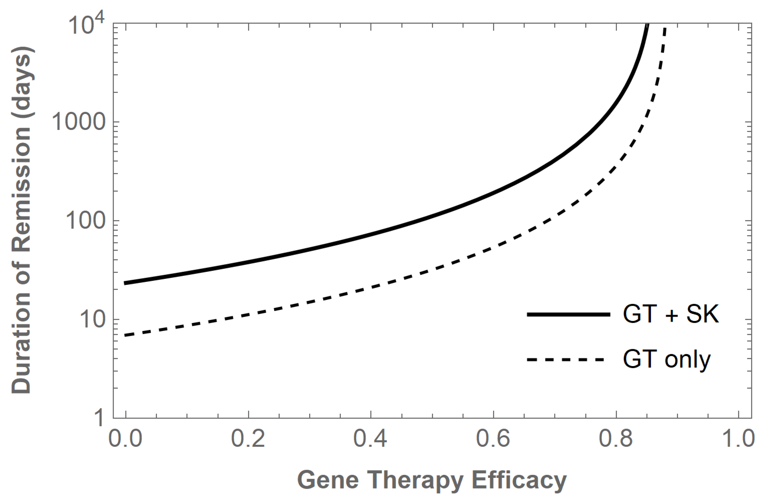
improves the duration of remission to 88.13 days. We summarize the added benefit of LRA+ART shock and kill treatment for other levels of gene therapy efficacy in Figure 1.
These results demonstrate that both gene therapy and shock and kill treatments can contribute to extending remission times and progressing toward a functional cure. To better understand optimal treatment protocols and allow for nonconstant treatment controls, we turn to an optimal control model in the sections to follow.

5. Optimal Control

Applying constant controls for arbitrarily long periods of time may be unsustainable, thus we next aim to find an optimal treatment strategy over a finite time horizon that minimizes the total burden of infection while also minimizing the cost of implementing such a strategy. We introduce into the model time-dependent controls for f ( t ) , the gene therapy treatment, α ( t ) , the latent reservoir activation, and c ( t ) , the ART treatment. This yields the system
d T u d t = λ f ( t ) δ T T u d T s d t = λ ( 1 f ( t ) ) δ T T s β T s V d L d t = ϵ β T s V ( α ( t ) + η + δ ) L + γ I d I d t = ( 1 ϵ ) β T s V + ( α ( t ) + η ) L ( c ( t ) + δ + γ ) I d V d t = p I δ V V
The objective functional we choose to minimize is given by
J ( f , α , c ) = 0 τ A 1 L + A 2 I + A 3 V + A 4 f 2 + A 5 α 2 + A 6 c 2 d t ,
where A 1 , A 2 , A 3 , A 4 , A 5 , and A 6 are positive weights and τ is the final time. The weights A 4 , A 5 , and A 6 are associated with quadratic costs of implementing the gene therapy, LRA, and ART treatments. The set of admissible control functions is given by
U = { ( f , α , c ) L ( 0 , τ ) 3 | ( f ( t ) , α ( t ) , c ( t ) ) [ 0 , 1 ] × [ 0 , α m a x ] × [ 0 , c m a x ] t [ 0 , τ ] } .
Thus, we seek an optimal control set ( f * , α * , c * ) such that
J ( f * , α * , c * ) = m i n { J ( f , α , c ) | ( f , α , c ) U } .
We proceed by utilizing Pontryagin’s Maximum Principle [21] to exchange the problem of minimizing the objective functional for a problem of finding the pointwise minimum of the following Hamiltonian with respect to f, α , and c:
H = A 1 L + A 2 I + A 3 V + A 4 f 2 + A 5 α 2 + A 6 c 2 + λ 1 ( λ f δ T T u ) + λ 2 ( λ ( 1 f ) δ T T s β T s V )
+ λ 3 ( ϵ β T s V L ( δ + η + α ) ) + λ 4 ( ( 1 ϵ ) β T s V + L ( η + α ) I ( γ + δ + c ) ) + λ 5 ( p I δ V V )
where λ 1 , λ 2 , λ 3 , λ 4 , and λ 5 are the adjoint or costate variables associated with the state variables T u , T s , L, I , and V. The following theorem establishes the existence of an optimal control set and characterizations for the optimal control functions.
Theorem 4.
There exists an optimal control set ( f * , α * , c * ) that minimizes J ( f , α , c ) over U. Furthermore, there exist adjoint variables λ 1 , λ 2 , λ 3 , λ 4 , and λ 5 that satisfy the following system of differential equations:
d λ 1 d t = H T u = δ T λ 1 d λ 2 d t = H T s = ( δ T + β V ) λ 2 ϵ β V λ 3 ( 1 ϵ ) β V λ 4 d λ 3 d t = H L = A 1 + ( δ + η + α ) λ 3 ( η + α ) λ 4 d λ 4 d t = H I = A 2 γ λ 3 + ( δ + γ + c ) λ 4 p λ 5 d λ 5 d t = H V = A 3 + β T S λ 2 ϵ β T S λ 3 ( 1 ϵ ) β T S λ 4 + δ V λ 5
with transversality conditions λ 1 ( τ ) = λ 2 ( τ ) = λ 3 ( τ ) = λ 4 ( τ ) = λ 5 ( τ ) = 0 . Also, the optimal control set has the characterization:
f * = m i n 1 , m a x 0 , λ ( λ 2 λ 1 ) 2 A 4
α * = m i n α m a x , m a x 0 , L λ 3 + I λ 4 2 A 6
c * = m i n c m a x , m a x 0 , I λ 4 2 A 5
Proof. 
Using Corollary 4.1 of [22], the existence of an optimal control set follows from the Lipschitz property of system (1) with respect to the state variables, a priori boundedness of the state solutions established in Section 3, and the convexity of the integrand of J with respect to ( f , α , c ) .
By applying Pontryagin’s Maximum Principle, the adjoint variables must satisfy system (8) with zero final time conditions. To obtain the characterizations of the optimal controls, we solve H f = H α = H c = 0 on the interior of the control set U. Using the bounds on the controls, we obtain the desired characterization. □
We note that the optimality system consists of the state system (7) with initial time conditions, the adjoint system (8) with final time conditions, and the above characterizations of the optimal controls. Due to the opposite time orientations of the state and adjoint systems, the uniqueness of the optimal control solution is only guaranteed for small final time τ [23].

6. Numerical Results

We follow the method presented in [24] and utilize an iterative procedure to numerically solve the boundary value problem associated with the above optimality system. Using an initial guess for each of the three controls, we first solve the state system forward in time using a fourth-order Runge–Kutta procedure. Using the resulting state values and final time values, we next solve the adjoint system with transversality conditions backwards in time, again with a fourth-order Runge–Kutta scheme. The controls are then updated using a convex combination of the previous control values and the values resulting from the characterizations of each control. This iterative process then repeats until convergence, which occurs when the maximum relative error between each of the state variables, adjoint variables, and controls over successive iterations is less than a specified value δ .
The optimality system was solved using parameter values found in Table 1, a final time of t f = 10 days, and the following initial conditions: T u ( 0 ) = 0 , T S ( 0 ) = 10 6 , L ( 0 ) = 1 , I ( 0 ) = 10 4 , and V ( 0 ) = 10 6 . Furthermore, reasonable estimates for the weights A 1 , A 2 , A 3 , A 4 , A 5 , and A 6 are necessary to ensure convergence is achieved and to obtain meaningful optimal control profiles. Using the extra degree of freedom to select A 3 = 1 , we then solve A 1 L = A 2 I = A 3 V = A 4 0 t f f 2 d t = A 5 0 t f α 2 d t = A 6 0 t f c 2 d t to balance the contributions of each weight, where we substitute the median values of each state variable and control: L = 16 , 810.8 , I = 36 , 405.3 , V = 1 , 585 , 277 , f = 0.5 , α = 0.9 , c = 0.5 . We further adjust A 1 by a factor of 10 to prioritize reduction of the latent reservoir. This procedure yields weights of A 1 = 943.01 , A 2 = 43.54 , A 3 = 1 , A 4 = 634 , 111 , A 5 = 195 , 713 , A 6 = 634 , 111 .
The optimal control profiles f * , α * , and c * are shown in Figure 2.
We see in each case the maximum allowable control being applied through approximately day 5–6 before steadily decreasing. This allows for optimal reduction in the total burden of infection in the early days of the treatment regimen before the associated quadratic costs of treatment become too large. We note that including shock and kill treatment allows for the optimal efficacy of gene therapy to decline sooner. The impact of the optimal controls on HIV state variables may be seen in Figure 3. In the absence of any controls, the latent reservoir reaches a peak of 269,051 cells, while using gene therapy alone reduces this maximum burden to 229,443 cells. A combination strategy with both gene therapy and shock and kill therapy is far more effective, reducing the peak burden to 66,486 cells and quickly suppressing the latent reservoir to negligible levels. We observe similar results with the actively infected cell population, beginning with a peak of 639,879 cells with no treatment while achieving a reduced maximum burden of 392,943 cells using an optimal combination treatment strategy. The free virion particles are also reduced from a peak of 2.769 × 10 7 virions to 1.699 × 10 7 virions under optimal combination treatment. To summarize, the optimal combination of gene therapy and LRA/ART therapy yields an overall decrease in the peak latent, actively infected, and free virion population levels of 75.33 % , 38.59 % , and 38.63 % , respectively. As expected, the selection of weights above prioritized a larger reduction in the latent reservoir, which will be crucial for novel treatment strategies aiming to prolong remission times and progress towards a functional cure for HIV.

7. Conclusions

In this paper, we developed a mathematical model for HIV which includes the latent reservoir and captures the dynamics of combination treatment strategies using gene therapy, latency reversing agents, and antiretroviral therapy. We performed a complete global stability analysis of the model, calculating the basic reproductive ratio and establishing the existence and global stability of both disease free and endemic equilibria. We then computed threshold levels of treatment efficacy needed to achieve a functional cure, or alternatively, prolong remission times when reaching the disease-free equilibrium, which would require prohibitively high levels of treatment effectiveness. During this analysis, we showcased and quantified the added benefits of supporting gene therapy treatments with shock and kill methods designed to attack the latent reservoir.
Given that multiple treatment strategies provided tangible benefits to the long-term progression of HIV infection, we next formulated an optimal control problem to achieve the largest reduction in infected compartments using nonconstant treatment profiles. Our results yielded a substantial reduction in the latent reservoir when using the optimal combination of gene therapy, latency reversing agents, and antiretroviral medication.
The model presented here has some limitations which can inspire future directions of study. We do not capture the diminished efficacy of treatments over time due to acquired drug resistance or virus mutation. The mass action description of the interaction between susceptible cells and free virions could also be refined to consider other limited infection rates. Furthermore, additional data should be collected to establish more reliable parameters and weights for the optimal control system. This will potentially allow for extended time windows in the numerical simulation and improve the discovery of optimal combination treatment regimens.

Author Contributions

Conceptualization, Z.A., K.A., A.G. and P.H.; methodology, Z.A., K.A., A.G. and P.H.; formal analysis, Z.A., K.A., A.G. and P.H.; visualization, Z.A., K.A., A.G. and P.H.; writing—original draft preparation, Z.A., K.A., A.G. and P.H.; writing—review and editing, Z.A. and K.A.; funding acquisition, Z.A. and K.A. All authors have read and agreed to the published version of the manuscript.

Funding

This research was funded by South Carolina IDeA Networks for Biomedical Research Excellence (grant number P20GM103499-20) through the National Institute of General Medical Sciences, National Institutes of Health.

Acknowledgments

This work was supported by grant P20GM103499-20 (SC INBRE) from the National Institute of General Medical Sciences, National Institutes of Health. The authors additionally wish to thank the two reviewers for their insightful feedback which improved the quality of this manuscript.

Conflicts of Interest

The authors declare no conflict of interest.

References

  1. Davenport, M.P.; Khoury, D.S.; Cromer, D.; Lewin, S.R.; Kelleher, A.D.; Kent, S.J. Functional cure of HIV: The scale of the challenge. Nat. Rev. Immunol. 2019, 19, 45–54. [Google Scholar] [CrossRef] [PubMed]
  2. Hütter, G.; Bodor, J.; Ledger, S.; Boyd, M.; Millington, M.; Tsie, M.; Symonds, G. CCR5 targeted cell therapy for HIV and prevention of viral escape. Viruses 2015, 7, 4186–4203. [Google Scholar] [CrossRef] [PubMed] [Green Version]
  3. Tebas, P.; Stein, D.; Tang, W.W.; Frank, I.; Wang, S.Q.; Lee, G.; Spratt, S.K.; Surosky, R.T.; Giedlin, M.A.; Nichol, G.; et al. Gene Editing of CCR5 in Autologous CD4 T Cells of Persons Infected with HIV. N. Engl. J. Med. 2014, 370, 901–910. [Google Scholar] [CrossRef] [PubMed] [Green Version]
  4. Kaminski, R.; Chen, Y.; Fischer, T.; Tedaldi, E.; Napoli, A.; Zhang, Y.; Karn, J.; Hu, W.; Khalili, K. Elimination of HIV-1 genomes from human T-lymphoid cells by CRISPR/Cas9 gene editing. Sci. Rep. 2016, 6, 1–15. [Google Scholar]
  5. Hill, A.L.; Rosenbloom, D.I.; Fu, F.; Nowak, M.A.; Siliciano, R.F. Predicting the outcomes of treatment to eradicate the latent reservoir for HIV-1. Proc. Natl. Acad. Sci. USA 2014, 111, 13475–13480. [Google Scholar] [CrossRef] [PubMed] [Green Version]
  6. Ke, R.; Conway, J.M.; Margolis, D.M.; Perelson, A.S. Determinants of the efficacy of HIV latency-reversing agents and implications for drug and treatment design. JCI Insight 2018, 3, e123052. [Google Scholar] [CrossRef] [PubMed]
  7. Nowak, M.; May, R.M. Virus Dynamics: Mathematical Principles of Immunology and Virology; Oxford University Press: Oxford, UK, 2000. [Google Scholar]
  8. Ogunlaran, O.M.; Oukouomi Noutchie, S.C. Mathematical model for an effective management of HIV infection. BioMed Res. Int. 2016, 2016, 4217548. [Google Scholar] [CrossRef] [PubMed]
  9. Ribeiro, R.M.; Perelson, A.S. The analysis of HIV dynamics using mathematical models. In AIDS and Other Manifestations of HIV Infection, 4th ed.; Wormser, G.P., Ed.; Elsevier: New York, NY, USA, 2004; Chapter 35. [Google Scholar]
  10. Wodarz, D.; Nowak, M.A. Mathematical models of HIV pathogenesis and treatment. BioEssays 2002, 24, 1178–1187. [Google Scholar] [CrossRef] [PubMed]
  11. Duffin, R.P.; Tullis, R.H. Mathematical models of the complete course of HIV infection and AIDS. J. Theor. Med. 2002, 4, 215–221. [Google Scholar] [CrossRef] [Green Version]
  12. Rong, L.; Perelson, A.S. Modeling HIV persistence, the latent reservoir, and viral blips. J. Theor. Biol. 2009, 260, 308–331. [Google Scholar] [CrossRef] [PubMed] [Green Version]
  13. Wang, S.; Rong, L. Stochastic population switch may explain the latent reservoir stability and intermittent viral blips in HIV patients on suppressive therapy. J. Theor. Biol. 2014, 360, 137–148. [Google Scholar] [CrossRef] [PubMed]
  14. Vaidya, N.K.; Rong, L. Modeling pharmacodynamics on HIV latent infection: Choice of drugs is key to successful cure via early therapy. SIAM J. Appl. Math. 2017, 77, 1781–1804. [Google Scholar] [CrossRef] [Green Version]
  15. Cromer, D.; Pinkevych, M.; Rasmussen, T.A.; Lewin, S.R.; Kent, S.J.; Davenport, M.P. Modeling of antilatency treatment in HIV: What is the optimal duration of antiretroviral therapy-free HIV remission? J. Virol. 2017, 91, e01395-17. [Google Scholar] [CrossRef] [PubMed] [Green Version]
  16. Hill, A.L. Mathematical models of HIV latency. In HIV-1 Latency; Springer: Cham, Switzerland, 2017; pp. 131–156. [Google Scholar]
  17. Yan, C.; Wang, W. Modeling HIV dynamics under combination therapy with inducers and antibodies. Bull. Math. Biol. 2019, 81, 2625–2648. [Google Scholar] [CrossRef] [PubMed]
  18. Reeves, D.B.; Duke, E.R.; Hughes, S.M.; Prlic, M.; Hladik, F.; Schiffer, J.T. Anti-proliferative therapy for HIV cure: A compound interest approach. Sci. Rep. 2017, 7, 1–10. [Google Scholar] [CrossRef] [PubMed] [Green Version]
  19. Rong, L.; Perelson, A.S. Modeling latently infected cell activation: Viral and latent reservoir persistence, and viral blips in HIV-infected patients on potent therapy. PLoS Comput. Biol. 2009, 5, e1000533. [Google Scholar] [CrossRef] [PubMed] [Green Version]
  20. Kelley, W.G.; Peterson, A.C. The Theory of Differential Equations: Classical and Qualitative; Springer Science & Business Media: Berlin/Heidelberg, Germany, 2010. [Google Scholar]
  21. Pontryagin, L.S. Mathematical Theory of Optimal Processes; Routledge: Oxfordshire, UK, 2018. [Google Scholar]
  22. Fleming, W.H.; Rishel, R.W. Deterministic and Stochastic Optimal Control; Springer Science & Business Media: Berlin/Heidelberg, Germany, 2012; Volume 1. [Google Scholar]
  23. Lenhart, S.; Workman, J.T. Optimal Control Applied to Biological Models; CRC Press: Boca Raton, FL, USA, 2007. [Google Scholar]
  24. Mallela, A.; Lenhart, S.; Vaidya, N.K. HIV–TB co-infection treatment: Modeling and optimal control theory perspectives. J. Comput. Appl. Math. 2016, 307, 143–161. [Google Scholar] [CrossRef] [Green Version]
Figure 1. Duration of HIV remission achieved for various efficacy levels of gene therapy (GT), using either gene therapy alone or a combination of gene therapy with shock and kill (SK) treatment.
Mca 26 00077 g001
Figure 2. Optimal control profiles for gene therapy (f), latency reversing agents ( α ), and ART therapy (c). Each control must be maximally effective through approximately day 5–6, with combination LRA/ART therapy allowing for an earlier decline in gene therapy efficacy.
Mca 26 00077 g002
Figure 3. Impact of optimal treatment strategies on latent cell, actively infected cell, and free virion populations. Gene therapy (f) alone yields moderate reductions in all populations. Combination therapy including latency reversing agents (a) and ART therapy (c) provides significant reductions, especially in the latent reservoir.
Mca 26 00077 g003
Table 1. Parameter Values.
ControlDescriptionRangeSource
fFraction of susceptible target cells that become
refractory (nonsusceptible) as a result of gene therapy
0–1[1]
α Cell activation as a result of latency reversing agents0–1.8 day 1 [6]
cDeath of cells by antiretroviral treatment0–1 day 1 [18]
ParameterDescriptionValueSource
λ Rate of production of susceptible target cells 10 5 cells day 1 [7]
δ T Death rate of target cells 0.1 day 1 [7]
β The infectivity of free virus into target cells 2.0 × 10 7 cells 1 day 1 [19]
ϵ Fraction of cells that become latently infected 10 4 [18]
η Natural activation rate of latently infected cells 1.63 × 10 6 day 1 [1]
δ Death rate of infected cells 0.5 day 1 [7]
γ Rate of transition from actively infected to latently infected 0.5 day 1 [6]
pProduction rate of free virus by infected cells1000 virions cells 1 day 1 [18]
δ V Clearance rate of virions23 day 1 [18]
Publisher’s Note: MDPI stays neutral with regard to jurisdictional claims in published maps and institutional affiliations.

