In-Plane Free Vibration Analysis of a Scimitar-Type Rotating Curved Beam Using the Adomian Modified Decomposition Method

Abstract

Free in-plane vibrations of a scimitar-type nonprismatic rotating curved beam, with a variable cross-section and increasing sweep along the leading edge, are calculated using an innovative, efficient and accurate solver called the Adomian modified decomposition method (AMDM). The equation of motion includes the axial force resulting from centrifugal stiffening, and the boundary conditions imposed are those of a cantilever beam, i.e., clamped-free and simple-free. The AMDM allows the governing differential equation to become a recursive algebraic equation suitable for symbolic computation, and, after additional simple mathematical operations, the natural frequencies and corresponding closed-form series solution of the mode shapes are obtained simultaneously. Two main advantages of the application of the AMDM are its fast convergence rate to a solution and its high degree of accuracy. The design shape parameters of the beam, such as transitioning from a straight beam pattern to a curved beam pattern, are investigated. The accuracy of the model is investigated using previously reported investigations and using an innovative error analysis procedure.

1. Introduction

A scimitar rotor blade, with increasing sweep along the leading-edge and made of modern light-weight materials, can lead to the production of more thrust and a reduction of propeller noise. Prop-fan engines that use counter-rotating scimitar rotors achieve better turbo-prop efficiency levels at high subsonic airspeeds than turbo-fans do. A downside of scimitar-type propellers is that manufacturing costs tend to be much higher than for more traditional aircraft propellers. In this work, the characteristics of scimitar rotor blades are investigated using the approximation of a rotating curved blade.

Analytical solutions for the natural vibrations of rotating scimitar-type curved beams have not been developed to any great extent. The area most closely associated with scimitar-type curved beams is that of the nonrotating free vibration analysis of nonuniform thin curved arches and rings, as found in many civil and mechanical engineering applications. The methods used were mostly based on finite element, Rayleigh–Ritz, Galerkin and cell discretization methods. A review of the different methods of analysis for circular arches has been given by Auciello and De Rosa [1]. Tong et al. [2] have used the exact solution of inextensible thin uniform arches to study the in-plane free and forced vibration of circular arches with stepped cross-sections. As a consequence, they have also used their method to obtain an approximate solution for arches with nonuniform cross-sections. Karami and Malekzadeh [3] used a Differential Quadrature (DQ) method to solve the basic governing equations of thin arches, comprising both radial and tangential displacements as the field variables. For nonuniform nonrotating curved beams, closed-form solutions are rarely available or are even impossible to obtain, since their analysis involves solving governing differential equations with variable coefficients introduced by the varying cross-sectional area and moment of inertia. Several numerical techniques have been used for the analysis of nonuniform curved beams, such as the cell discretization method [1], the differential quadrature element method [4], the differential quadrature method [3,5], the transfer matrix method [6] and the finite-element method [7].

A rotating beam differs from a nonrotating beam because it also possesses centrifugal stiffness and Coriolis effects that influence its dynamics. In general, previous studies [8,9,10] have employed the Euler–Bernoulli beam theory, where various approximate solution techniques have been used to obtain the dynamic characteristics of the rotating beams. To investigate the effect of the centrifugal force, Yoo et al. [11] used a modal formulation to obtain the natural frequencies.

In this work, the chosen method of solution is the Adomian Modified Decomposition method (AMDM). Studies have been performed by several groups [12,13,14,15] on uniform beams using the Adomian decomposition and Adomian modified decomposition method, which start with either the Euler–Bernoulli or Timoshenko formulations. Mao [12] applied the AMDM to rotating uniform beams and included a centrifugal stiffening term, whereas Hsu et al. [13] applied the AMDM to Timoshenko beams. Adair and Jaeger [14] applied the AMDM to rotating tapered beams, and Adair and Jaeger [15] applied the AMDM to uniform pretwisted rotating Euler–Bernoulli beams. Several methods have been developed that use a power series solution to determine the natural frequencies of rotating nonuniform beams, where the differential equation with variable coefficients is solved via the Frobenius series. For example, Wang et al. [16] obtained the free vibrations of uniformly tapered beams, where the accuracy of the solution depended on the number of terms included in the Frobenius function and increased with higher modes, taper and rotational speed. Adair and Jaeger [17] developed a power series solution for rotating nonuniform Euler–Bernoulli cantilever beams. Banerjee et al. [18] studied the free vibration frequencies of tapered beams with various boundary conditions, where the structure was discretized using beam elements with constant cross-sections in order to make the considered stiffness lower that the physical stiffness. Özdemir and Kaya [19] investigated the free vibrations of rotating beams using the differential transformation method, while Gunda et al. [20] used a linear combination of terms for the functions derived from the exact solution of the governing static differential equation of a stiff-string and that of a nonrotating beam. They proposed these new hybrid-type functions to determine the free frequencies in both cases, i.e., with and without rotation. Some interesting work has been recently carried out concerning calculations involving rotating beams for various applications. Yang et al. [21] has investigated the gyroscopic effect in the free vibration of rotating beams, while Chen and Du [22] have developed a Fourier series solution for a rotating beam with elastic boundary supports. Furthermore, Qin et al. [23] have considered the vibration of a rotating composite thin-walled beam under aerodynamic forces and within a hygrothermal environment, while Jokar et al. [24] have calculated the vibrations of turbine blades within the renewable energy field.

In this paper, an efficient method called the Adomian modified decomposition method is used to calculate the vibration characteristics of a curved scimitar-type rotating beam, where the cross-sectional area can vary arbitrarily, and where centrifugal stiffening is included. The AMDM is employed to solve a sixth-order governing differential equation to obtain the tangential displacement under various rotational speeds, beam radii and taper parameters. Other studies have demonstrated that the AMDM is a powerful method for solving linear and nonlinear differential equations, and it has the advantage of computational simplicity. In addition, it does not involve linearization, discretization, perturbation or a priori assumptions, which may alter the physics of the problem considered [25]. For the AMDM, the solution is considered to be the sum of an infinite series with a rapid convergence [26]. When applying the AMDM, the governing differential equation becomes a recursive algebraic equation, and the boundary conditions become simple algebraic frequency equations that are suitable for symbolic computation. After some algebraic operations on the frequency equations for any ith natural frequency, the closed-form series solution for any ith mode shape can be obtained. Clamped-free boundary conditions are imposed, which can be briefly summarized as: at the inner root (or hub), the beam does not experience any deflection; and at the free end, the beam experiences no bending moment and no shearing force. Simple-free boundary conditions are also tested. The reasonable agreement between the results found here and those reported previously, together with the use of an innovative error analysis procedure [27,28], demonstrates the accuracy and efficiency of the proposed method.

2. Governing Equations

A scimitar-type rotating curved beam can basically be thought of as a thin rotating circular beam with a variable cross-section, as shown in Figure 1.

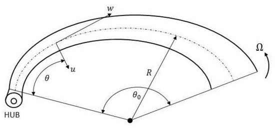
Figure 1. Geometry of a scimitar-type curved beam.

The equations of motion, when taking the effects of shear deformation and rotary inertia into account, are [29]:

$$\frac{\partial T\left(\theta ,t\right)}{\partial \theta }+N\left(\theta ,t\right)-\mu \left(\theta \right)R\frac{{\partial }^{2}u\left(\theta ,t\right)}{\partial t^2}=0,$$

(1)

$$\frac{\partial N\left(\theta ,t\right)}{\partial \theta }-T\left(\theta ,t\right)-\mu \left(\theta \right)R\frac{{\partial }^{2}w\left(\theta ,t\right)}{\partial t^2}=0,$$

(2)

$$\frac{\partial M\left(\theta ,t\right)}{\partial \theta }-RT\left(\theta ,t\right)=0,$$

(3)

where $T\left(\theta ,t\right)$ denotes the shear force, $N\left(\theta ,t\right)$ the normal force, $M\left(\theta ,t\right)$ the bending moment, $\mu \left(\theta \right)$ the mass per unit length ($\equiv \rho A\left(\theta \right)$) and $R$ the radius of the circular beam. The flexural deformations are more important than the axial deformation for the lowest modes of vibration [2], so that it is possible to neglect the extensibility of the beam’s neutral axis. The inextensibility condition is written as:

$$u=\frac{\partial w}{\partial \theta },$$

(4)

with the bending moment expressed as:

$$M\left(\theta ,t\right)=-\frac{EI\left(\theta \right)}{R^2}\left(\frac{{\partial }^{2}u}{\partial {\theta }^2}+u\right)=-\frac{EI\left(\theta \right)}{R^2}\left(\frac{{\partial }^{3}w}{\partial {\theta }^3}+\frac{\partial w}{\partial \theta }\right),$$

(5)

where $E$ is Young’s modulus, and $I\left(\theta \right)$ is the second moment of area. On substituting (5) into (3), an expression for the shear force is found:

$$T\left(\theta ,t\right)=-\frac{1}{R^3}\frac{\partial }{\partial \theta }\left[EI\left(\theta \right)\left(\frac{{\partial }^{3}w}{\partial {\theta }^3}+\frac{\partial w}{\partial \theta }\right)\right].$$

(6)

From (1) and (6), the following relation, identifying the normal force, is found:

$$\begin{array}{ll}N\left(\theta ,t\right)=-\frac{\partial T\left(\theta ,t\right)}{\partial \theta }& +\mu \left(\theta \right)R\frac{{\partial }^{2}u\left(\theta ,t\right)}{\partial t^2}\\ & =\frac{1}{R^2}\frac{{\partial }^2}{\partial {\theta }^2}\left[EI\left(\theta \right)\left(\frac{{\partial }^{3}w}{\partial {\theta }^3}+\frac{\partial w}{\partial \theta }\right)\right]+\mu \left(\theta \right)R\frac{{\partial }^{3}w\left(\theta ,t\right)}{\partial \theta \partial t}.\end{array}$$

(7)

By substitution the equation of motion for the deflection component, $w$ can be written as:

$$\begin{array}{c}\frac{{\partial }^3}{\partial {\theta }^3}\left[EI\left(\theta \right)\left(\frac{{\partial }^{3}w\left(\theta ,t\right)}{\partial {\theta }^3}+\frac{\partial w\left(\theta ,t\right)}{\partial \theta }\right)\right]+\frac{\partial }{\partial \theta }\left[EI\left(\theta \right)\left(\frac{{\partial }^{3}w\left(\theta ,t\right)}{\partial {\theta }^3}+\frac{\partial w\left(\theta ,t\right)}{\partial \theta }\right)\right]\\ +R^4\frac{\partial }{\partial \theta }\left[\mu \left(\theta \right)\frac{{\partial }^{3}w\left(\theta ,t\right)}{\partial \theta \partial t^2}\right]-\mu \left(\theta \right)R^4\frac{\partial w^2\left(\theta ,t\right)}{\partial t^2}=0.\end{array}$$

(8)

According to the modal analysis for the harmonic free vibration, $w\left(\theta ,t\right)$ can be separable in space and time as:

$$w\left(\theta ,t\right)=\phi \left(\theta \right)h\left(t\right),$$

(9)

where $\phi \left(\theta \right)$ is the modal deflection, and $h\left(t\right)$ is a harmonic function of time. If $\omega$ denotes the circular frequency of $h\left(t\right)$, then the eigenvalue problem of (8) is reduced to:

$$\frac{{\mathrm{d}}^3}{\mathrm{d}{\theta }^3}\left[EI\left(\theta \right)\left(\frac{{\mathrm{d}}^3\phi }{\mathrm{d}{\theta }^3}+\frac{\mathrm{d}\phi }{\mathrm{d}\theta }\right)\right]+\frac{\mathrm{d}}{\mathrm{d}\theta }\left[EI\left(\theta \right)\left(\frac{{\mathrm{d}}^3\phi }{\mathrm{d}{\theta }^3}+\frac{\mathrm{d}\phi }{\mathrm{d}\theta }\right)\right]-R^4{\omega }^2\left(\frac{\mathrm{d}}{\mathrm{d}\theta }\left[\mu \left(\theta \right)\frac{\mathrm{d}\phi }{\mathrm{d}\theta }\right]-\mu \left(\theta \right)\phi \right)=0.$$

(10)

Centrifugal stiffening occurs within rotors due to rotation and is given by:

$$T_s\left(\theta \right)=\underset{\theta }{\overset{{\theta }_0}{{\displaystyle \int }}}\left[\mu \left(\theta \right){\mathsf{\Omega }}^2(r_h+\theta \right]\mathrm{d}\theta ,$$

(11)

where $T_s$ is the centrifugal stiffening, $\mathsf{\Omega }$ is the angular rotating speed of the rotor, and $r_h$ is the offset length between the rotor and rotating hub center. For this work, the rotor is considered as a rotating beam without any offset, due to the presence of a hub, except for Figure 8 where the effect of the hub offset is considered. The governing equation for the tangential displacement of the beam becomes:

$$\begin{array}{c}\frac{{\mathrm{d}}^3}{\mathrm{d}{\theta }^3}\left[EI\left(\theta \right)\left(\frac{{\mathrm{d}}^3\phi }{\mathrm{d}{\theta }^3}+\frac{\mathrm{d}\phi }{\mathrm{d}\theta }\right)\right]+\frac{\mathrm{d}}{\mathrm{d}\theta }\left[EI\left(\theta \right)\left(\frac{{\mathrm{d}}^3\phi }{\mathrm{d}{\theta }^3}+\frac{\mathrm{d}\phi }{\mathrm{d}\theta }\right)\right]-R^4\frac{\mathrm{d}}{\mathrm{d}\theta }\left[T\left(\theta \right)\frac{\mathrm{d}\phi }{\mathrm{d}\theta }\right]\\ -R^4{\omega }^2\left(\frac{\mathrm{d}}{\mathrm{d}\theta }\left[\mu \left(\theta \right)\frac{\mathrm{d}\phi }{\mathrm{d}\theta }\right]-\mu \left(\theta \right)\phi \right)=0.\end{array}$$

(12)

3. Application of the AMDM

A flowchart is provided in the Appendix A to help the reader follow the various steps involved when using the Adomian modified decomposition method.

In order to simplify the analysis, the following parameters are introduced:

$$x=\theta /{\theta }_0, {\lambda }_1={\omega }^2\frac{\rho A_0{R}^4}{E{I}_0}, {\lambda }_2={\mathsf{\Omega }}^2\frac{\rho A_0{R}^4}{E{I}_0}.$$

(13)

Assuming a rectangular cross-section with a constant breath and linearly varying width, the cross-sectional area and moment of inertia can be expressed in general as:

$$\begin{gathered} A\left(x\right)=A_{0}a\left(x\right)=A_0{\left(1+\alpha \left(2x-1\right)\right)}^{r_1}, \\ I\left(x\right)=I_{0}b\left(x\right)=I_0{\left(1+\alpha \left(2x-1\right)\right)}^{r_2}, \end{gathered}$$

(14)

where $r_1$ and $r_2$ are real positive, $\alpha$ is the taper parameter, and $A_0$ and $I_0$ are the cross-sectional area and moment of inertia of the beam directly above the origin, as shown in Figure 2. This is the case for $r_1=1$ and $r_2=3$ and where the cross-sectional width is $h\left(x\right)=h_0\left(1+\alpha \left(2x-1\right)\right)$, with this case being used in the following development.

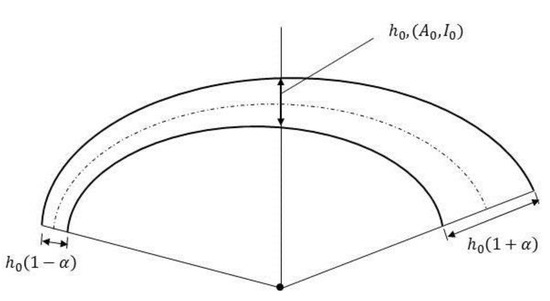
Figure 2. Linearly varying cross-sectional width of the curved beam.

Then, (12), together with (13) and (14), can be combined and expanded to give the following sixth-order differential equation:

$$\begin{array}{ll}{\phi }^{\prime \prime \prime \prime \prime \prime }+\frac{18\alpha }{a\left(x\right)}{\phi }^{\prime \prime \prime \prime \prime }& +\frac{2}{{\left(a\left(x\right)\right)}^2}\left[{\left(a\left(x\right){\theta }_0\right)}^2+36{\alpha }^2\right]{\phi }^{\prime \prime \prime \prime }+\frac{24\alpha }{b\left(x\right)}\left[{\left(a\left(x\right){\theta }_0\right)}^2+2{\alpha }^2\right]{\phi }^{‴}\\ & +{\left(\frac{{\theta }_0}{a\left(x\right)}\right)}^2\left[{\left(a\left(x\right){\theta }_0\right)}^2+72{\alpha }^2-{\lambda }_1{\theta }_0^2-{\lambda }_2\gamma {\theta }_0^2\right]{\phi }^{″}\\ & +\frac{2\alpha {\theta }_0^2}{b\left(x\right)}\left[3{\left(a\left(x\right){\theta }_0\right)}^2+24{\alpha }^2-{\lambda }_1{\theta }_0^2-{\lambda }_2{\gamma }^{\prime }{\theta }_0^2\right]{\phi }^{\prime }+\frac{{\theta }_0^6{\lambda }_1}{{\left(a\left(x\right)\right)}^2}\phi =0,\end{array}$$

(15)

where $\gamma =\frac{1}{6}\left(3+\alpha +3\left(\alpha -1\right)x^2-4\alpha x^3\right)$, and ${\phi }^{\prime }$ and ${\gamma }^{\prime }$ indicate a derivative w.r.t. x.

According to the AMDM, $\phi \left(x\right)$ in (15) can be expressed as an infinite series, i.e.:

$$\phi \left(x\right)={\displaystyle \sum }_{m=0}^{\infty }{C}_m{x}^m$$

(16)

where the unknown coefficients $C_m$ are determined recurrently. If a linear operator $G\equiv {\mathrm{d}}^6/\mathrm{d}{x}^6$ is used, then the inverse operator of $G$ is a six-fold integral operator defined as:

$$G^{-1}=\underset{0}{\overset{x}{{\displaystyle \int }}}\underset{0}{\overset{x}{{\displaystyle \int }}}\underset{0}{\overset{x}{{\displaystyle \int }}}\underset{0}{\overset{x}{{\displaystyle \int }}}\underset{0}{\overset{x}{{\displaystyle \int }}}\underset{0}{\overset{x}{{\displaystyle \int }}}(\cdots )\mathrm{d}x \mathrm{d}x \mathrm{d}x \mathrm{d}x \mathrm{d}x \mathrm{d}x \mathrm{d}x.$$

(17)

Then, (15) can now be written as:

$$\begin{array}{ll}\phi \left(x\right)=\mathsf{\Phi }\left(\mathrm{x}\right)+G^{-1}& \{\frac{-18\alpha }{a\left(x\right)}{\phi }^{\prime \prime \prime \prime \prime }-\frac{2}{{\left(a\left(x\right)\right)}^2}\left[{\left(a\left(x\right){\theta }_0\right)}^2+36{\alpha }^2\right]{\phi }^{\prime \prime \prime \prime }\\ & -\frac{24\alpha }{b\left(x\right)}\left[{\left(a\left(x\right){\theta }_0\right)}^2+2{\alpha }^2\right]{\phi }^{‴}\\ & -{\left(\frac{{\theta }_0}{a\left(x\right)}\right)}^2\left[{\left(a\left(x\right){\theta }_0\right)}^2+72{\alpha }^2-{\lambda }_1{\theta }_0^2-{\lambda }_2\gamma {\theta }_0^2\right]{\phi }^{″}\\ & -\frac{2\alpha {\theta }_0^2}{b\left(x\right)}\left[3{\left(a\left(x\right){\theta }_0\right)}^2+24{\alpha }^2-{\lambda }_1{\theta }_0^2-{\lambda }_2{\gamma }^{\prime }{\theta }_0^2\right]{\phi }^{\prime }-\frac{{\theta }_0^6{\lambda }_1}{{\left(a\left(x\right)\right)}^2}\phi ,\end{array}$$

(18)

where $\mathsf{\Phi }\left(x\right)={\displaystyle \sum }_{m=0}^5{C}_m{x}^m=\phi \left(0\right)+{\phi }^{\prime }\left(0\right)x+{\phi }^{″}\left(0\right)x^2/2!+\cdots +{\phi }^{\prime \prime \prime \prime \prime }\left(0\right)x^5/5!$.

To simplify the computational effort, use can be made of the Cauchy product, first by using a power series expansion to obtain:

$$\frac{1}{1+\alpha \left(2x-1\right)}={\displaystyle \sum }_{m=0}^{\infty }\frac{{\left(-1\right)}^k{\left(2\alpha \right)}^k}{{\left(1-\alpha \right)}^{k+1}}{x}^k={\displaystyle \sum }_{m=0}^{\infty }{\beta }_k{x}^k,$$

(19)

and then:

$$\frac{1}{{\left(1+\alpha \left(2x-1\right)\right)}^2}={\displaystyle \sum }_{m=0}^{\infty }{\beta }_k{x}^k{\displaystyle \sum }_{m=0}^{\infty }{\beta }_k{x}^k={\displaystyle \sum }_{m=0}^{\infty }{x}^k{\displaystyle \sum }_{j=0}^m{\beta }_{m-j}{\beta }_j={\displaystyle \sum }_{m=0}^{\infty }{\vartheta }_m{x}^m,$$

(20)

$$\frac{1}{{\left(1+\alpha \left(2x-1\right)\right)}^3}={\displaystyle \sum }_{m=0}^{\infty }{\beta }_k{x}^k{\displaystyle \sum }_{m=0}^{\infty }{\vartheta }_m{x}^m={\displaystyle \sum }_{m=0}^{\infty }{x}^k{\displaystyle \sum }_{j=0}^m{\beta }_{m-j}{\vartheta }_j={\displaystyle \sum }_{m=0}^{\infty }{\kappa }_m{x}^m.$$

(21)

By substituting the decomposition (16) into (18) and making use of (19)–(21) as alternatives for $a\left(x\right)$ and $b\left(x\right)$:

$$\begin{array}{ll}{\displaystyle {\displaystyle \sum }_{m=0}^{\infty }}{C}_m{x}^m=\mathsf{\Phi }\left(x\right)& \\ & +G^{-1}\{{\displaystyle {\displaystyle \sum }_{m=0}^{\infty }}{x}^m[-18\alpha {\displaystyle {\displaystyle \sum }_{j=0}^m}{\beta }_{m-j}\left(j+1\right)\left(j+2\right)\left(j+3\right)\left(j+4\right)(j+5)C_{j+5}\\ & -2{\theta }_0^2\left(m+1\right)\left(m+2\right)\left(m+3\right)\left(m+4\right)C_{m+4}\\ & -72{\alpha }^2{\displaystyle {\displaystyle \sum }_{j=0}^m}{\vartheta }_{m-j}\left(j+1\right)\left(j+2\right)\left(j+3\right)\left(j+4\right)C_{j+4}\\ & -24\alpha {\theta }_0^2{\displaystyle {\displaystyle \sum }_{j=0}^m}{\beta }_{m-j}\left(j+1\right)\left(j+2\right)\left(j+3\right)C_{j+3}\\ & -48{\alpha }^3{\displaystyle {\displaystyle \sum }_{j=0}^m}{\kappa }_{m-j}\left(j+1\right)\left(j+2\right)\left(j+3\right)C_{j+3}-{\theta }_0^4\left(m+1\right)\left(m+2\right)C_{m+2}\\ & -\left(72{\alpha }^2{\theta }_0^2-{\lambda }_1{\theta }_0^4-{\lambda }_2\gamma {\theta }_0^4\right){\displaystyle {\displaystyle \sum }_{j=0}^m}{\vartheta }_{m-j}\left(j+1\right)\left(j+2\right)C_{j+2}\\ & -6\alpha {\theta }_0^4{\displaystyle {\displaystyle \sum }_{j=0}^m}{\beta }_{m-j}\left(j+1\right)C_{j+1}\\ & -\left(48{\alpha }^3{\theta }_0^2-2{\lambda }_1\alpha {\theta }_0^4-2{\lambda }_2\alpha {\gamma }^{\prime }{\theta }_0^4\right){\displaystyle {\displaystyle \sum }_{j=0}^m}{\kappa }_{m-j}(j\\ & +1)C_{j+1}-{\theta }_0^6{\lambda }_1{\displaystyle {\displaystyle \sum }_{j=0}^m}{\vartheta }_{m-j}{C}_j]\}.\end{array}$$

(22)

On integrating, the following is obtained:

$$\begin{array}{ll}{\displaystyle {\displaystyle \sum }_{m=0}^{\infty }}{C}_m{x}^m=\phi \left(0\right)& +{\phi }^{\prime }\left(0\right)+{\phi }^{″}\left(0\right)\frac{x^2}{2!}+{\phi }^{‴}\left(0\right)\frac{x^3}{3!}+{\phi }^{\prime \prime \prime \prime }\left(0\right)\frac{x^4}{4!}+{\phi }^{\prime \prime \prime \prime \prime }\left(0\right)\frac{x^5}{5!}.\\ & +{\displaystyle {\displaystyle \sum }_{m=0}^{\infty }}\frac{x^{m+6}}{\left(m+1\right)\left(m+2\right)\left(m+3\right)\left(m+4\right)\left(m+5\right)\left(m+6\right)}\{-18\alpha {\displaystyle {\displaystyle \sum }_{j=0}^m}{\beta }_{m-j}(j\\ & +1)\left(j+2\right)\left(j+3\right)j+4)\left(j+5\right)C_{j+5}\\ & -2{\theta }_0^2\left(m+1\right)\left(m+2\right)\left(m+3\right)\left(m+4\right)C_{m+4}\\ & -72{\alpha }^2{\displaystyle {\displaystyle \sum }_{j=0}^m}{\vartheta }_{m-j}\left(j+1\right)\left(j+2\right)\left(j+3\right)\left(j+4\right)C_{j+4}\\ & -24\alpha {\theta }_0^2{\displaystyle {\displaystyle \sum }_{j=0}^m}{\beta }_{m-j}\left(j+1\right)\left(j+2\right)\left(j+3\right)C_{j+3}\\ & -48{\alpha }^3{\displaystyle {\displaystyle \sum }_{j=0}^m}{\kappa }_{m-j}\left(j+1\right)\left(j+2\right)\left(j+3\right)C_{j+3}-{\theta }_0^4\left(m+1\right)\left(m+2\right)C_{m+2}\\ & -\left(72{\alpha }^2{\theta }_0^2-{\lambda }_1{\theta }_0^4-{\lambda }_2\gamma {\theta }_0^4\right){\displaystyle {\displaystyle \sum }_{j=0}^m}{\vartheta }_{m-j}\left(j+1\right)\left(j+2\right)C_{j+2}\\ & -6\alpha {\theta }_0^4{\displaystyle {\displaystyle \sum }_{j=0}^m}{\beta }_{m-j}\left(j+1\right)C_{j+1}\\ & -\left(48{\alpha }^3{\theta }_0^2-2{\lambda }_1\alpha {\theta }_0^4-2{\lambda }_2\alpha {\gamma }^{\prime }{\theta }_0^4\right){\displaystyle {\displaystyle \sum }_{j=0}^m}{\kappa }_{m-j}\left(j+1\right)C_{j+1}-{\theta }_0^6{\lambda }_1{\displaystyle {\displaystyle \sum }_{j=0}^m}{\vartheta }_{m-j}{C}_j\}\end{array}$$

(23)

The recurrence relation for the coefficients $C_m$ can be stated as:

$$C_0=\phi \left(0\right), C_1={\phi }^{\prime }\left(0\right), C_2=\frac{{\phi }^{″}\left(0\right)}{2!}, C_3=\frac{{\phi }^{‴}\left(0\right)}{3!}, C_4=\frac{{\phi }^{\prime \prime \prime \prime }\left(0\right)}{4!}, C_5=\frac{{\phi }^{\prime \prime \prime \prime \prime }\left(0\right)}{5!},$$

(24)

and for $m\ge 6$, as:

$$\begin{array}{ll}{C}_m=\frac{1}{m\left(m-1\right)\left(m-2\right)\left(m-3\right)\left(m-4\right)\left(m-5\right)}& \{-18\alpha {\displaystyle {\displaystyle \sum }_{j=0}^{m-6}}{\beta }_{m-j-6}\left(j+1\right)\left(j+2\right)(j\\ & +3)j+4)\left(j+5\right)C_{j+5}-2{\theta }_0^2\left(m-5\right)\left(m-4\right)\left(m-3\right)\left(m-2\right)C_{m-2}\\ & -72{\alpha }^2{\displaystyle {\displaystyle \sum }_{j=0}^{m-6}}{\vartheta }_{m-j-6}\left(j+1\right)\left(j+2\right)\left(j+3\right)\left(j+4\right)C_{j+4}\\ & -24\alpha {\theta }_0^2{\displaystyle {\displaystyle \sum }_{j=0}^{m-6}}{\beta }_{m-j-6}\left(j+1\right)\left(j+2\right)\left(j+3\right)C_{j+3}\\ & -48{\alpha }^3{\displaystyle {\displaystyle \sum }_{j=0}^{m-6}}{\kappa }_{m-j-6}\left(j+1\right)\left(j+2\right)\left(j+3\right)C_{j+3}\\ & -{\theta }_0^4\left(m-5\right)\left(m-4\right)C_{m-4}\\ & -\left(72{\alpha }^2{\theta }_0^2-{\lambda }_1{\theta }_0^4-{\lambda }_2\gamma {\theta }_0^4\right){\displaystyle {\displaystyle \sum }_{j=0}^{m-6}}{\vartheta }_{m-j-6}\left(j+1\right)\left(j+2\right)C_{j+2}\\ & -6\alpha {\theta }_0^4{\displaystyle {\displaystyle \sum }_{j=0}^{m-6}}{\beta }_{m-j-6}\left(j+1\right)C_{j+1}\\ & -\left(48{\alpha }^3{\theta }_0^2-2{\lambda }_1\alpha {\theta }_0^4-2{\lambda }_2\alpha {\gamma }^{\prime }{\theta }_0^4\right){\displaystyle {\displaystyle \sum }_{j=0}^{m-6}}{\kappa }_{m-j-6}(j\\ & +1)C_{j+1}-{\theta }_0^6{\lambda }_1{\displaystyle {\displaystyle \sum }_{j=0}^{m-6}}{\vartheta }_{m-j-6}{C}_j\}.\end{array}$$

(25)

Therefore, the coefficients $C_m$ can be found from the recurrent (24) and (25), and the solution for $\phi \left(x\right)$ can calculated using (22). The series solution is $\phi \left(x\right)={\sum }_{m=0}^{\infty }{C}_m{x}^m$, but all of the coefficients $C_m$ cannot be determined, and so the solutions must be approximated by the truncated series ${\sum }_{m=0}^{n-1}{C}_m{x}^m$, with the successive approximations being ${\phi }^{\left[n\right]}={\sum }_{m=0}^{n-1}{C}_m{x}^m$ as $n$ increases and the boundary conditions are met.

Thus ${\phi }^{\left[1\right]}\left(x\right)=C_0, {\phi }^{\left[2\right]}\left(x\right)={\phi }^{\left[1\right]}\left(x\right)+C_{1}x, \cdots , {\phi }^{\left[5\right]}\left(x\right)= {\phi }^{\left[4\right]}\left(x\right)+C_4{x}^4$ serve as approximate solutions with an increasing accuracy as $n\to \infty$ and are also obligated to satisfy the boundary conditions, which are now discussed.

The boundary conditions for $\phi$, in the presence of constraints with the translational spring constants $k_{TL},k_{TR}$ and the rotational spring constants $k_{RL},k_{RR}$ (as shown on Figure 3), are given:

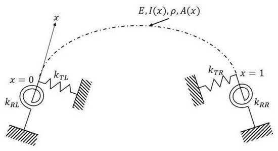
Figure 3. Scimitar-type curved beam with rotational and translational flexible ends.

For $x=0$:

$$EI\left(x\right)\frac{{\mathrm{d}}^2\phi \left(x\right)}{\mathrm{d}{x}^2}-K_{RL}\frac{\mathrm{d}\phi \left(x\right)}{\mathrm{d}x}=0, \frac{\mathrm{d}}{\mathrm{d}x}\left[EI\left(x\right)\frac{{\mathrm{d}}^2\phi \left(x\right)}{\mathrm{d}{x}^2}\right]+K_{TL}\phi \left(x\right)=0.$$

(26)

For $x=1$:

$$EI\left(x\right)\frac{{\mathrm{d}}^2\phi \left(x\right)}{\mathrm{d}{x}^2}+K_{RR}\frac{\mathrm{d}\phi \left(x\right)}{\mathrm{d}x}=0, \frac{\mathrm{d}}{\mathrm{d}x}\left[EI\left(x\right)\frac{{\mathrm{d}}^2\phi \left(0\right)}{\mathrm{d}{x}^2}\right]-K_{TR}\phi \left(x\right)=0.$$

(27)

On setting $I_1=I_0{\left(1+\alpha \right)}^3$ as the inertia at the free end of the beam, the coefficients can be written as:

$$k_{TL}=\frac{K_{TL}}{E{I}_0}, k_{TR}=\frac{K_{TR}}{E{I}_1}, k_{RL}=\frac{K_{RL}}{E{I}_0}, k_{RR}=\frac{K_{RR}}{E{I}_1}.$$

(28)

and the boundary conditions (26) and (27) can now be written as:

$$\begin{array}{l}\frac{{\mathrm{d}}^2\phi \left(0\right)}{\mathrm{d}{x}^2}-k_{RL}\frac{\mathrm{d}\phi \left(0\right)}{\mathrm{d}x}=0,\\ \frac{d^3\phi \left(0\right)}{d{x}^3}+6\alpha {\left(1-\alpha \right)}^2\frac{{\mathrm{d}}^2\phi \left(0\right)}{\mathrm{d}{x}^2}+k_{TL}\phi \left(0\right)=0,\\ \frac{{\mathrm{d}}^2\phi \left(1\right)}{\mathrm{d}{x}^2}+k_{RR}\frac{\mathrm{d}\phi \left(1\right)}{\mathrm{d}x}=0,\\ \frac{d^3\phi \left(1\right)}{d{x}^3}+6\alpha {\left(1+\alpha \right)}^2\frac{{\mathrm{d}}^2\phi \left(1\right)}{\mathrm{d}{x}^2}+k_{TL}\phi \left(1\right)=0.\end{array}$$

(29)

The six coefficients $C_m\left(m=0,1,2,\dots , 5\right)$ are decided by the boundary conditions of (29), with two of the coefficients $C_0$ and $C_1$ chosen as arbitrary constants, while the other three coefficients can be expressed as functions of $C_0$ and $C_1.$ Thus, from (24) and (29):

$$\begin{array}{l}{C}_2=\frac{k_{RL}}{2}{C}_1,\\ C_3=\frac{-6\alpha {\left(1-\alpha \right)}^2{k}_{RL}{C}_1-k_{TL}{C}_0}{6},\\ C_4=\frac{-36\alpha {\left(1-\alpha \right)}^2{C}_3+k_{TL}{C}_1}{24},\\ C_5=\frac{-144\alpha {\left(1-\alpha \right)}^2{C}_4+2k_{TL}{C}_2}{120}.\end{array}$$

(30)

The initial term $\mathsf{\Phi }\left(x\right)$ in (22) is a function of $C_0,C_1$, and from the recurrence relation of (25) the coefficients $C_m\left(m\ge 6\right)$ are functions of $C_0, C_1$ and ${\lambda }_1$. By substituting ${\phi }^{\left[n\right]}\left(x\right)$ into the last two equations of (29), i.e., for the free end of the beam, we then have:

$$f_{r0}^{\left[n\right]}\left({\lambda }_1\right)C_0+f_{r1}^{\left[n\right]}\left({\lambda }_1\right)C_1=0, r=1,2.$$

(31)

For nontrivial solutions of $C_0$ and $C_1,$ the frequency equation is given as:

$$\left|\begin{array}{cc}{f}_{10}^{\left[n\right]}\left({\lambda }_1\right)& f_{11}^{\left[n\right]}\left({\lambda }_1\right)\\ f_{20}^{\left[n\right]}\left({\lambda }_1\right)& f_{21}^{\left[n\right]}\left({\lambda }_1\right)\end{array}\right|=0.$$

(32)

The ith estimated eigenvalue ${\lambda }_{1\left(i\right)}^{\left[n\right]}$ corresponding to $n$ is obtained from (32), i.e., the ith estimated dimensionless natural frequency ${\mathsf{\Omega }}_{n\left(i\right)}^{\left[n\right]}=\sqrt{{\lambda }_{1\left(i\right)}^{\left[n\right]}}$ is obtained, and $n$ is determined by the following equation:

$$\left|{\mathsf{\Omega }}_{n\left(i\right)}^{\left[n\right]}-{\mathsf{\Omega }}_{n\left(i\right)}^{\left[n-1\right]}\le \epsilon \right|,$$

(33)

where ${\mathsf{\Omega }}_{n\left(i\right)}^{\left[n-1\right]}$ is the ith estimated dimensionless natural frequency corresponding to $n-1$, and $\epsilon$ is a preset and sufficiently small value. If (33) is satisfied, then ${\mathsf{\Omega }}_{n\left(i\right)}^{\left[n\right]}$ is the ith dimensionless natural frequency ${\mathsf{\Omega }}_{n\left(i\right)}$. By substituting ${\mathsf{\Omega }}_{n\left(i\right)}^{\left[n\right]}$ into (31), we obtain:

$$C_1=-\frac{f_{r0}^{\left[n\right]}\left({\mathsf{\Omega }}_{n\left(i\right)}^{\left[n\right]}\right)}{f_{r1}^{\left[n\right]}\left({\mathsf{\Omega }}_{n\left(i\right)}^{\left[n\right]}\right)}{C}_0, r=1,2,$$

(34)

and all of the other coefficients $C_m$ can be obtained from (24) and (25). Furthermore, the ith shape function ${\phi }_i^{\left[n\right]}$ corresponding to the ith eigenvalue ${\mathsf{\Omega }}_{n\left(i\right)}^{\left[n\right]}$ is obtained by:

$${\phi }_i^{\left[n\right]}\left(x\right)={\displaystyle \sum }_{m=0}^{n-1}{C}_m^{\left[i\right]}{x}^m,$$

(35)

where $C_m^{\left[i\right]}\left(x\right)$ is $C_m\left(x\right)$, in which ${\lambda }_1$ is substituted by ${\lambda }_{1\left(i\right)}$ and ${\phi }_i^{\left[n\right]}$ is the ith eigenfunction corresponding to the ith eigenvalue ${\lambda }_{1\left(i\right)}$. By normalizing (35), the ith normalized eigenfunction is defined as:

$${\overline{\phi }}_i^{\left[n\right]}\left(x\right)=\frac{{\phi }_i^{\left[n\right]}\left(x\right)}{\sqrt{{{\displaystyle \int }}_0^1{\left[{\phi }_i^{\left[n\right]}\left(x\right)\right]}^2\mathrm{d}x}},$$

(36)

where ${\overline{\phi }}_i^{\left[n\right]}\left(x\right)$ is the ith mode shape function of the beam corresponding to the ith natural frequency ${\omega }_i^{\left[n\right]}=\sqrt{{\lambda }_i^{\left[n\right]}}\sqrt{E{I}_0/\rho A_0{R}^4}={\mathsf{\Omega }}_{n\left(i\right)}^{\left[n\right]}\sqrt{E{I}_0/\rho A_0{R}^4}$.

4. Numerical Results

4.1. Unsymmetrical Nonrotating Arch

The AMDM was first partially validated using the unsymmetrical nonprismatic, nonrotating arch shown on Figure 2, whose cross-sectional height varies as $h_0\left(1+\alpha \left(2x-1\right)\right).$ In this example, the beam is considered as a clamped-free beam, so that $k_{RL}\to \infty , k_{TL}\to \infty , k_{RR}=0$ and $k_{RT}=0$. Furthermore, the beam is not rotating, so the terms in (15) involving $\mathsf{\Omega }$ are set to zero. The boundary conditions are:

$$\phi \left(0\right)=0, \frac{\mathrm{d}\phi \left(0\right)}{\mathrm{d}x}=0, \frac{{\mathrm{d}}^2\phi \left(1\right)}{\mathrm{d}{x}^2}=0, \frac{{\mathrm{d}}^3\phi \left(1\right)}{\mathrm{d}{x}^3}=0.$$

(37)

The coefficients $C_0$ and $C_1$ can be set to zero and the coefficients $C_2$ and $C_3$ set as arbitrary constants. The coefficients $C_4$ and $C_5$ are expressed in terms of $C_0$ and $C_1$ with the coefficients $C_m$ found from (25). By substituting ${\phi }^{\left[n\right]}={\displaystyle \sum }_{m=0}^{n-1}{C}_m{x}^m$ into the last two boundary conditions of (37), two algebraic equations involving $C_2$ and $C_3$ can be written as:

$${\displaystyle \sum }_{m=0}^{n-3}\left(m+1\right)\left(m+2\right)C_{m+2}=f_{12}^{\left[n\right]}\left({\lambda }_1\right)C_2+f_{13}^{\left[n\right]}\left({\lambda }_1\right)C_3=0$$

(38)

$${\displaystyle \sum }_{m=0}^{n-4}\left(m+1\right)\left(m+2\right)\left(m+3\right)C_{m+3}=f_{22}^{\left[n\right]}\left({\lambda }_1\right)C_2+f_{23}^{\left[n\right]}\left({\lambda }_1\right)C_3=0$$

(39)

For nontrivial solutions of $C_2$ and $C_3$, the frequency equation can be written as:

$$f_{12}^{\left[n\right]}\left({\lambda }_1\right)f_{23}^{\left[n\right]}\left({\lambda }_1\right)-f_{22}^{\left[n\right]}\left({\lambda }_1\right)f_{13}^{\left[n\right]}\left({\lambda }_1\right)=0$$

(40)

This problem has also been considered by Liu and Wu [5] and Karami and Malekzadeh [3], and the current results for dimensionless natural frequencies are compared with those of [5] in Table 1.

Table 1. Nondimensional natural frequencies for a nonrotating arch under clamped-free boundary conditions.

${\mathit{\theta }}_0 \left(\mathbf{deg}\right)$	AMDM	DQ [5]	Dev (%)	AMDM	DQ [5]	Dev (%)
${\mathsf{\Omega }}_{n\left(1\right)}$
	$\alpha =0.1$			$\alpha =0.2$
10	10.0834	10.0834	0	9.4062	9.4064	−0.002
20	5.0465	5.0465	0	4.7077	4.7078	−0.002
40	2.5328	2.5328	0	2.3631	2.3630	+0.004
60	1.6993	1.6993	0	1.5857	1.5856	+0.006
80	1.2858	1.2858	0	1.2000	1.1999	+0.008
${\mathsf{\Omega }}_{n\left(1\right)}$
	$\alpha =0.3$			$\alpha =0.4$
10	8.7089	8.7087	+0.002	7.9817	7.9805	+0.015
20	4.3588	4.3586	+0.005	3.9951	3.9943	+0.020
40	2.1582	2.1580	+0.009	2.0059	2.0053	+0.030
60	1.4685	1.4683	+0.014	1.3466	1.3460	+0.045
80	1.1117	1.1115	+0.018	1.0194	1.0191	+0.030
${\mathsf{\Omega }}_{n\left(2\right)}$
	$\alpha =0.1$			$\alpha =0.2$
10	26.3098	26.3097	+0.0004	25.7092	25.7091	+0.0003
20	13.0809	13.0808	+0.0008	12.7757	12.7756	+0.0008
40	6.4038	6.4038	0	6.2430	6.2429	+0.0016
60	4.1398	4.1399	−0.002	4.0264	4.0263	+0.0025
80	2.9956	2.9955	+0.003	2.9064	2.9062	+0.0067
${\mathsf{\Omega }}_{n\left(2\right)}$
	$\alpha =0.3$			$\alpha =0.4$
10	25.0359	25.0358	+0.0004	24.2758	24.2742	+0.0066
20	12.4340	12.4338	+0.0016	12.0487	12.0479	+0.0066
40	6.0640	6.0638	+0.0033	5.8629	5.8625	+0.0068
60	3.9009	3.9007	+0.0051	3.7610	3.7608	+0.0053
80	2.8089	2.8086	+0.0106	2.7010	2.7005	+0.0185

In the above table, the AMDM results are from the present method and the DQ results are those reported by Ref. [5]. It can be seen that, for the taper parameter $\alpha$ up to 0.3, there is very little difference in the two sets of results, but that for $\alpha =0.4,$ the respective sets of results begin to vary with the present natural frequencies calculated as being slightly higher. At this value of $\alpha$, the height ratio of the two ends of the arch is $\left(1+\alpha \right)/\left(1-\alpha \right)=2.\dot{3}$, which is a significant variation, and the results of Table 1 indicate an increasing deviation between the two sets of results as $\alpha$ increases.

In Table 2 and Table 3, the results calculated with the current method are compared with those from Ref. [3] calculations for the nonrotating unsymmetrical arch for different slenderness ratios $\left(S=\left(R{\theta }_0/\sqrt{I_0/A_0}\right)\right)$ for the two sets of boundary conditions clamped-free and simple-free. For the simple-free boundary conditions, the following are set for (29): $k_{RL}=\infty , k_{TL}\to \infty , k_{RR}=0$ and $k_{RT}=0$. At up to two decimal places, the results are identical, but when the third and fourth decimal places are considered, there is at times a large variation. The variation between the two sets of results gets larger with the higher modes and also generally as the slenderness ratio increases.

Table 2. The first four nondimensional natural frequencies $({\mathsf{\Omega }}_{n\left(i\right)}$) for a nonrotating arch $\left({\theta }_0=90°\right)$ against the slender ratio $S=\left(R{\theta }_0/\sqrt{I_0/A_0}\right)$ and under clamped-free boundary conditions.

S	$\alpha =0.2$
	AMDM	DQ [3]	Dev (%)	AMDM	DQ [3]	Dev (%)
	${\mathsf{\Omega }}_{n\left(1\right)}$			${\mathsf{\Omega }}_{n\left(2\right)}$
10	1.0704	1.0705	−0.0093	2.2911	2.2905	0.0262
20	1.0718	1.0720	−0.0186	2.4867	2.4854	0.0523
40	1.0722	1.0724	−0.0186	2.5228	2.5220	0.0317
100	1.0723	1.0725	−0.0186	2.5321	2.5311	0.0395
200	1.0724	1.0725	−0.0093	2.5334	2.5323	0.0434
400	1.0724	1.0725	−0.0093	2.5340	2.5327	0.0513
1000	1.0724	1.0725	−0.0093	2.5341	2.5328	0.0513
4000	1.0724	1.0725	−0.0093	2.5341	2.5328	0.0513
	${\mathsf{\Omega }}_{n\left(3\right)}$			${\mathsf{\Omega }}_{n\left(4\right)}$
10	3.0401	3.0399	0.0066	4.3598	4.3602	−0.0092
20	3.8912	3.8907	0.0129	4.8401	4.8671	−0.5547
40	4.5823	4.5818	0.0109	5.7111	5.7200	−0.1556
100	4.6669	4.6660	0.0193	6.7050	6.7160	−0.1638
200	4.6739	4.6736	0.0064	6.7398	6.7427	−0.0430
400	4.6757	4.6754	0.0064	6.7401	6.7454	−0.0786
1000	4.6758	4.6756	0.0043	6.7456	6.7489	−0.0488
4000	4.6758	4.6760	−0.0043	6.7467	6.7491	−0.0356
	$\alpha =0.4$
	${\mathsf{\Omega }}_{n\left(1\right)}$			${\mathsf{\Omega }}_{n\left(2\right)}$
10	0.9102	0.9100	0.0220	2.1468	2.1464	0.0186
20	0.9111	0.9109	0.0219	2.3069	2.3065	0.0173
40	0.9113	0.9111	0.0219	2.3391	2.3385	0.0256
100	0.9114	0.9112	0.0219	2.3476	2.3467	0.0384
200	0.9114	0.9112	0.0219	2.3483	2.3478	0.0213
400	0.9114	0.9112	0.0219	2.3483	2.3481	0.0085
1000	0.9114	0.9112	0.0219	2.3483	2.3481	0.0085
4000	0.9114	0.9112	0.0219	2.3483	2.3481	0.0085
	${\mathsf{\Omega }}_{n\left(3\right)}$			${\mathsf{\Omega }}_{n\left(4\right)}$
10	2.9215	2.9211	0.0137	4.3236	4.3228	0.0185
20	3.7675	3.7669	0.0159	4.7479	4.7467	0.0253
40	4.4269	4.4262	0.0158	5.5915	5.5908	0.0125
100	4.5160	4.5153	0.0155	6.5627	6.5618	0.0137
200	4.5243	4.5237	0.0133	6.5904	6.5899	0.0076
400	4.5269	4.5256	0.0287	6.5981	6.5951	0.0455
1000	4.5278	4.5261	0.0376	6.5989	6.5964	0.0380
4000	4.5283	4.5263	0.0442	6.5992	6.5967	0.0379

Table 3. The first four nondimensional natural frequencies $({\mathsf{\Omega }}_{n\left(i\right)}$) for a nonrotating arch $\left({\theta }_0=90°\right)$ against the slender ratio $S=\left(R{\theta }_0/\sqrt{I_0/A_0}\right)$ and under simple-free boundary conditions.

S	$\alpha =0.2$
	AMDM	DQ [3]	Dev (%)	AMDM	DQ [3]	Dev (%)
	${\mathsf{\Omega }}_{n\left(1\right)}$			${\mathsf{\Omega }}_{n\left(2\right)}$
10	2.0366	2.0368	−0.0098	2.9081	2.9076	0.0172
20	2.0905	2.0907	−0.0096	3.8750	3.8743	0.0180
40	2.1014	2.1016	−0.0095	4.1963	4.1956	0.0167
100	2.1045	2.1045	0	4.2241	4.2236	0.0118
200	2.1047	2.1049	−0.0095	4.2272	4.2266	0.0142
400	2.1049	2.1050	−0.0048	4.2278	4.2273	0.0118
1000	2.1049	2.1050	−0.0048	4.2279	4.2275	0.0095
4000	2.1049	2.1050	−0.0048	4.2279	4.2276	0.0071
	${\mathsf{\Omega }}_{n\left(3\right)}$			${\mathsf{\Omega }}_{n\left(4\right)}$
10	4.1621	4.1619	0.0048	4.6155	4.6160	−0.0108
20	4.4472	4.4466	0.0135	6.2216	6.2220	−0.0064
40	5.7189	5.7184	0.0087	6.4123	6.4127	−0.0062
100	6.2838	6.2832	0.0095	8.2643	8.2648	−0.0060
200	6.2935	6.2930	0.0079	8.3163	8.3169	−0.0072
400	6.2954	6.2950	0.0064	8.3218	8.3220	−0.0024
1000	6.2958	6.2955	0.0048	8.3230	8.3232	−0.0024
4000	6.2958	6.2956	0.0032	8.3232	8.3234	−00024
	$\alpha =0.4$
	${\mathsf{\Omega }}_{n\left(1\right)}$			${\mathsf{\Omega }}_{n\left(2\right)}$
10	1.9122	1.9121	0.0052	2.8262	2.8258	0.0141
20	1.9645	1.9645	0	3.7478	3.7475	0.0080
40	1.9758	1.9757	0.0051	4.0866	4.0861	0.0122
100	1.9788	1.9786	0.0100	4.1211	4.1208	0.0073
200	1.9792	1.9791	0.0050	4.1251	4.1246	0.0121
400	1.9793	1.9792	0.0051	4.1257	4.1255	0.0048
1000	1.9793	1.9792	0.0051	4.1259	4.1258	0.0024
4000	1.9793	1.9792	0.0051	4.1259	4.1258	0.0024
	${\mathsf{\Omega }}_{n\left(3\right)}$			${\mathsf{\Omega }}_{n\left(4\right)}$
10	4.1111	4.1108	0.0073	4.5748	4.5746	0.0044
20	4.3849	4.3841	0.0182	6.1583	6.1585	−0.0032
40	5.5899	5.5894	0.0089	6.3112	6.3118	−0.0095
100	6.1674	6.1670	0.0065	8.1102	8.1100	0.0025
200	6.1791	6.1784	0.0113	8.1724	8.1728	−0.0049
400	6.1813	6.1807	0.0097	8.1793	8.1788	0.0061
1000	6.1820	6.1814	0.0097	8.1810	8.1802	0.0098
4000	6.1823	6.1815	0.0129	8.1812	8.1805	0.0086

A typical convergence of the AMDM is shown in Figure 4 for the first two natural frequencies. The case that is shown is for ${\theta }_0=60°$ and $\alpha =0.3$. Acceptable results can be seen with ${\mathsf{\Omega }}_{n\left(1\right)}$ converging after about 40 iterations and ${\mathsf{\Omega }}_{n\left(2\right)}$ after about 60 iterations. Generally, it was found that for higher modes more iterations were necessary.

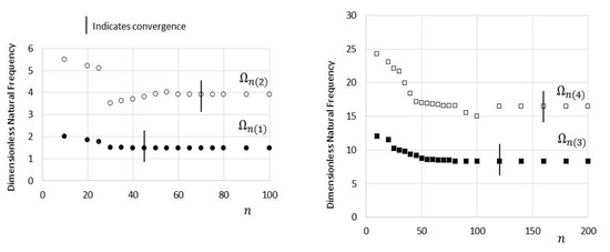
Figure 4. Convergence plots for the first two dimensionless natural frequencies (nonrotating).

4.2. Unsymmetrical Rotating Scimitar-Type Curved Beam

This section investigates the characteristics of a scimitar-type beam for different taper parameters and rotating speeds. An analysis using the absolute error remainder function and maximal error remainder [23,24] is also given in an effort to quantify the accuracy of the AMDM approach.

The results here are limited to a maximum of ${\theta }_0=80°$ because the trends found with these lower values of ${\theta }_0$ simply continued for higher values and because, secondly, values up to $80°$ constitute the region of interest in this work, as eventually the calculations are to be used in the design of propeller blades for prop-fan engines. For values above $80°,$ it may well be that a sudden change in the beam cross-section and/or material density, causing a discrete discontinuity in the beam parameters, may be necessary for aerodynamic and acoustic reasons.

The first and second natural frequencies, at different rotating speeds $\left({\lambda }_2\right)$ and with different taper parameter $\left(\alpha \right)$ and opening angle ${\theta }_0$ values, are shown on Figure 5 and Figure 6. Generally, there is a consistent rise in the natural frequency values with the rotation speed for all the taper parameters and opening angles that are tested. For the first natural frequencies, it can be seen that, at ${\theta }_0=40°,$ the increase when $\alpha =0.4$ is substantially greater than when $\alpha =0.1.$ This pattern is repeated for ${\theta }_0=80°$. It can be also seen that the values for the first natural frequency increase at a faster rate with the rotation speed for each equivalent value of $\alpha$ when the value of ${\theta }_0$ is greater.

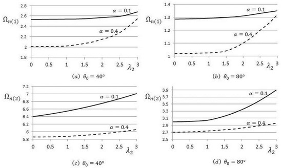
Figure 5. First and second natural frequencies’ variations with the rotation speed $\left({\lambda }_2\right)$ for different taper parameter $\left(\alpha \right)$ and opening angle $\left({\theta }_0\right)$ values.

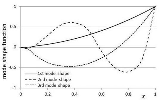
Figure 6. The first three mode shape functions, with ${\theta }_0=60°$, ${\lambda }_2=1.0$ and $\alpha =0.2.$

For the second natural frequency, an increase with the rotation speed is again generally found. In this case, the trend of an increase with the taper parameter is reversed in that for both ${\theta }_0=40°$ and ${\theta }_0=60°$ the increase is much more substantial when $\alpha =0.4$ rather than $\alpha =0.1$. Additionally, for each equivalent value of $\alpha ,$ the increase in values when ${\theta }_0=40°$ is greater when compared to ${\theta }_0=80°$.

The first three mode shapes for ${\theta }_0=60°$, ${\lambda }_2=1.0$ and $\alpha =0.2$ are shown in Figure 6 using the nondimensional form shown in (36). Variations of the first mode shape with the taper parameter and with the opening angle are shown in Figure 7. The mode shape is shown to deepen as both $\alpha$ and ${\theta }_0$ increase, as indicated by the arrows.

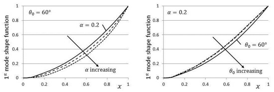
Figure 7. Variation of the first mode shape function, with ${\lambda }_2=1.0$.

The effect that the variation of the hub radius parameter has on the first frequency parameter is shown in Figure 8. It can be clearly seen that an increase in the hub offset has a considerable effect on the first frequency, especially at higher rotation speed values. The first frequency generally increases with the hub radius.

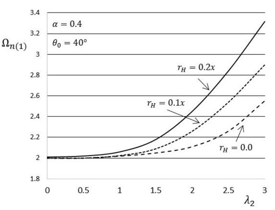
Figure 8. Effect of the hub radius parameter on the first frequency.

In this investigation, the accuracy of the present method is examined using the absolute error remainder functions and the maximal error remainder parameters, as defined for the current model (see (15)):

$$\left|E_n\left(x\right)\right|=\left|L{\phi }_i^{\left[n\right]}\left(x\right)+R{\phi }_i^{\left[n\right]}\left(x\right)\right|,$$

(41)

$$ME{R}_n=\underset{0\le x\le 1}{\max }\left|E{R}_n\left(x\right)\right|.$$

(42)

Here, $L$ is an invertible operator, which is taken as the highest-order derivative, $R$ is the remainder of the linear operation of (15), $\left|E_n\left(x\right)\right|$ is plotted against $x$ for each approximation of ${\phi }_i^{\left[n\right]}$ and $ME{R}_n$ is plotted against the index $n$. One of the native commands in Mathematica [30] is used here, i.e., NMaximize.

In Figure 9, it can be noted that the absolute error remainder values steadily decrease along the length of the beam, with very little movement noted between $n=60$ and $n=70.$ In Figure 10, the maximal error remainder parameter $ME{R}_{70}$ is just above ${10}^{-4},$ and it is noted that between $n=40$ and $n=70$ the points indicate a reasonably linear decrease, indicating an approximately exponential rate of convergence.

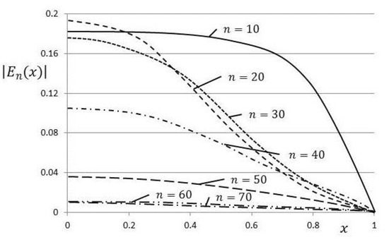
Figure 9. The curves of the absolute error remainder functions.

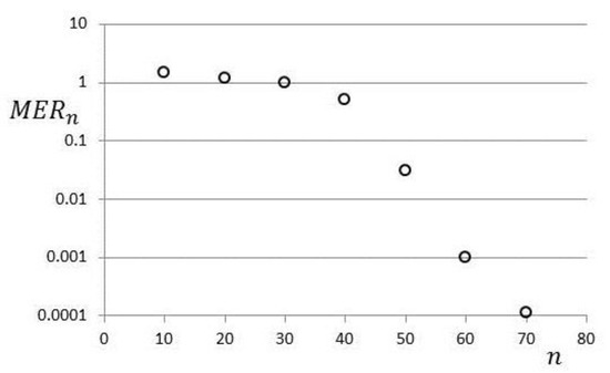
Figure 10. Logarithmic plot of the maximal error remainder parameters $ME{R}_n$.

5. Conclusions

The governing differential equation of motion for a scimitar-type rotating curved beam undergoing free natural vibration and rotation was derived using the Euler−Bernoulli formulation, and subsequently the Adomian modified decomposition technique was used for the resulting equation’s solution and boundary conditions. The Adomian modified decomposition method proved to be a highly effective and efficient method of obtaining the closed-form series solutions of the free vibrations of a rotating scimitar-type beam with flexible ends. Once the coding was written for the governing equations and boundary conditions, which were written compactly using coefficients which could be given zero or infinity, it was relatively simply to change from one type of boundary condition to another. The ith natural frequency and mode shape function can be derived using this method, and based on the current work there is good reason to say that this method, though limited to one type of beam, gives similar results for other, more complicated, schemes. Although not shown in this work, the possibility of extending the AMDM to nonlinear equations is also very appealing.

Numerical results for the natural frequencies were obtained for both a nonrotating arch and a rotating beam, with a good agreement found with the few solutions available in the literature. Two decisive advantages in using the AMDM are its fast convergence rate to the solution and the high degree of accuracy of the solution. The natural frequencies that are obtained are in good agreement with the published results. Compared to the results of the generalized differential quadrature rule used by several authors in the literature, the AMDM method was found to calculate the natural frequencies of nonrotating beams at slightly higher values, although overall the percentage deviation was very low for all results. In addition to the clamped-free boundary conditions that were suitable for propeller investigations, some calculations were performed for simple-free boundary conditions. Here, as with the clamped-free boundary conditions, the variation between the current and published calculations gets higher with a higher mode and slenderness ratio.

There was a consistent rise in the natural frequency with the rotational speed for all the taper parameters and opening angles that were tested, both for the first and second frequencies. Regarding the mode shape, it was found to deepen as both the taper parameter and opening angle increased. The effect of adding the hub radius to the governing equation was quite substantial, with a considerable effect found on the profile of the first frequency.

Lastly, the accuracy of the present method was investigated using a novel method. The absolute error remainder values steadily decreased along the length of the beam until almost reaching zero, while the maximal error remainder parameter showed a fairly linear decrease, indicating an approximate exponential rate of convergence.

References

- Auciello, N.M.; De Rosa, M.A. Free vibration of circular arches: A review. J. Sound Vib. 1994, 176, 433–458. [Google Scholar] [CrossRef]
- Tong, X.; Mrad, N.; Tabarrok, B. n-plane vibration of circular arches with variable cross-sections. J. Sound Vib. 1998, 212, 121–140. [Google Scholar] [CrossRef]
- Karami, G.; Malekzadeh, G.P. In-plane free vibration analysis of circular arches with varying cross-sections using differential quadrature method. J. Sound Vib. 2004, 274, 777–799. [Google Scholar] [CrossRef]
- Chen, C.N. DQEM analysis of in-plane vibration of curved beam structures. Adv. Eng. Softw. 2005, 36, 412–424. [Google Scholar] [CrossRef]
- Liu, G.R.; Wu, T.Y. In-plane vibration analyses of circular arches by the generalized differential quadrature rule. Int. J. Mech. Sci. 2001, 43, 2597–2611. [Google Scholar] [CrossRef]
- Gimena, F.N.; Gonzaga, P.; Gimena, P.L. 3D-curved beam element with varying cross-sectional area under generalized loads. Eng. Struct. 2008, 30, 404–411. [Google Scholar] [CrossRef]
- Molari, L.; Ubertini, F. A flexibility-based finite element for linear analysis of arbitrarily curved arches. Int. J. Numer. Methods Eng. 2006, 65, 1333–1353. [Google Scholar] [CrossRef]
- Hodges, D.J.; Rutkowski, M.J. Free vibration analysis of rotating beams by a variable order finite element method. AIAA J. 1981, 19, 1459–1466. [Google Scholar] [CrossRef]
- Wright, D.A.; Smith, C.E.; Thresher, R.W.; Wang, J.L.C. Vibration modes of centrifugally stiffened beams. J. Appl. Mech. 1982, 49, 197–201. [Google Scholar] [CrossRef]
- Naguleswaran, S. Lateral vibration of a centrifugally tensioned uniform Euler-Bernoulli beam. J. Sound Vib. 1994, 176, 613–624. [Google Scholar] [CrossRef]
- Yoo, H.H.; Shin, S.H. Vibration analysis of cantilever beams. J. Sound Vib. 1998, 212, 807–828. [Google Scholar] [CrossRef]
- Mao, Q. Application of Adomain modified decomposition method to free vibration analysis of rotating beams. Math. Probl. Eng. 2013, 284720. [Google Scholar]
- Hsu, J.-C.; Lai, H.-Y.; Chen, C.K. An innovative eigenvalue problem solver for free vibration of uniform Timoshenko beams using the Adomian modified decomposition method. J. Sound Vib. 2009, 325, 451–470. [Google Scholar] [CrossRef]
- Adair, D.; Jaeger, M. Simulation of tapered rotating beams with centrifugal stiffening using the Adomian decomposition method. Appl. Math. Model. 2016, 40, 3230–3241. [Google Scholar] [CrossRef]
- Adair, D.; Jaeger, M. Vibration analysis of a uniform pre-twisted rotating Euler-Bernoulli beam using the modified Adomian decomposition method. Math. Mech. Solids 2018, 23, 1345–1363. [Google Scholar] [CrossRef]
- Wang, G.; Wereley, N.M. Free vibration analysis of rotating blades with uniform tapers. AIAA J. 2004, 42, 2429–2437. [Google Scholar] [CrossRef]
- Adair, D.; Jaeger, M. A power series solution for rotating non-uniform Euler-Bernoulli cantilever beams. J. Vib. Control 2018, 24, 3855–3864. [Google Scholar] [CrossRef]
- Banerjee, J.R.; Su, H.; Jackson, D.R. Free vibration of rotating tapered beams using the dynamic stiffness method. J. Sound Vib. 2006, 298, 1034–1054. [Google Scholar] [CrossRef]
- Özdemir, Ö.O.; Kaya, M.O. Flapwise bending vibration analysis of a rotating tapered cantilever Bernoulli-Euler beam by differential transform method. J. Sound Vib. 2006, 289, 413–420. [Google Scholar] [CrossRef]
- Gunda, J.B.; Ganguli, R. Stiff-string basis function for vibration analysis of high speed rotating beams. J. Appl. Mech. 2008, 75, 245021–245025. [Google Scholar] [CrossRef]
- Yang, X.D.; Li, Z.; Zhang, W.; Yang, T.Z.; Lin, C.W. On the gyroscopic and centrifugal effects in the free vibration of rotating beams. J. Vib. Control 2019, 25, 219–227. [Google Scholar] [CrossRef]
- Chen, Q.; Du, J. A Fourier series solution for the transverse vibration of rotating beams with elastic boundary supports. Appl. Acoustics 2019, 155, 1–15. [Google Scholar] [CrossRef]
- Qin, Y.; Li, X.; Yang, E.C.; Li, Y.H. Flapwise free vibration characteristics of a rotating composite thin-walled beam under aerodynamic force and hygrothermal environment. Comp. Struct. 2016, 153, 490–503. [Google Scholar] [CrossRef]
- Jokar, H.; Mahzoon, M.; Vatankhah, R. Dynamic modeling and free vibration analysis of horizontal axis wind turbine blades in the flap-wise direction. Ren. Ener. 2020, 146, 1818–1832. [Google Scholar] [CrossRef]
- Adomian, G. Solving Frontier Problems of Physics: The Decomposition Method; Kluwer Academic Publishers: Boston, MA, USA, 1994. [Google Scholar]
- Das, S. A numerical solution of the vibration equation using modified decomposition method. J. Sound Vib. 2009, 320, 576–583. [Google Scholar] [CrossRef]
- Rach, R.; Duan, J.S.; Wazwaz, A.M. On the solution of non-isothermal reaction-diffusion model equations in a spherical catalyst by the modified Adomian method. Chem. Eng. Commun. 2015, 202, 1081–1088. [Google Scholar] [CrossRef]
- Rach, R.; Duan, J.S.; Wazwaz, A.M. Simulation of large deflections of a flexible cantilever beam fabricated from functionally graded materials by the Adomian decomposition method. Int. J. Dyn. Syst. Differ. Equ. 2019. [Google Scholar] [CrossRef]
- Henrych, J. Dynamics of Arches and Frames; Elsevier: Amsterdam, The Netherlands, 1981. [Google Scholar]
- Wolfram Research Inc. Mathematica, Version 12.0; Wolfram Research Inc.: Champaign, IL, USA, 2019. [Google Scholar]
Publisher’s Note: MDPI stays neutral with regard to jurisdictional claims in published maps and institutional affiliations. |
© 2020 by the authors. Licensee MDPI, Basel, Switzerland. This article is an open access article distributed under the terms and conditions of the Creative Commons Attribution (CC BY) license (http://creativecommons.org/licenses/by/4.0/).