Numerical Approach to a Nonlocal Advection-Reaction-Diffusion Model of Cartilage Pattern Formation

Abstract

We propose a numerical approach that combines a radial basis function (RBF) meshless approximation with a finite difference discretization to solve a nonlinear system of integro-differential equations. The equations are of advection-reaction-diffusion type modeling the formation of pre-cartilage condensations in embryonic chicken limbs. The computational domain is four dimensional in the sense that the cell density depends continuously on two spatial variables as well as two structure variables, namely membrane-bound counterreceptor densities. The biologically proper Dirichlet boundary conditions imposed in the semi-infinite structure variable region is in favor of a meshless method with Gaussian basis functions. Coupled with WENO5 finite difference spatial discretization and the method of integrating factors, the time integration via method of lines achieves optimal complexity. In addition, the proposed scheme can be extended to similar models with more general boundary conditions. Numerical results are provided to showcase the validity of the scheme.

1. Introduction

A central question in several areas of biology is how populations of cells interact to form various complex structures. Examples include organogenesis in developmental biology [1,2] or tumor growth in cancer research [3,4]. These phenomena typically span several spatial and temporal scales and involve interactions of many different processes, such as undirected or directed cell motion, cell-cell adhesion, gene expression and the transport of various molecules by diffusion or advection.

Mathematical models have played an important role in the investigation of the underlying cellular and molecular mechanisms of these phenomena. In the framework of PDEs, coupled systems of advection-reaction-diffusion equations are often used. Several modeling approaches for cell-cell adhesion have been proposed in this continuous framework [5,6,7,8], the most widely adopted being that of Armstrong et al. [5] based on a nonlocal adhesion flux term. Most prominently, this has been applied in the area of tumor modeling and cancer invasion, see, e.g., [9,10,11,12,13,14,15]. A similar approach was also used to model the formation of liver cell aggregations in vitro [16].

In this paper, we study an advection-reaction-diffusion system modeling the formation of cell aggregations in cultures of embryonic chicken limbs proposed in [17]. These aggregations, also called pre-cartilage condensations, occur in vivo in the limb bud in early stages of development and lay down the precursors for the skeleton. The model contains nonlocal advection and reaction terms and is effectively four dimensional, with two spatial dimensions and two additional dimensions given by two structure variables on which the cell density depends.

High dimensionality is somewhat typical of models describing the interaction of cell populations. Indeed, it is often necessary to consider not only two or three spatial dimensions, but also additional structure variables for the cell population, such as cell age (modeled together with cell-cell adhesion in [18] and with haptotaxis, e.g., in [19]), or cell size [20]. Taking into account the nonlocal advection terms and the nonlinearity of the reaction terms, as well as the stiffness from highly distinct diffusivities, the numerical simulation of these models is challenging. In fact, due to the computational expense of the model in [17], the original paper only considered numerical solutions in one spatial dimension using a Lax–Friedrichs finite difference scheme. For a thorough computational analysis in the proper biological setting with two spatial dimensions, more sophisticated numerical methods are needed. This is the motivation of this work.

In the rest of this section, we will briefly describe the model from [17], followed by an introduction of the corresponding numerical approach.

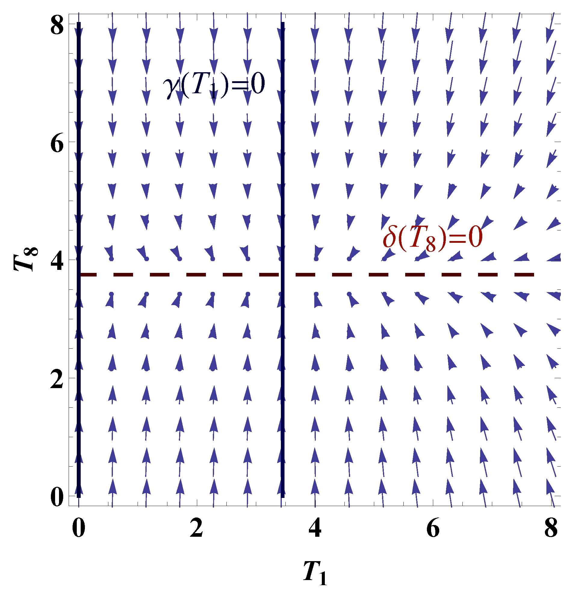
1.1. Mathematical Model

During early limb development in vertebrates, a template for the skeletal structure is laid out via the aggregation of mesenchymal cells as the first step of chondrogenesis, the formation of cartilage. These cells form tight aggregations called pre-cartilage condensations. At later stages, these condensations differentiate into cartilage, and much later typically into bone. This process can be observed in cell cultures as well. For this, chicken or mouse mesenchymal cells are extracted from early limb buds, mixed and plated as in vitro cultures, so-called high density micromass cultures. In these cultures, cells spontaneously form tight aggregations just like in vivo [21,22,23]. Indeed it is widely accepted that this process recapitulates the process of pre-cartilage condensation formation in vivo [24]. The aggregations in micromass experiments show a variety of morphologies, ranging from spot-like to labyrinth-like patterns, depending on whether the cells were taken from hind or front limbs, as well as various other parameters of the experiments [23]. Very important among these is the initial density of cells with lower cell densities producing spot-like patterns and higher densities producing stripe-like or labyrinth-like patterns [25]. See Figure 1 for some examples from the experimental literature.

Several mathematical models have been proposed to uncover the mechanism by which pre-cartilage condensations form (see reviews [28,29,30,31,32] and the papers cited therein). Of special interest have been reaction-diffusion type models which give rise to patterns via Turing-type mechanisms, e.g., the recently suggested BSW model [33].

In [17], the authors propose a model of limb chondrogenesis based on experimental work uncovering the role of a network of galectins in in vitro cultures of chicken mesenchyme [34]. Galectins are a class of sugar binding proteins. Galectins can promote or inhibit cell-cell adhesion, a crucial process for the formation of cell aggregations. Galectins are not membrane-bound, but diffuse freely throughout the extracellular matrix. They bind to membrane-bound proteins called counterreceptors. There is a complex interaction between galectins bound to counterreceptors and the production of galectins by cells.

In short, there are two galectins, CG (Chicken Galectin)-1A and CG-8, and two counterreceptors, CR-1 and CR-8. CG-1A may bind to CR-1; the complex induces the production of CG-8 and also crucially mediates cell-cell adhesion. The complex of CG-8 with its counterreceptor CR-8 induces the production of CG-1A, so that the two galectins effectively give rise to a positive feedback loop. However, CG-8 can also bind to the counterreceptor CR-1, thus ’blocking’ these for CG-1A. So somewhat paradoxically, an increase of CG-8 leads to fewer condensations while an increase of CG-1A, enhancing cell-cell adhesion, leads to more and tighter condensations. (See [34] for further details about the biochemical interactions.)

To elucidate this complex interaction, the following mathematical model was proposed in [17]:

$$\begin{array}{cc}\hfill \frac{\partial R}{\partial t}=& d_R{\nabla }_{\mathbf{x}}^{2}R-{\nabla }_{\mathbf{x}}·\left(R\mathbf{K}\left(R\right)\right)-\frac{\partial }{\partial T_1}\left(\tilde{\gamma }(c_1^u,c_8^u,T_1)R\right)-\frac{\partial }{\partial T_8}\left(\tilde{\delta }(c_8^u,T_8)R\right)\hfill \end{array}$$

(1)

$$\begin{array}{cc}\hfill \frac{\partial c_1^u}{\partial t}=& d_{\mathrm{gal}}{\nabla }_{\mathbf{x}}^2{c}_1^u+\tilde{\nu }{\int }_0^{\infty }{\int }_0^{\infty }{c}_8^{8}Rd{T}_{1}d{T}_8-c_1^u\hfill \end{array}$$

(2)

$$\begin{array}{cc}\hfill \frac{\partial c_8^u}{\partial t}=& d_{\mathrm{gal}}{\nabla }_{\mathbf{x}}^2{c}_8^u+\tilde{\mu }{\int }_0^{\infty }{\int }_0^{\infty }{c}_{1}Rd{T}_{1}d{T}_8-{\tilde{\pi }}_8{c}_8^u,\hfill \end{array}$$

(3)

with

$$\begin{array}{cc}\hfill c_8^8=& c_8^8(t,\mathbf{x},T_8)=\frac{c_8^u{T}_8}{1+c_8^u}\hfill \end{array}$$

(4)

$$\begin{array}{cc}\hfill c_1=& c_1(t,\mathbf{x},T_1)=\frac{c_1^u{T}_1}{1+f{c}_8^u+c_1^u}\hfill \end{array}$$

(5)

$$\begin{array}{cc}\hfill \tilde{\gamma }(c_1^u,c_8^u,T_1)=& \left(\frac{2c_1^u}{\frac{c_1^u{T}_1}{c_1^u+f{c}_8^u+1}+{\tilde{\overline{c}}}_1}-{\tilde{\gamma }}_2\right)\frac{T_1}{c_1^u+f{c}_8^u+1}\hfill \end{array}$$

(6)

$$\begin{array}{cc}\hfill \tilde{\delta }(c_8^u,T_8)=& 1-{\tilde{\delta }}_2\frac{T_8}{1+c_8^u}\hfill \\ \hfill \mathbf{K}\left(R(t,\mathbf{x},T_1,T_8)\right)=& \hfill \end{array}$$

(7)

$$\begin{array}{cc}\hfill {\tilde{\alpha }}_K{c}_1(t,\mathbf{x},T_1)& {\int }_0^{\infty }{\int }_0^{\infty }{\int }_{D_{r_0}\left(\mathbf{x}\right)}{c}_1(t,\mathbf{s},{\tilde{T}}_1)\sigma \left(R(t,\mathbf{s},{\tilde{T}}_1,{\tilde{T}}_8)\right)\frac{\mathbf{s}}{\left|\mathbf{s}\right|}d\mathbf{s}d{\tilde{T}}_{1}d{\tilde{T}}_8.\hfill \end{array}$$

(8)

Here $R(t,\mathbf{x},T_1,T_8)$ denotes the cell density as a function of time, position and membrane bound counterreceptor densities $T_1$ and $T_8$ (for CR-1 and CR-8, respectively). The concentrations of the galectins CG-1A and CG-8 are given by $c_1^u(t,\mathbf{x})$ and $c_8^u(t,\mathbf{x})$. (See

Table 1. Variables used in the galectin model (1)–(3).

Variable	Meaning
$\mathbf{x}$	space
t	time
$T_1$	density of counterreceptor CR-1 (membrane-bound)
$T_8$	density of counterreceptor CR-8 (membrane-bound)
$R(t,\mathbf{x},T_1,T_8)$	cell density as a function of time, space, counterreceptor densities
$c_1^u(t,\mathbf{x})$	CG-1A concentration
$c_8^u(t,\mathbf{x})$	CG-8 concentration

for a short list of the variables used.) We assume that $\mathbf{x}\in \mathsf{\Omega }$, which is a finite spatial region with piecewise smooth boundary in the plane. The parameter region is denoted by ${\mathsf{\Omega }}_T=[0,\infty )\times [0,\infty )$ under the assumption that $T_1\ge 0$ and $T_8\ge 0$. Differentiation with respect to the spatial variable $\mathbf{x}$ is denoted by ${\nabla }_{\mathbf{x}}$.

The model is of reaction-diffusion-advection type, where the spatial advection term models cell-cell adhesion; we refer to this as a reaction-diffusion-advection system. The reaction terms in (2) and (3) are nonlocal in order to model the dependence of galectin production on the counterreceptor density on the cell membranes. The rates (6) and (7) model the production of counterreceptors. Crucially, cell-cell adhesion is modeled via a nonlocal flux term in (1), following the cell-cell adhesion model by Armstrong et al. [5]. The essential idea is that the effective cell flux term $\mathbf{K}\left(R\right)$ induced by cell-cell adhesion is the result of a weighted averaging process. Cells at position $\mathbf{x}$ move in the direction of greatest cell density within a disk $D_{r_0}\left(\mathbf{x}\right)$ of radius $r_0$, the sensing radius, mediated by the density of the CG-1A/CR-1 complex, denoted by $c_1$. Here we use a logistic form for $\sigma$ in the expression for the adhesion flux, i.e.,

$$\begin{array}{c}\hfill \sigma \left(R\right)=Rmax\left(R_m-{\int }_0^{\infty }{\int }_0^{\infty }Rd{T}_{1}d{T}_8,0\right).\end{array}$$

(9)

The parameter $R_m$ is a maximum density. In (8), $D_{r_0}\left(\mathbf{x}\right)$ denotes a disk of radius $r_0$ centered at $\mathbf{x}$ in two spatial dimensions.

We use periodic boundary conditions on the spatial domain $\partial \mathsf{\Omega }$ and homogeneous Dirichlet on $\partial {\mathsf{\Omega }}_T$ throughout this work. The use of periodic boundary conditions is motivated by the fact that we are interested in modeling the behavior of the cell population away from the boundary, a common approach for models of cell populations to exclude boundary effects, both in PDE models (e.g., [5,35,36]) and cellular automata models such as the Cellular Potts Model [37], see, e.g., [38]. The proposed numerical methods can be extended to other biologically meaningful boundary conditions, most prominently no-flux boundary conditions on the spatial domain.

The model was analyzed numerically in one spatial dimension in [17]. It was shown to be able to produce repeating patterns in the cell density R and to explain several experimental results. In this work, we propose a numerical method for two spatial dimensions and present related numerical results on the behavior of the system, notably that the model can produce a range of patterns which qualitatively agree well with the experimental patterns, see Figure 2.

A variant of the model was also proposed in [17], called the “reduced system”. This was derived from the model (1)–(8) based on the assumption of fast counterreceptor production, i.e., that the timescale of production of galectins is much longer than that of counterreceptors. This effectively eliminates the dependence of the cell density R on $T_1$ and $T_8$, so that R is only a function of time and space; below we denote by $R=R(t,\mathbf{x})$ the total cell density. The reduced system is now

$$\begin{array}{cc}\hfill \frac{\partial R}{\partial t}=& d_R{\nabla }_{\mathbf{x}}^{2}R-{\nabla }_{\mathbf{x}}·\left(R\mathbf{K}\left(R\right)\right)\hfill \end{array}$$

(10)

$$\begin{array}{cc}\hfill \frac{\partial c_1^u}{\partial t}=& d_{\mathrm{gal}}{\nabla }_{\mathbf{x}}^2{c}_1^u+\frac{\tilde{\nu }}{{\tilde{\delta }}_2}R{c}_8^u-c_1^u\hfill \end{array}$$

(11)

$$\begin{array}{cc}\hfill \frac{\partial c_8^u}{\partial t}=& d_{\mathrm{gal}}{\nabla }_{\mathbf{x}}^2{c}_8^u+\frac{\tilde{\mu }}{{\tilde{\gamma }}_2}(2c_1^u-{\tilde{\gamma }}_2{\tilde{\overline{c}}}_1)R-{\tilde{\pi }}_8{c}_8^u.\hfill \end{array}$$

(12)

Here $\mathbf{K}\left(R\right)$ can be computed using (8) which yields

$$\mathbf{K}\left(R(t,\mathbf{x})\right)={\tilde{\alpha }}_K\frac{2c_1^u(t,\mathbf{x})-{\gamma }_2{\tilde{\overline{c}}}_1}{{\tilde{\gamma }}_2}{\int }_{D_{r_0}\left(\mathbf{x}\right)}\sigma \left(R(t,\mathbf{s})\right)\frac{2c_1^u(t,\mathbf{s})-{\gamma }_2{\tilde{\overline{c}}}_1}{{\tilde{\gamma }}_2}\frac{\mathbf{s}}{\left|\mathbf{s}\right|}d\mathbf{s},$$

where a logistic dependence of the flux on the cell density as in (9) is used, namely

$$\begin{array}{cc}\hfill & \sigma \left(R\right)=Rmax\left(R_m-R,0\right).\hfill \end{array}$$

(13)

The reduced system (10)–(12) is defined on the three dimensional space ${\mathsf{\Omega }}_t\times \mathsf{\Omega }$, where ${\mathsf{\Omega }}_t\subseteq \mathbb{R}$ is a time interval. This is in contrast to the original Equations (1)–(8), which is defined on the five dimensional space ${\mathsf{\Omega }}_t\times \mathsf{\Omega }\times {\mathsf{\Omega }}_T$. This difference in dimensionality makes the numerical treatment of the reduced system much easier. In addition, it has a spatially homogeneous steady state solution, and thus standard linearization techniques are applicable to investigate its stability and the characteristic wavelength of patterns it gives rise to.

Biologically, it is unclear whether the assumption of fast counterreceptor production, underlying the derivation of the reduced system, is realistic since data on the relative time scales is not available [17]. Numerical results in one spatial dimensions indicate that the two systems (10)–(12) and (1)–(8) display qualitative similar behavior and that the characteristic wavelength of the reduced system (10)–(12) can be used to predict that of the full system (1)–(8). However, there are indications that the reduced system cannot adequately capture the subtle inhibitory role the galection CG-8 has on condensation patterns: When it is added in vitro, the wavelength of the resulting pattern increases. This is the case for certain parameters of the full model, but not of the reduced model [17].

1.2. Numerical Approach

The proposed numerical approach is based on a variable decoupling treatment to (1). For fixed $\mathbf{x}$, $R(t,\mathbf{x},T_1,T_8)$ is governed by an advection equation on ${\mathsf{\Omega }}_T$ with Dirichlet boundary conditions. Whereas for fixed $(T_1,T_8)$, $R(t,\mathbf{x},T_1,T_8)$ is governed by an advection-diffusion equation on $\mathsf{\Omega }$ with periodic boundary conditions. These two processes can be handled differently with a mesh-free scheme and a mesh-based scheme respectively. We briefly describe the discretization strategies in ${\mathsf{\Omega }}_T$ and $\mathsf{\Omega }$.

At each time step, the major numerical complexity comes from evaluating the four-variable function $R(t,\mathbf{x},T_1,T_8)$. Since ${\mathsf{\Omega }}_T$ is unbounded, a radial basis function (RBF) meshless approximation is combined with the regular spatial finite difference scheme to complete the 4D discretization of R. That is, R is expanded as a linear combination of RBFs for fixed $\mathbf{x}$ while being discretized by regular finite difference scheme for fixed $T_1$ and $T_8$. Hence all the double integrals over ${\mathsf{\Omega }}_T$ as well as the partial derivatives in $T_1$ and $T_8$ can be evaluated exactly. $\mathbf{K}\left(R\right)$ can then be evaluated using Simpson’s rule.

The divergence ${\nabla }_{\mathbf{x}}·\left(R\mathbf{K}\left(R\right)\right)$ is computed using a 2D finite difference fifth order weighted essentially non-oscillatory scheme, the popular WENO5 [39], so that a non-oscillatory and sharp spatial profile of R maintains during the pattern formation.

The time integration is based on the method of lines. In the time iteration, a large stiffness ratio exists due to the highly distinctive diffusivities in the cell density R and the concentrations of the galectins CG-1A and CG-8, $c_1^u$ and $c_8^u$. The method of integrating factors (IF) [9,40,41] is applied to transform the original system of PDEs into ODEs which can be solved by a proper ODE solver. With periodic boundary conditions, the evaluation of matrix exponents involved in the integrating factor method can be accomplished via fast Fourier transform (FFT). This makes IF an optimal choice in the sense that diffusion operators can be integrated exactly and effortlessly.

1.3. Outline of Paper

This paper is organized as follows. In Section 2, we provide an overview of the related numerical schemes, including the RBF meshless method, WENO5 scheme, the integrating factor method and a third order time integration method. The numerical algorithm and the corresponding complexity analysis will also be provided. Section 3 is devoted to the numerical results that validate the proposed numerical approach. Finally, concluding remarks and future investigations will be given in Section 4.

2. Numerical Implementation

To make this paper self-contained, we start with a brief overview of the numerical schemes involved.

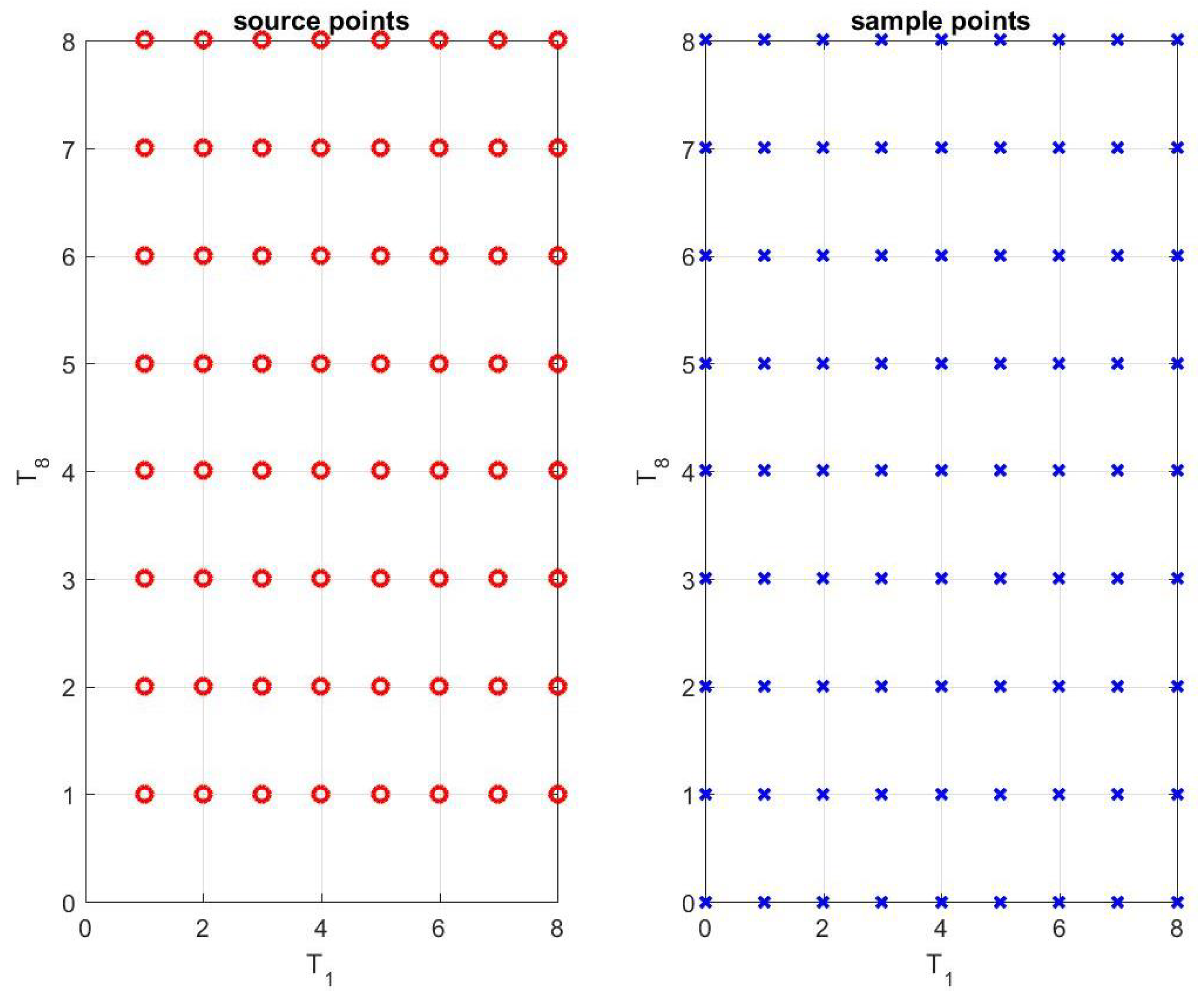
2.1. Radial Basis Function (RBF) Expansion

For fixed t and $\mathbf{x}$, R as a function of $T_1$ and $T_8$ is defined over the semi-infinite region ${\mathsf{\Omega }}_T=[0,\infty )\times [0,\infty )$. A RBF meshless approximation will be much more cost-effective than the regular finite difference discretization. To make the model biologically meaningful, homogeneous Dirichlet conditions are imposed over $\partial {\mathsf{\Omega }}_T$ which suggest the choice of radio basis functions in the form of

$${\varphi }_j\left(T\right)=e^{-\alpha \parallel T-T^j{\parallel }^2},\forall j=1,\cdots ,M_0.$$

They satisfy the far end boundary conditions automatically. Here we use $T=(T_1,T_8)$ and $T^j=(T_1^j,T_8^j)$ to represent points in the $T_1{T}_8$-plane. In particular, $T^j$, $\forall j=1,\cdots ,M_0$, are the $M_0$ source points used to define the $M_0$ radio basis functions. $\alpha >0$ is a scaling factor termed shape parameter that can be adjusted to enhance the numerical accuracy, which will become clear later. $\parallel ·\parallel$ stands for the Euclidean norm.

At each iteration step and fixed spatial location, the $T_1$ and $T_8$ dependence of R is denoted by

$$R\left(T\right)=\sum _{j=1}^{M_0}{q}_j{\varphi }_j\left(T\right)$$

where $q_j$, $\forall j=1,\cdots ,M_0$, are the coefficients of the RBF expansion to be determined.

Once the grid values of R have been calculated, we determine the coefficients via interpolations. Let $M_I$ be the number of interior sample points and $M-M_I$ be the number of boundary sample points. They are also termed collocation points. Fitting the values of R at the interior points ${\widehat{T}}^i\in (0,\infty )\times (0,\infty )$, $\forall i=1,\cdots ,M_I$ and the boundary points ${\widehat{T}}^i$ on the edges $T_1=0$ and $T_8=0$, $\forall i=M_I+1,\cdots ,M$, yields the following $M\times M_0$ linear system for the coefficients $q_j^{\prime }s$,

$$\left[\begin{array}{cccc}\hfill {\varphi }_1\left({\widehat{T}}^1\right)& \hfill {\varphi }_2\left({\widehat{T}}^1\right)& \hfill \cdots & \hfill {\varphi }_{M_0}\left({\widehat{T}}^1\right)\\ \hfill ⋮& \hfill ⋮& \hfill ⋮\\ \hfill {\varphi }_1\left({\widehat{T}}^{M_I}\right)& \hfill {\varphi }_2\left({\widehat{T}}^{M_I}\right)& \hfill \cdots & \hfill {\varphi }_{M_0}\left({\widehat{T}}^{M_I}\right)\\ \hfill {\varphi }_1\left({\widehat{T}}^{M_I+1}\right)& \hfill {\varphi }_2\left({\widehat{T}}^{M_I+1}\right)& \hfill \cdots & \hfill {\varphi }_{M_0}\left({\widehat{T}}^{M_I+1}\right)\\ \hfill ⋮& \hfill ⋮& \hfill ⋮\\ \hfill {\varphi }_1\left({\widehat{T}}^M\right)& \hfill {\varphi }_2\left({\widehat{T}}^M\right)& \hfill \cdots & \hfill {\varphi }_{M_0}\left({\widehat{T}}^M\right)\end{array}\right]\left[\begin{array}{c}\hfill q_1\\ \hfill ⋮\\ \hfill q_{M_0}\end{array}\right]=\left[\begin{array}{c}\hfill \overline{\mathbf{R}}\\ \hfill \mathbf{0}\end{array}\right]$$

(14)

where $\overline{\mathbf{R}}$ is an $M_I$ dimensional vector storing the numerical values of R at the $M_I$ interior sampling locations, and $\mathbf{0}$ is the $(M-M_I)$ dimensional zero vector reflecting the homogeneous Dirichlet conditions.

The coefficient matrix of the above linear system is dense but of a small scale. For $\alpha >0$ and $M=M_0$, it is positive-definite [42] with the Gaussian basis functions, which guarantees the uniqueness of the solution. Desired condition number of the coefficient matrix can also be achieved by properly adjusting the scaling factor $\alpha$, the source and collocation points, $T^j$ and ${\widehat{T}}^j$[42]. Least squares approximation can be used to solve the $M\times M_0$ linear system when $M>M_0$, which is preferred in this work.

2.2. Finite Difference WENO5 Discretization

The spatial divergence ${\nabla }_{\mathbf{x}}·\left(R\mathbf{K}\left(R\right)\right)$ is determined using WENO5 [39]. For simplification of notation in the following illustration, we temporarily drop the $c_1^u$ dependence and denote

$$R\mathbf{K}\left(R\right)=\left[\begin{array}{c}\hfill {\left(R\mathbf{K}\left(R\right)\right)}_1\\ \hfill {\left(R\mathbf{K}\left(R\right)\right)}_2\end{array}\right]\mathrm{by}F\left(R\right)=\left[\begin{array}{c}\hfill F_1\left(R\right)\\ \hfill F_2\left(R\right)\end{array}\right].$$

This is valid since R will be updated for fixed $c_1^u$ and $c_8^u$ in the numerical simulation.

Consider the spatial discretization for any fixed $(T_1,T_8)$. Once the numerical values of R are computed over a uniform 2D mesh in the spatial domain, the grid values of the nonlinear flux term $F\left(R\right)$ can be generated via the RBF approximation and a high-order numerical integration scheme such as Simpson’s rule. Then the 2D finite difference WENO5 reconstruction based on the grid values $F\left(R_{ij}\right)$ can be implemented to output the numerical fluxes ${\widehat{F}}_1\left(R_{i+\frac{1}{2},j}\right)$ and ${\widehat{F}}_2\left(R_{i,j+\frac{1}{2}}\right)$.

Let

$${\widehat{F}}_1^{\left(1\right)}\left(R_{i+\frac{1}{2},j}\right)=\frac{1}{3}{F}_1\left(R_{i-2,j}\right)-\frac{7}{6}{F}_1\left(R_{i-1,j}\right)+\frac{11}{6}{F}_1\left(R_{ij}\right),$$

$${\widehat{F}}_1^{\left(2\right)}\left(R_{i+\frac{1}{2},j}\right)=-\frac{1}{6}{F}_1\left(R_{i-1,j}\right)+\frac{5}{6}{F}_1\left(R_{ij}\right)+\frac{1}{3}{F}_1\left(R_{i+1,j}\right),$$

$${\widehat{F}}_1^{\left(3\right)}\left(R_{i+\frac{1}{2},j}\right)=\frac{1}{3}{F}_1\left(R_{ij}\right)+\frac{5}{6}{F}_1\left(R_{i+1,j}\right)-\frac{1}{6}{F}_1\left(R_{i+2,j}\right).$$

Define the smoothness indicators as

$${\beta }_1=\frac{13}{12}{\left(F_1\left(R_{i-2,j}\right)-2F_1\left(R_{i-1,j}\right)+F_1\left(R_{ij}\right)\right)}^2+\frac{1}{4}{\left(F_1\left(R_{i-2,j}\right)-4F_1\left(R_{i-1,j}\right)+3F_1\left(R_{ij}\right)\right)}^2,$$

$${\beta }_2=\frac{13}{12}{\left(F_1\left(R_{i-1,j}\right)-2F_1\left(R_{ij}\right)+F_1\left(R_{i+1,j}\right)\right)}^2+\frac{1}{4}{\left(F_1\left(R_{i-1,j}\right)-F_1\left(R_{i+1,j}\right)\right)}^2,$$

$${\beta }_3=\frac{13}{12}{\left(F_1\left(R_{ij}\right)-2F_1\left(R_{i+1,j}\right)+F_1\left(R_{i+2,j}\right)\right)}^2+\frac{1}{4}{\left(3F_1\left(R_{ij}\right)-4F_1\left(R_{i+1,j}\right)+F_1\left(R_{i+2,j}\right)\right)}^2.$$

The convex combination

$${\widehat{F}}_1\left(R_{i+\frac{1}{2},j}^{-}\right)={\omega }_1{\widehat{F}}_1^{\left(1\right)}\left(R_{i+\frac{1}{2},j}\right)+{\omega }_2{\widehat{F}}_1^{\left(2\right)}\left(R_{i+\frac{1}{2},j}\right)+{\omega }_3{\widehat{F}}_1^{\left(3\right)}\left(R_{i+\frac{1}{2},j}\right)$$

is applied to determine the numerical flux at the cell center. Here

$${\omega }_k=\frac{{\widehat{\omega }}_k}{{\widehat{\omega }}_1+{\widehat{\omega }}_2+{\widehat{\omega }}_3}\mathrm{with}{\widehat{\omega }}_k=\frac{{\gamma }_k}{{(ϵ+{\beta }_k)}^2},\mathrm{for}k=1,2,3.$$

The constants involved are set as

$${\gamma }_1=\frac{1}{10},{\gamma }_2=\frac{3}{5},{\gamma }_3=\frac{3}{10}\mathrm{and}ϵ={10}^{-6}.$$

Meanwhile ${\widehat{F}}_1\left(R_{i+\frac{1}{2},j}^{+}\right)$ can be determined in the same way using the right-biased cell with indices $i-1$, i, $i+1$, $i+2$ and $i+3$ instead. The numerical fluxes ${\widehat{F}}_2\left(R_{i,j+\frac{1}{2}}^{-}\right)$ and ${\widehat{F}}_2\left(R_{i,j+\frac{1}{2}}^{+}\right)$ can be determined via fixing i and varying j.

Finally the Lax–Friedrichs flux splitting

$$F_1\left(R_{i+\frac{1}{2},j}\right)=\frac{1}{2}\left({\widehat{F}}_1\left(R_{i+\frac{1}{2},j}^{-}\right)+{\widehat{F}}_1\left(R_{i+\frac{1}{2},j}^{+}\right)-{\alpha }_1\left(R_{i+\frac{1}{2},j}^{+}-R_{i+\frac{1}{2},j}^{-}\right)\right),$$

$$F_2\left(R_{i,j+\frac{1}{2}}\right)=\frac{1}{2}\left({\widehat{F}}_2\left(R_{i,j+\frac{1}{2}}^{-}\right)+{\widehat{F}}_2\left(R_{i,j+\frac{1}{2}}^{+}\right)-{\alpha }_2\left(R_{i,j+\frac{1}{2}}^{+}-R_{i,j+\frac{1}{2}}^{-}\right)\right)$$

is applied with

$${\alpha }_1=\underset{R}{max}|{\left(F_1\left(R\right)\right)}_R|,\mathrm{and}{\alpha }_2=\underset{R}{max}\left|{\left(F_2\left(R\right)\right)}_R\right|$$

to determine the spatial discretization of the nonlinear flux term

$${\nabla }_{\mathbf{x}}·F\left(R_{ij}\right)=\frac{F_1\left(R_{i+\frac{1}{2},j}\right)-F_1\left(R_{i-\frac{1}{2},j}\right)}{\mathsf{\Delta }x}+\frac{F_2\left(R_{i,j+\frac{1}{2}}\right)-F_2\left(R_{i,j-\frac{1}{2}}\right)}{\mathsf{\Delta }y}.$$

Please note that obtaining ${\alpha }_1$ and ${\alpha }_2$ analytically is quite complicated due to the integral form of the nonlinear flux term. Numerical approximation of them is sufficient to maintain the monotonicity.

2.3. Time Integration

We first introduce the following simplified notation for the full model.

$$\begin{array}{c}\hfill \frac{\partial R}{\partial t}=G_R(R,c_1^u,c_8^u)+d_R{\nabla }^{2}R\end{array}$$

(15)

$$\begin{array}{c}\hfill \frac{\partial c_1^u}{\partial t}=G_1(R,c_1^u,c_8^u)+d_{\mathrm{gal}}{\nabla }^2{c}_1^u\end{array}$$

(16)

$$\begin{array}{c}\hfill \frac{\partial c_8^u}{\partial t}=G_8(R,c_1^u,c_8^u)+d_{\mathrm{gal}}{\nabla }^2{c}_8^u\end{array}$$

(17)

2.3.1. Method of Integrating Factors

Using the method of integrating factors, the system of PDEs (15)–(17) are transformed into the following ODEs

$$\begin{array}{c}\hfill \frac{d\left(e^{-t{d}_R{\nabla }^2}R\right)}{dt}=e^{-t{d}_R{\nabla }^2}{G}_R(R,c_1^u,c_8^u)\end{array}$$

(18)

$$\begin{array}{c}\hfill \frac{d\left(e^{-t{d}_{\mathrm{gal}}{\nabla }^2}{c}_1^u\right)}{dt}=e^{-t{d}_{\mathrm{gal}}{\nabla }^2}{G}_1(R,c_1^u,c_8^u)\end{array}$$

(19)

$$\begin{array}{c}\hfill \frac{d\left(e^{-t{d}_{\mathrm{gal}}{\nabla }^2}{c}_8^u\right)}{dt}=e^{-t{d}_{\mathrm{gal}}{\nabla }^2}{G}_8(R,c_1^u,c_8^u)\end{array}$$

(20)

where $e^{-t\mu {\nabla }^2}$ denotes the operator exponential involving the diffusion operator with diffusivity $\mu$.

2.3.2. Time Integration Method

Equations (18)–(20) are all in the general form of

$$\frac{d\left(e^{-t\mu {\nabla }^2}u\right)}{dt}=e^{-t\mu {\nabla }^2}F\left(u\right)\mathrm{or}\frac{dY}{dt}=e^{-t\mu {\nabla }^2}F\left(e^{t\mu {\nabla }^2}Y\right)$$

which can be solved using various time integrators [43,44,45,46]. We use a third-order explicit Runge–Kutta method (SEIF3) [47].

Denote the numerical approximation of u at time step n by $U^n$ and the spatial discretization of $\mu {\nabla }^2$ by C. Then SEIF3 reads

$$\begin{array}{cc}\hfill & U^{\left(1\right)}=e^{\mathsf{\Delta }tC/2}\left(U^n+\frac{\mathsf{\Delta }t}{2}F\left(U^n\right)\right),\hfill \\ \hfill & U^{\left(2\right)}=e^{\mathsf{\Delta }tC}\left(U^n-\mathsf{\Delta }tF\left(U^n\right)\right)+2\mathsf{\Delta }t{e}^{\mathsf{\Delta }tC/2}F\left(U^{\left(1\right)}\right),\hfill \\ \hfill & U^{n+1}=e^{\mathsf{\Delta }tC}\left(U^n+\frac{\mathsf{\Delta }t}{6}F\left(U^n\right)\right)+\frac{2}{3}\mathsf{\Delta }t{e}^{\mathsf{\Delta }tC/2}F\left(U^{\left(1\right)}\right)+\frac{\mathsf{\Delta }t}{6}F\left(U^{\left(2\right)}\right).\hfill \end{array}$$

With periodic boundary conditions on $\partial \mathsf{\Omega }$, the evaluation of $e^{\beta \mathsf{\Delta }tC}U$ for any matrix $\beta \mathsf{\Delta }tC$ can be achieved using FFT. In case of non-periodic boundary conditions, variations of the presented IF coupled with FFT can be applied, such as compact integration methods via Krylov subspace approximations [43,44,45,46]. The main idea is to approximate the resulting vector $e^{\beta \mathsf{\Delta }tC}U$ by a vector in the span of some properly chosen basis that depends on the matrix C and imposed boundary conditions. The FFT approach based on Fourier series presented here can be viewed as a special case of the general Krylov expansion.

2.4. Numerical Algorithm and Complexity

The detailed numerical algorithm is provided as follows.

• Let $M_0$ be the number of source points in the $T_1{T}_8$-plane. Initialize $M_0$ different R’s over a 2D spatial mesh of $N\times N$ grids, associated with the source points.
• Initialize $c_1^u$ and $c_8^u$ over the same 2D spatial mesh of $N\times N$ grids.
• Compute exactly the partial derivatives and integrals of radio basis functions to be used later, including

  $$\frac{\partial {\varphi }_j}{\partial T_1},\frac{\partial {\varphi }_j}{\partial T_8},{\int }_0^{\infty }{\int }_0^{\infty }{\varphi }_{j}d{T}_{1}d{T}_8,$$

  $${\int }_0^{\infty }{\int }_0^{\infty }{T}_1{\varphi }_{j}d{T}_{1}d{T}_8,{\int }_0^{\infty }{\int }_0^{\infty }{T}_8{\varphi }_{j}d{T}_{1}d{T}_8,\forall j=1,\cdots ,M_0.$$
• Perform the following at each time step up to the desired $t=T$.
  • Determine the coefficients $q_j$’s in the RBF expansion for all the R’s.
  • Compute $G_R(R,c_1^u,c_8^u)$ using WENO5 finite difference discretization.
  • Update R explicitly using SEIF3.
  • Determine $G_1(R,c_1^u,c_8^u)$ and $G_8(R,c_1^u,c_8^u)$ via linear combinations of the known information from the radio basis functions.
  • Update $c_1^u$ and $c_8^u$ explicitly using SEIF3.

Steps 1 and 3 are most expensive. Step 1 requires solving $N^2$ linear systems of size $M\times M_0$ ($M\ge M_0$) via least squares with QR factorization. The complexity is $O(M_0^3+N^2{M}_0^2)$. For each $(T_1,T_8)$ block in Step 3, the worst-case complexity of FFT is $O(N^{2}lnN)$, hence the total complexity is $O(M_0{N}^{2}lnN)$ for $N\gg M_0$. The efficiency of the RBF meshless approach is due to its rapid convergence which requires rather small value of $M_0$.

3. Numerical Results

In this section, we present some numerical results for both the reduced and full systems. The biological parameters are as shown in Table 5. (See also references [17,48].) In all the following simulation, the spatial domain is set to be $\mathsf{\Omega }=[0,1]\times [0,1]$ so the rectangular spatial meshing is a routine process. Nevertheless the domain of computation is not confined to rectangles. For example, a circular region can be transformed into a rectangular one in polar coordinates hence all the numerical discretizations will still be valid with a change of variables. In case of general irregular domains, finite element WENO or the recently developed RBF-WENO can be applied instead of the finite difference WENO used in our work. This is one of our follow-up works in process.

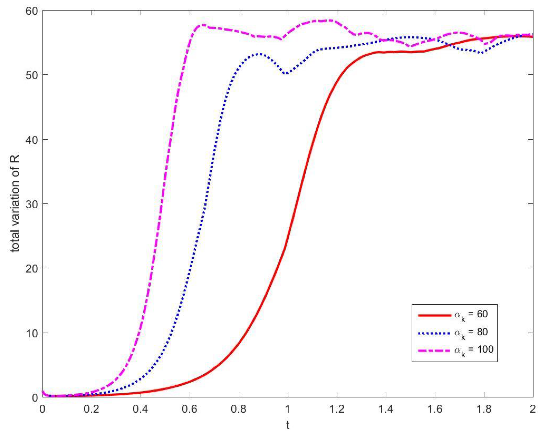
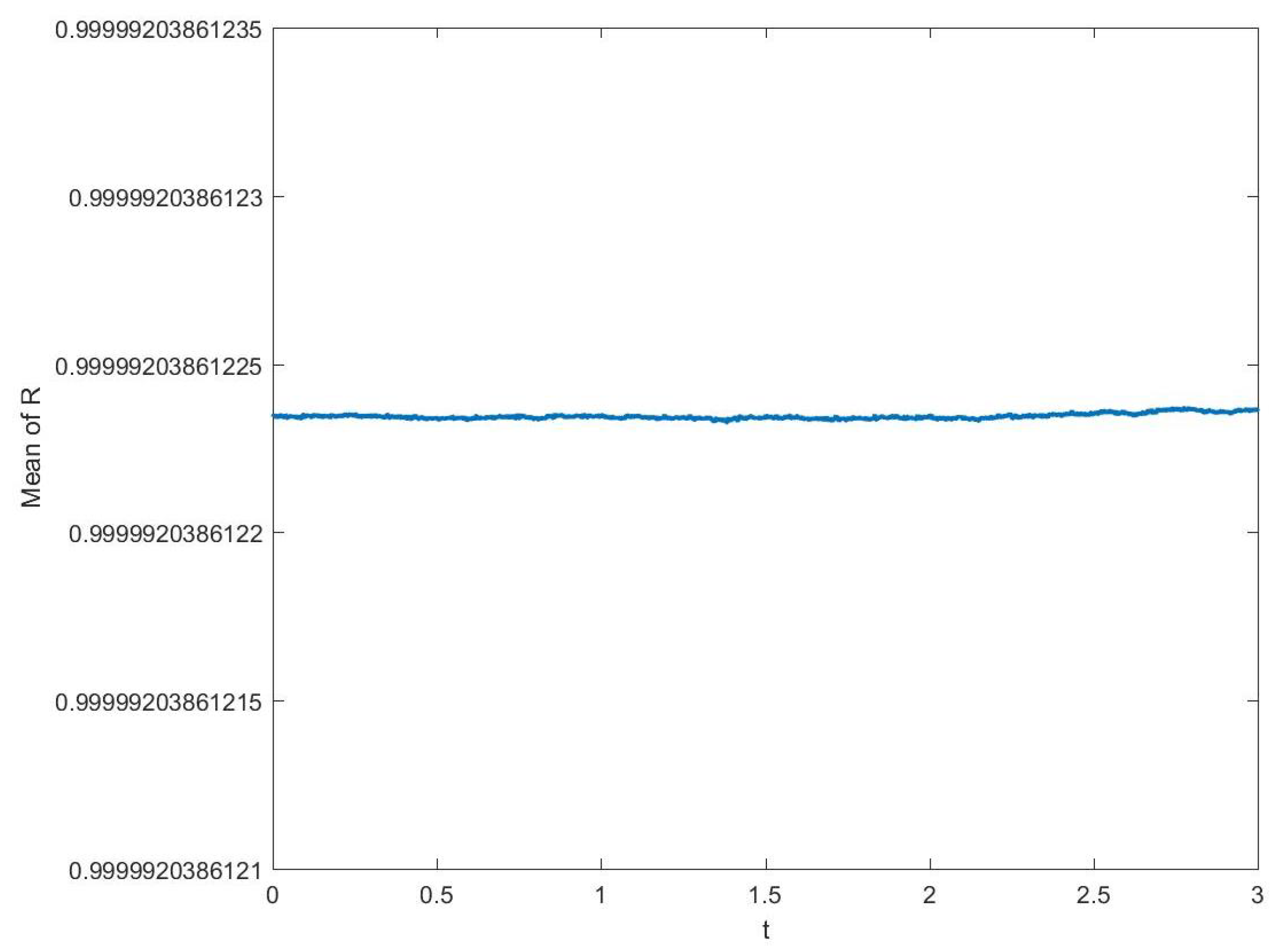
3.1. Convergence and Stability of Numerical Methods

3.1.1. Stability of Time Integration Method

The reduced model is solved to confirm the stability of the proposed time integration method coupled with WENO5 spatial discretization.

Since $c_1^u$ and $c_8^u$ diffuse much more rapidly than R within the time scale of simulation, explicit time iteration for the reaction terms is sufficient to capture the mild changes of them without stringent time stepping restrictions. Initialize R, $c_1^u$ and $c_8^u$ close to their spatially constant steady states. Set the uniform spatial grids with mesh size ${\displaystyle \mathsf{\Delta }x=\frac{1}{2^7}}$. Time step $\mathsf{\Delta }t=0.3\mathsf{\Delta }x$ guarantees the stability of SEIF3 for ${\tilde{\alpha }}_K=60$, 80 and 100, as shown in Figure 3 where the time evolutions of the total variation (TV) of R for these parameter choices are plotted. Denote the $ij$-th spatial grid by $(x_i,y_j)$. The total variation is computed numerically via

$$\mathrm{TV}\left(R\right)=\sum _j|R_x\left(y_{j+1}\right)-R_x\left(y_j\right)|\mathrm{where}{R}_x\left(y_j\right)=\sum _i|R(x_{i+1},y_j)-R(x_i,y_j)|.$$

Starting from the beginning, TV of R increases rapidly due to the dominance of cell-cell adhesion over diffusion, which leads to the gradual formation of patterns until TV reaches a peak. Then the adhesive force is well balanced by the diffusion and TV maintains afterwards except for the slight fluctuations due to the shape adjustment of patterns at the final stage. Clearly pattern formation occurs more rapidly with higher ${\tilde{\alpha }}_K$ to which more detailed biological explanation will be provided in Section 3.4. The conservation of spatial mean of R throughout the time iteration can also be confirmed by our computation. As an example, the evolution of spatial mean of R with ${\tilde{\alpha }}_K=60$ is shown in Figure 4.

3.1.2. Convergence of RBF Approximation

Recall that $R(t,\mathbf{x},T1,T8)$ is governed by an advection equation with homogeneous Dirichlet boundary conditions at each fixed spatial location $\mathbf{x}$; see (1). To study the dynamics of R in $T_1{T}_8$-space, let us temporarily drop $\mathbf{x}$. Advection in $T_1{T}_8$-space is determined by the velocity field $(\tilde{\gamma }(c_1^u,c_8^u,T_1),\tilde{\delta }(c_8^u,T_8))$ given in (6) and (7), respectively. Keeping $\mathbf{x}$ and $c_1^u(t,\mathbf{x}),c_8^u(t,\mathbf{x})$ fixed, let us write $\tilde{\gamma }(c_1^u,c_8^u,T_1)=\gamma \left(T_1\right)$ and $\tilde{\delta }(c_8^u,T_8)=\delta \left(T_8\right)$. A plot of the velocity field $(\gamma ,\delta )$ in the $T_1{T}_8$-plane is given in Figure 5. There is a unique zero $({\overline{T}}_1,{\overline{T}}_8)$ with ${\overline{T}}_1,{\overline{T}}_8>0$, and every flow line with positive initial $T_1$ converges to $({\overline{T}}_1,{\overline{T}}_8)$. This means that R is advected towards this zero and, again fixing the position $\mathbf{x}$ and the concentrations $c_1^u(t,\mathbf{x}),c_8^u(t,\mathbf{x})$, R becomes concentrated at $({\overline{T}}_1,{\overline{T}}_8)$. In fact, under simplifying assumptions, it is possible to show that $R(t,T_1,T_8)$ converges to a Dirac delta distribution centered at $({\overline{T}}_1,{\overline{T}}_8)$ [17]. This is the assumption in the case of fast counterreceptor dynamics (i.e., fast dynamics in $T_1{T}_8$-space), which yields the reduced model (10)–(12). Thus, the full model is relevant for the case that the flux term in $T_1$ and $T_8$ takes on values for which the variance of the distribution $R(t,T_1,T_8)$ is large enough that it cannot be reasonably approximated by a delta-distribution, i.e., that the decay from the peak is not too rapid to lose the smoothness of $R(t,T_1,T_8)$. On the other hand, the decay is rapid enough so that the support of $R(t,T_1,T_8)$ can be approximated by a compact computational region, which is set as $\left[0.8\right]\times [0,8]$ in our numerical simulation.

At each fixed spatial location $\mathbf{x}$, we initialize R with an Gaussian distribution

$$R(0,T_1,T_8)=e^{-{\alpha }_0{\parallel T-T^0\parallel }^2}.$$

This assumption of a joint Gaussian distribution for the membrane-bound counterreceptor densities $T_1$ and $T_8$ is biologically plausible. Indeed, since the density of counterreceptors on an individual cell may be modeled as the cumulative outcome of many, partly uncorrelated small-scale events, an overall normal distribution is a reasonable assumption by an appeal to the central limit theorem; this standard argument is well laid out in e.g., [49]. Empirical data supports this normality assumption, see, e.g., Figure 5 in [50] showing the distribution of PTK7 receptor density for human HeLa cells. The above heuristic arguments mean that a series of deformed Gaussian distributions centered at various $(T_1,T_8)$ locations, $R(t,T_1,T_8)$, will be generated through the advection process and then determined via a RBF approximation. That is $R(t,T_1,T_8)$ will be written as a linear combination of the Gaussian basis ${\varphi }_j$ introduced in Section 2.1 for $t>0$.

The accuracy of the RBF approximation to $R(t,T_1,T_8)$ depends on the variance and center location of $R(t,T_1,T_8)$, the source and sample points as well as the shape parameter $\alpha$ in the Gaussian basis. Recall that the source points are the data points used to define the RBFs and the sample points are the data points used for interpolation. They are set to be the lattice grids as shown in Figure 6 to fit the rectangular domain of computation. To properly choose the shape parameter $\alpha$, we shall study the effectiveness of the RBF approximation to various Gaussian functions since they behave similarly as $R(t,T_1,T_8)$ based on the above discussions. Here are the constructive observations from numerical simulation.

• Decreasing $\alpha$ flattens the Gaussian basis functions but significantly increases the condition number of the coefficient matrix in the linear system (14), some examples are given in

  Table 2. Condition numbers of the coefficient matrix generated by the Gaussian basis approximation with various shape parameters $\alpha$.

  $\alpha$	1	$\sqrt{2}$	$\sqrt{3}$	2	$\sqrt{5}$
  cond(A)	$12605242.6168$	$119581.1562$	$12897.4244$	$3268.6161$	$1258.3852$
  $\alpha$	$\sqrt{6}$	$\sqrt{7}$	$\sqrt{8}$	3	$\sqrt{10}$
  cond(A)	$616.6931$	$352.5934$	$224.0349$	$153.5909$	$111.4601$

  .
• A Gaussian function with shape parameter ${\alpha }_0$ is more accurately approximated by the Gaussian basis functions with shape parameter $\alpha$ closest to ${\alpha }_0$, as shown in

  Table 3. RBF approximation errors in interpolating different Gaussian functions with shape parameters ${\alpha }_0=1,\sqrt{10}$ and $\sqrt{60}$ using Gaussian basis functions with shape parameters $\alpha =1,2,\cdots ,10$, all centered at $(4.5,4.5)$. The error is defined as the absolute difference between the mean values of the original Gaussian function and its RBF approximation. Regardless of ${\alpha }_0$, the error is minimized when $\alpha$ is closest to ${\alpha }_0$. In the left most column, the minimum error is of smallest scale when the flattest Gaussian function among the three is approximated. However it is most sensitive to the change of $\alpha$ due to the ill-conditioning of the coefficient matrix.

  $\alpha$	${\alpha }_0=1$	${\alpha }_0=\sqrt{10}$	${\alpha }_0=\sqrt{60}$
  1	$4.5066\times {10}^{-12}$	$5.8372\times {10}^{-1}$	$2.6456\times {10}^0$
  2	$6.9270\times {10}^{-5}$	$8.6883\times {10}^{-3}$	$4.7110\times {10}^{-2}$
  3	$2.4228\times {10}^{-5}$	$1.4438\times {10}^{-4}$	$1.3279\times {10}^{-2}$
  4	$6.4800\times {10}^{-4}$	$2.9978\times {10}^{-4}$	$1.0304\times {10}^{-2}$
  5	$4.6742\times {10}^{-3}$	$1.5031\times {10}^{-3}$	$9.4189\times {10}^{-3}$
  6	$1.7373\times {10}^{-2}$	$5.4889\times {10}^{-3}$	$7.6930\times {10}^{-3}$
  7	$4.4186\times {10}^{-2}$	$1.3959\times {10}^{-2}$	$4.1405\times {10}^{-3}$
  8	$8.8846\times {10}^{-2}$	$2.7960\times {10}^{-2}$	$1.7169\times {10}^{-3}$
  9	$1.5073\times {10}^{-1}$	$4.7651\times {10}^{-2}$	$9.9534\times {10}^{-3}$
  10	$2.2914\times {10}^{-1}$	$7.2446\times {10}^{-2}$	$2.0325\times {10}^{-2}$

  .
• The Gaussian basis approximation to a flatter Gaussian function achieves higher order of accuracy with matching Gaussian basis functions (i.e., with $\alpha$ closest to ${\alpha }_0$), as shown in Table 3.
• A Gaussian function centered close to the boundary is less accurately approximated by any Gaussian basis, as shown in

  Table 4. RBF approximation errors in interpolating different Gaussian functions with shape parameters ${\alpha }_0=1,2,3$ and 4 and centered at integer locations $(k,k)$, for $1\le k\le 8$, using Gaussian basis functions with shape parameters $\alpha =\sqrt{10}$. The error is defined as the absolute difference between the mean values of the original Gaussian function and its RBF approximation. Regardless of ${\alpha }_0$, larger approximation error is observed when interpolating a Gaussian function centered close to the boundary.

  Center of Gaussian	${\alpha }_0=1$	${\alpha }_0=2$	${\alpha }_0=3$	${\alpha }_0=4$
  $(1,1)$	$9.9574\times {10}^{-2}$	$4.8791\times {10}^{-2}$	$2.1756\times {10}^{-2}$	$1.3630\times {10}^{-2}$
  $(2,2)$	$4.7393\times {10}^{-3}$	$1.1759\times {10}^{-4}$	$1.1658\times {10}^{-4}$	$8.5660\times {10}^{-4}$
  $(3,3)$	$4.7065\times {10}^{-5}$	$3.0244\times {10}^{-5}$	$1.5277\times {10}^{-5}$	$4.8755\times {10}^{-6}$
  $(4,4)$	$1.5090\times {10}^{-5}$	$4.1839\times {10}^{-5}$	$2.0807\times {10}^{-5}$	$3.0175\times {10}^{-4}$
  $(5,5)$	$1.4583\times {10}^{-5}$	$1.9582\times {10}^{-4}$	$9.7912\times {10}^{-5}$	$9.3613\times {10}^{-4}$
  $(6,6)$	$5.8444\times {10}^{-5}$	$9.0433\times {10}^{-4}$	$4.5325\times {10}^{-4}$	$3.8596\times {10}^{-3}$
  $(7,7)$	$1.7513\times {10}^{-2}$	$4.4026\times {10}^{-3}$	$2.2741\times {10}^{-3}$	$1.8559\times {10}^{-2}$
  $(8,8)$	$4.1557\times {10}^{-1}$	$2.1837\times {10}^{-1}$	$3.0318\times {10}^{-2}$	$1.5591\times {10}^{-1}$

  . This effect is most obvious for the flattest Gaussian function (left most column in Table 4) since it does not decay fast enough to smoothly match the homogeneous Dirichlet condition at boundaries $T_1=0$ and $T_8=0$. When the variance of a Gaussian function decreases, it decays fast enough so that the boundary disagreement is negligible compared to the interpolating error caused by the non-flatness of the Gaussian function. This explains why the minimum error does not have to occur exactly at the center of $[0.8]\times [0,8]$, referring to the right most column in Table 4.

Numerical results of $R(t,T_1,T_8)$ will be provided in Section 3.4 in which we can observe that the mean peak location of $R(t,T_1,T_8)$ stays reasonably away from the boundaries. As a result, setting $\alpha =\sqrt{10}$ in all the numerical simulation yields desired conditioning and approximation accuracy.

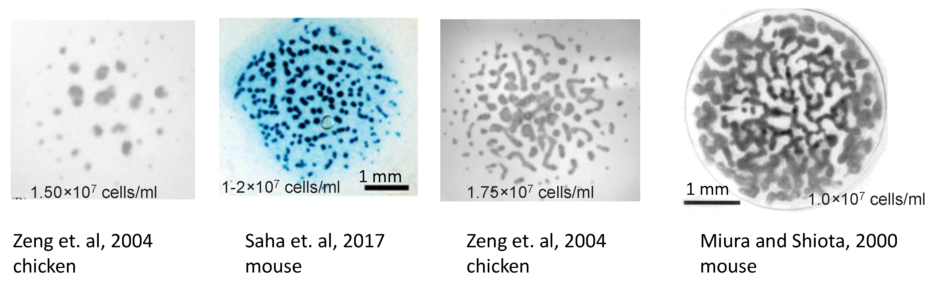
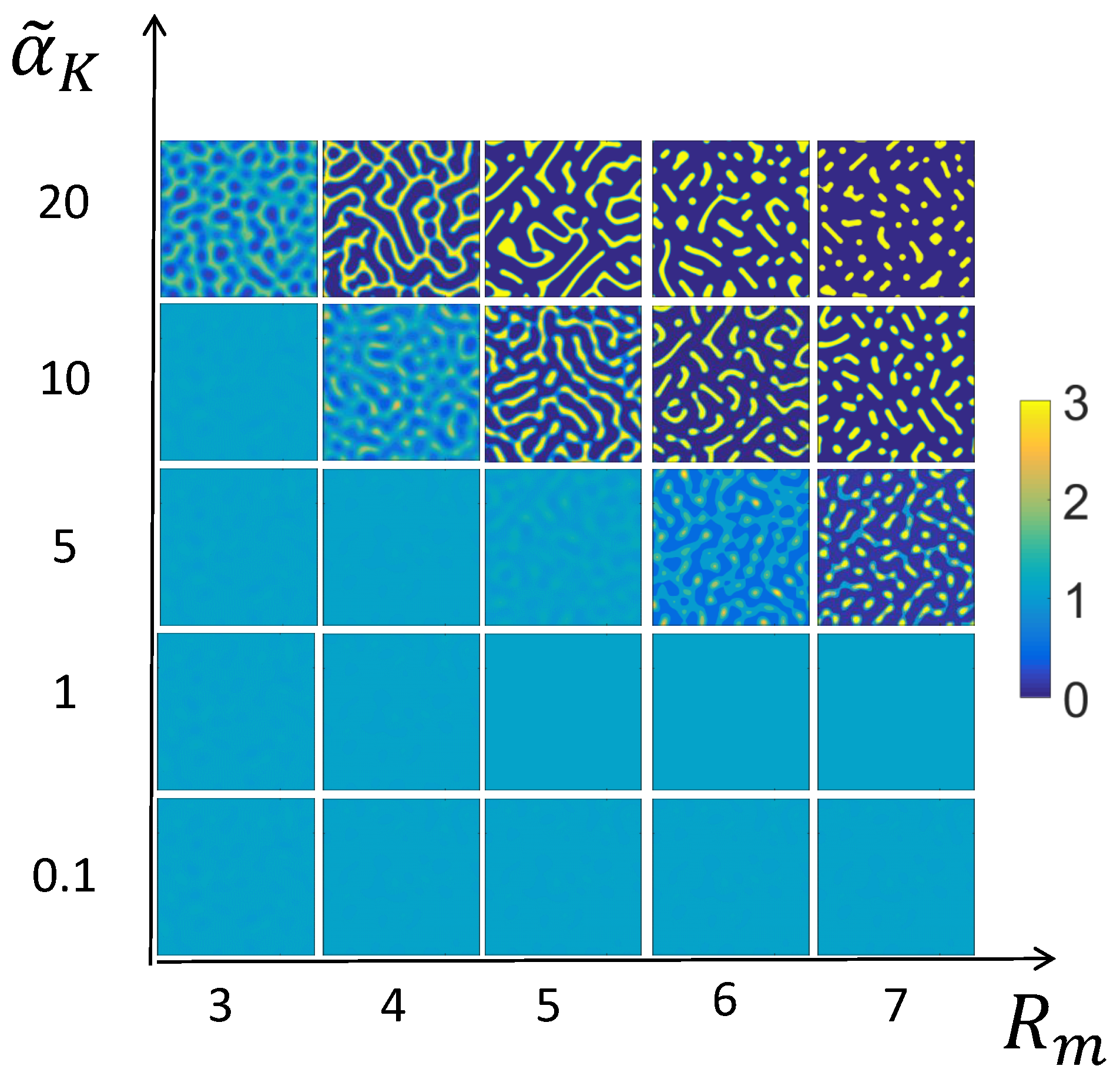
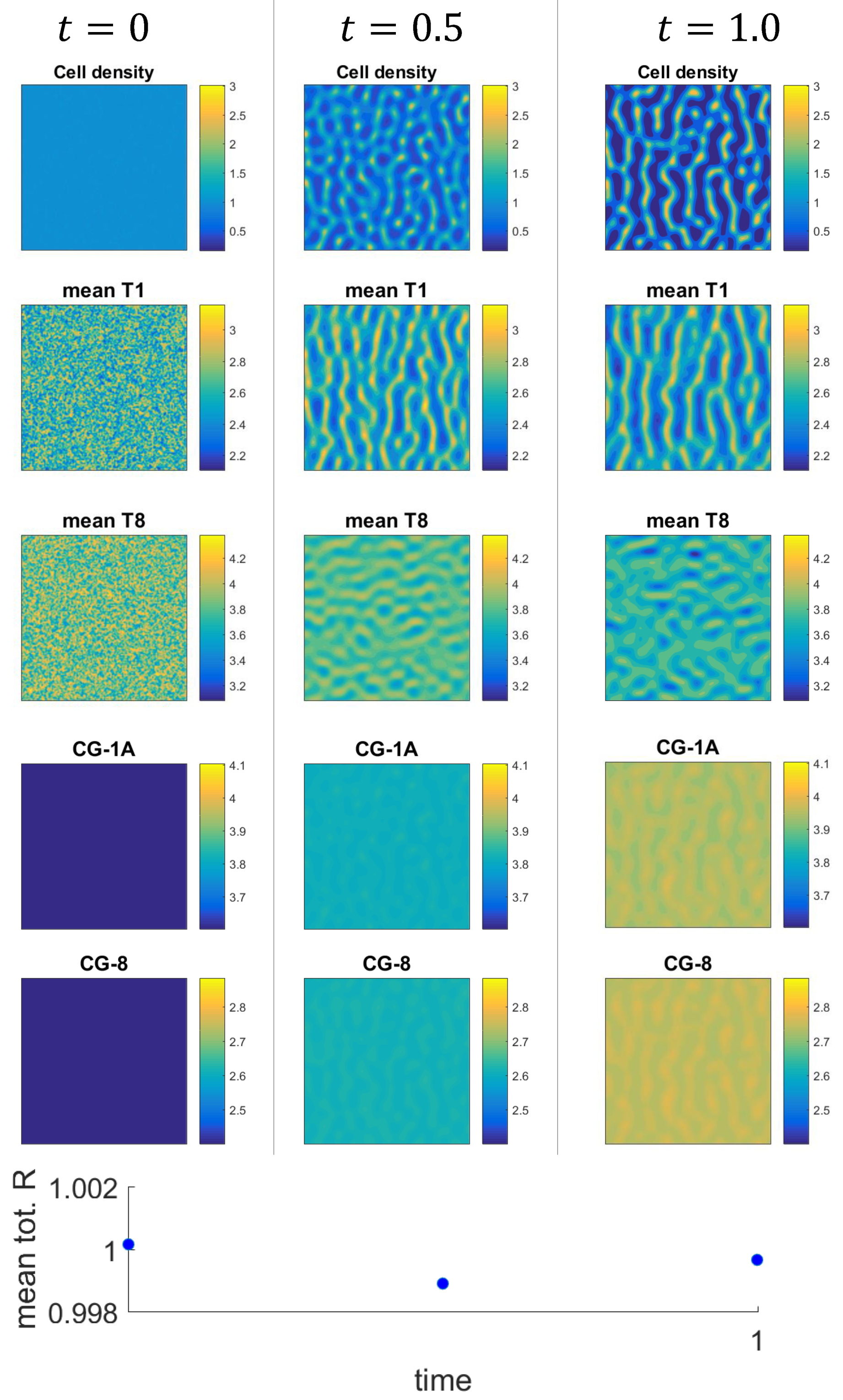
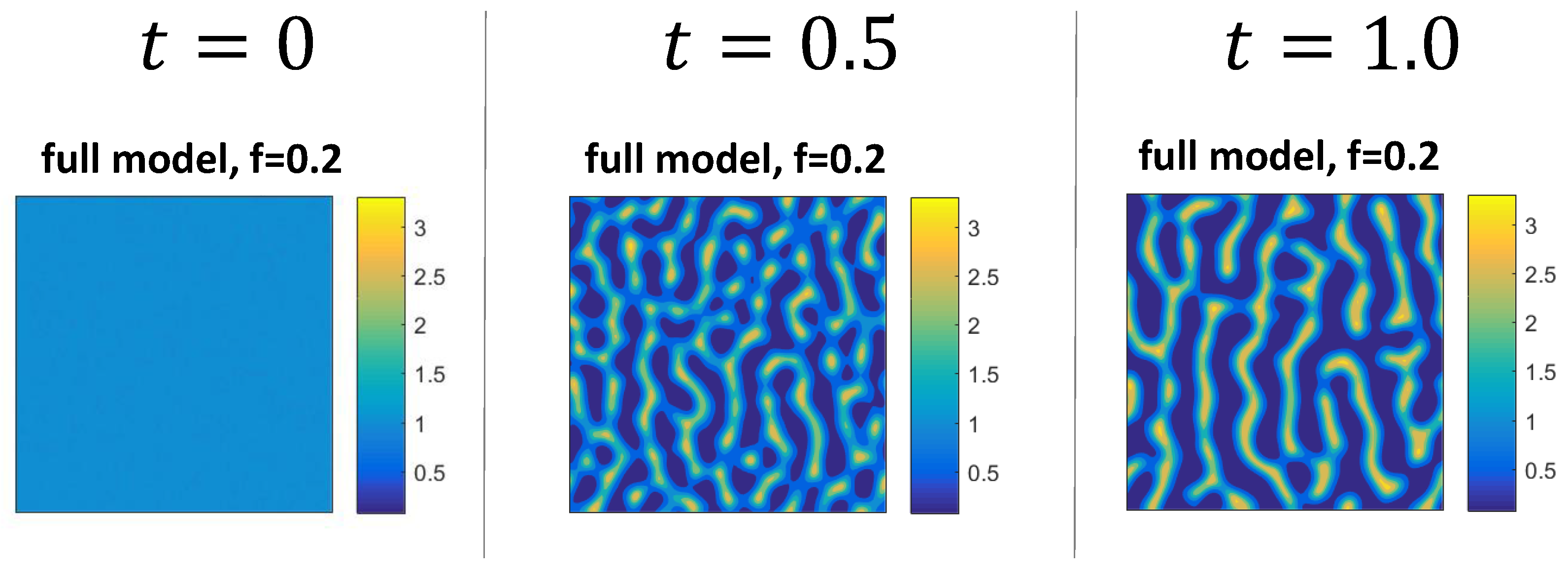
3.2. Numerical Examples for the Full System

Starting from initial conditions close to a spatially constant distribution of the cell density, the system forms characteristic stripe-like or labyrinthine patterns similar to patterns observed in cultures of embryonic chick mesenchymal cells in vitro; see Figure 1 for photos of corresponding experimentally obtained patterns.

Figure 7 illustrates the process of pattern formation in the full model (1)–(3) as labyrinthine patterns in the total cell density emerge. These patterns are quasi steady state patterns in the sense that after their rapid establishment, they change little over long time scales. Please note that the overall concentrations of CG-1A and CG-8, $c_1^u$ and $c_8^u$, are increasing throughout the simulation. This is in accordance with experiments [17,34].

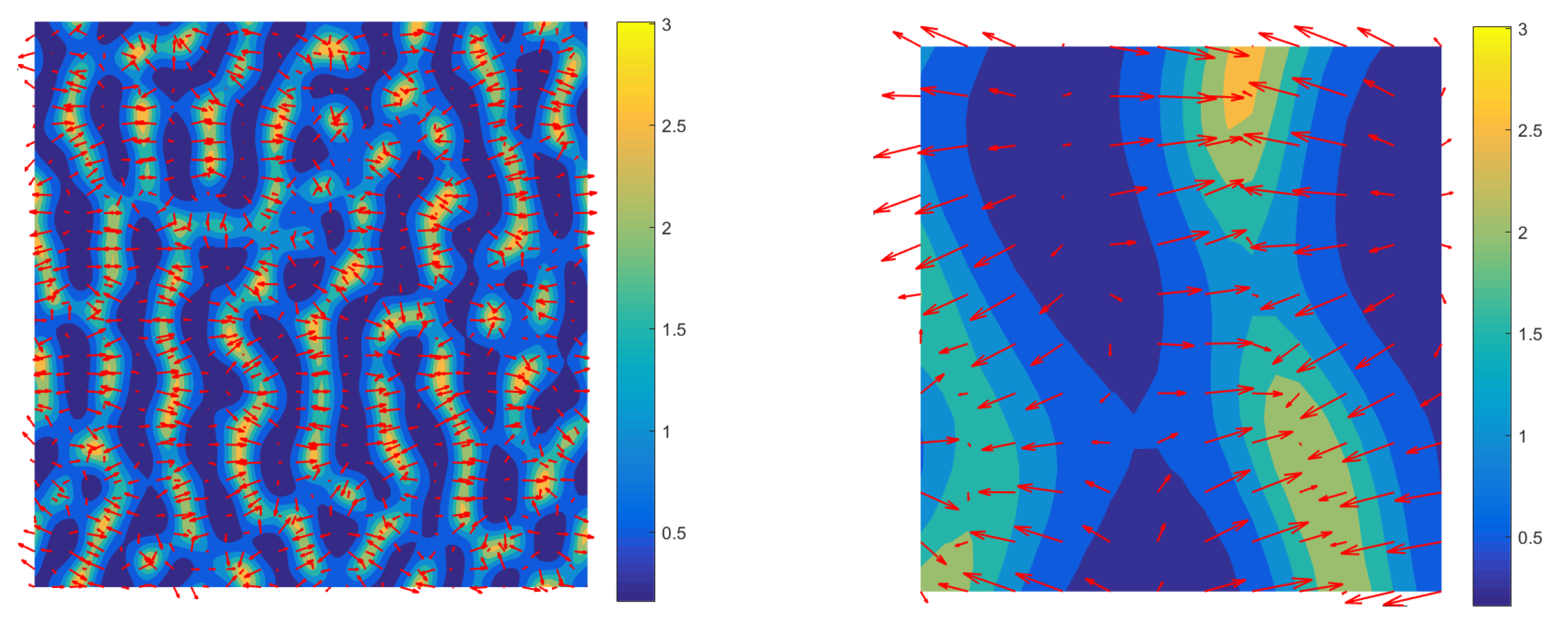
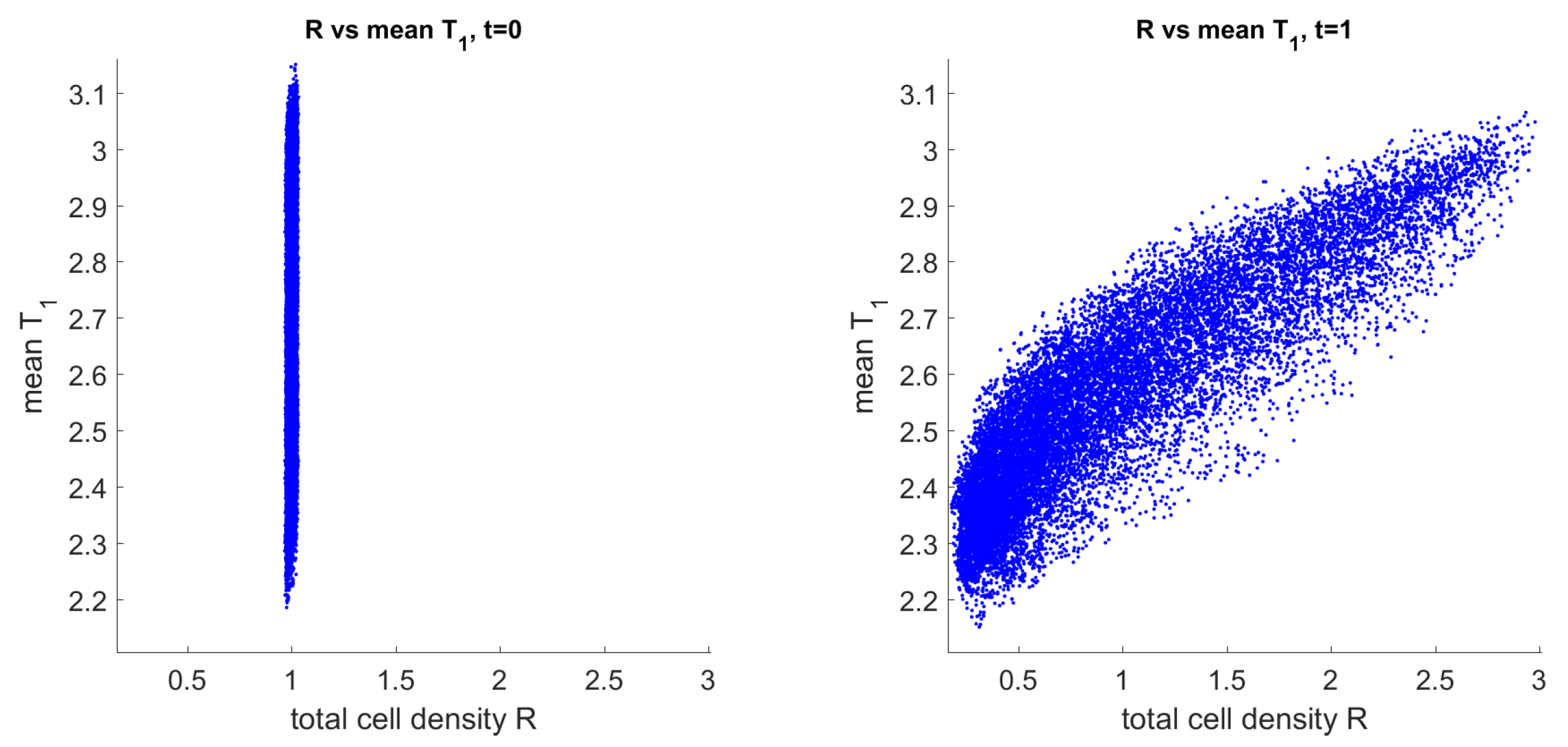
3.3. Mechanism of Pattern Formation

The term responsible for the formation of patterns in the total cell density ${\int }_0^{\infty }{\int }_0^{\infty }R(t,x,y,T_1,T_8)d{T}_{1}d{T}_8$ is the cell-cell adhesion term $\mathbf{K}\left(R\right)$ in (8). This term describes an effective motion up the gradients of the cell density R, but modulated by the CR-1 counterreceptor density $T_1$, so that the larger $T_1$, the larger the flux. This flux is balanced by the diffusive flux in the quasi steady state. An illustration of the adhesive flux is given in Figure 8.

Because the cell adhesion flux term $\mathbf{K}\left(R\right)$ increases with counterreceptor density $T_1$, the cell aggregations (areas of high cell density) are primarily made up of cells with large density $T_1$. This can be seen in the plots of the mean of $T_1$ in Figure 7. Regions of larger mean $T_1$ also correspond to regions of higher total cell density. This observation is confirmed when plotting the cell density against the mean counterrecptor density $T_1$ in Figure 9. Initially (time $t=0$), there is no relation between these two variables since the cells are assumed to be completely mixed in the initial data. At the end of the simulation ($t=1.0$), there is a clear correlation between cell density and mean $T_1$.

The counterreceptor $CR-1$ not only mediates cell-cell adhesion, but it is also indirectly involved in the production of CG-1A, so that this numerical result is consistent with the experimental finding that production of CG-1A is elevated inside condensations [17,34].

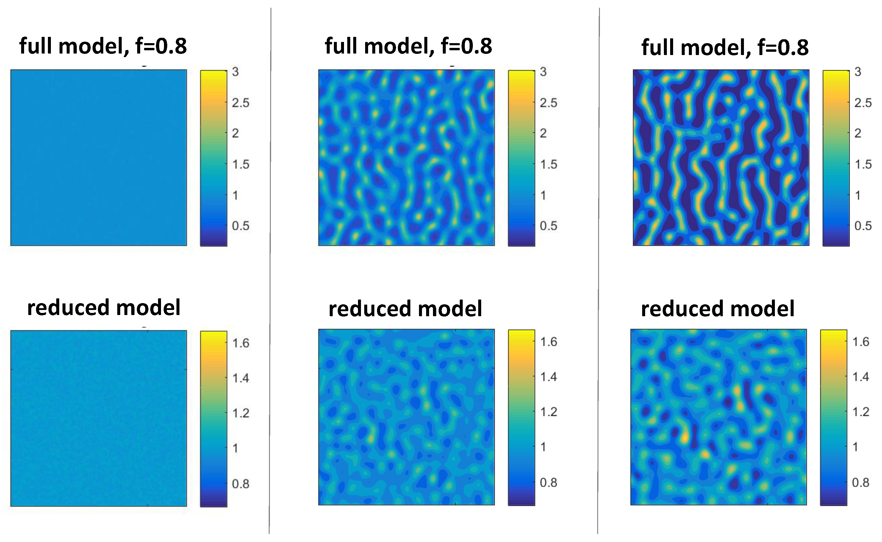
3.4. Comparison of Solutions to the Full and Reduced Models

Since the cell density $R(t,\mathbf{x})$ in the reduced system (10)–(12) does not depend on the counterreceptor densities $T_1$ and $T_8$, the related simulation is only two-dimensional compared to the effectively four-dimensional full system. This is certainly a computational advantage over the full system (1)–(3). However, its derivation rests on the additional modeling hypothesis that production of counterreceptors happens on a faster time scale than production of galectins, an assumption whose validity is unknown and indeed difficult to test experimentally [17]. While the system still produces patterns in the cell densities, and thus can be seen as a simple, but useful model of chondrogenesis, there are certain aspects of the full model that are lost. For instance, the parameter f describes the affinity of CG-8 to bind to the counterreceptor CR-1 relative to the counterreceptor CR-8 and thus is vital to an understanding of the role of CG-8. By binding to CR-1, CG-8 is effectively in competition with CG-1A; thus f describes the ’competitiveness’ of CG-8. In the reduced model, f does not appear because in the steady-state assumption of fast equilibration of CR-1, the density $c_1$ of the complex of CG-1A and CR-1 is independent of f. Thus, the reduced model is inadequate to investigate the subtle role of CG-8. As an illustration, we show some numerical results in Figure 10. All three simulations are corresponding to the same parameter set, with the exception of the parameter f. In the case of $f=0.8$, or high competitiveness of CG-8, a clear pattern in the total cell density emerges. Areas of high cell density also correspond to areas of high average density of CR-1 (see Figure 7, column 2). In other words, the condensations are formed by cells with higher average CR-1 densities on their membranes. In the case of $f=0.2$, or ‘low’ competitiveness of CG-8, the cell pattern is even more pronounced with very clear boundaries between high and low cell densities. This is because cell-cell adhesion is mediated by the complex of CG-1A and CR-1, which is now less affected by the competition of CG-8, leading to stronger cell-cell adhesion. Finally, in the reduced model, the dependency on the parameter f is lost through the steady-state assumption for CR-1. Now all cells have essentially the same density of CR-1. The pattern is much fainter, pointing to the crucial effect of different densities of CR-1, i.e., the dependence of the cell density on the variable $T_1$. These examples illustrate that the full model enables a much more in-depth analysis of the interplay of CG-1A and CG-8 and its significance for the formation of condensations.

4. Conclusions and Future Investigations

We present a RBF meshless approximation coupled with the mesh-based finite difference discretization to relax the computational complexity caused by the high dimensionality in a nonlinear advection-reaction-diffusion system. The span of rather small sets of Gaussian basis functions can provide desired accuracy in the numerical approximation of the structure variable dependence of the cell condensation to be captured. This high efficiency of the meshfree approach significantly reduces the computational cost of a 4-dimensional system to one that is comparable to a 2-dimensional system. We presented some sample simulations that illustrate how this system gives rise to spatial patterns in the cell density resembling in vitro condensations. Additional insights into the mechanism of pattern formation can be gained by investigating not only the final pattern, but also the temporal development of the process, and also by simulating specific experiments [34,48]. We will present these results in a separate forthcoming publication.

The RBF meshfree approximation not only couples well with the finite difference spatial discretization presented in this work, but also will fit in other types of spatial discretization, such as finite element or finite volume methods, depending on the properties of spatial domain as well as the prescribed boundary conditions. Furthermore, a complete meshfree scheme in both structural and spatial domains will be one of our future attempts, allowing applications to extensions of the chondrogenesis model at hand as well as other biological models. This is especially relevant for modeling in vivo chondrogenesis, which takes place within the growing limb bud, thus necessitating growing domains with curved boundaries [51,52].

Another numerical extension of this work is to optimize the RBF approximation error through the development of adaptivity strategies for RBFs via dynamically adjusting the source points, the sample points and the shape parameters. This will allow cost-effective meshfree approximations of non-smooth or rapidly changing biological quantities involved in various complex dynamical systems.

References

1. Forgacs, G.; Newman, S. Biological Physics of the Developing Embryo; Cambridge University Press: Cambridge, UK, 2005. [Google Scholar]
2. Wolpert, L.; Tickle, C.; Arias, A.M. Principles of Development; Oxford University Press: Oxford, UK, 2015. [Google Scholar]
3. Rejniak, K.A.; McCawley, L.J. Current trends in mathematical modeling of tumor–microenvironment interactions: A survey of tools and applications. Exp. Biol. Med. 2010, 235, 411–423. [Google Scholar] [CrossRef] [PubMed]
4. Altrock, P.M.; Liu, L.L.; Michor, F. The mathematics of cancer: Integrating quantitative models. Nat. Rev. Cancer 2015, 15, 730–745. [Google Scholar] [CrossRef] [PubMed]
5. Armstrong, N.J.; Painter, K.J.; Sherratt, J.A. A continuum approach to modelling cell-cell adhesion. J. Theor. Biol. 2006, 243, 98–113. [Google Scholar] [CrossRef] [PubMed] [Green Version]
6. Anguige, K.; Schmeiser, C. A one-dimensional model of cell diffusion and aggregation, incorporating volume filling and cell-to-cell adhesion. J. Math. Biol. 2008, 58, 395–427. [Google Scholar] [CrossRef]
7. Murakawa, H.; Togashi, H. Continuous models for cell-cell adhesion. J. Theor. Biol. 2015, 374, 1–12. [Google Scholar] [CrossRef] [Green Version]
8. Buttenschön, A.; Hillen, T.; Gerisch, A.; Painter, K.J. A space-jump derivation for non-local models of cell–cell adhesion and non-local chemotaxis. J. Math. Biol. 2018, 76, 429–456. [Google Scholar] [CrossRef]
9. Gerisch, A.; Chaplain, M.A.J. Mathematical modelling of cancer cell invasion of tissue: Local and non-local models and the effect of adhesion. J. Theor. Biol. 2008, 250, 684–704. [Google Scholar] [CrossRef]
10. Engwer, C.; Stinner, C.; Surulescu, C. On a structured multiscale model for acid-mediated tumor invasion: The effects of adhesion and proliferation. Math. Models Methods Appl. Sci. 2017, 27, 1355–1390. [Google Scholar] [CrossRef]
11. Painter, K.J.; Armstrong, N.J.; Sherratt, J.A. The impact of adhesion on cellular invasion processes in cancer and development. J. Theor. Biol. 2010, 264, 1057–1067. [Google Scholar] [CrossRef] [Green Version]
12. Chaplain, M.a.J.; Lachowicz, M.; Szymańska, Z.; Wrzosek, D. Mathematical modelling of cancer invasion: The importance of cell–cell adhesion and cell–matrix adhesion. Math. Models Methods Appl. Sci. 2011, 21, 719–743. [Google Scholar] [CrossRef] [Green Version]
13. Frieboes, H.B.; Jin, F.; Chuang, Y.L.; Wise, S.M.; Lowengrub, J.S.; Cristini, V. Three-dimensional multispecies nonlinear tumor growth—II: Tumor invasion and angiogenesis. J. Theor. Biol. 2010, 264, 1254–1278. [Google Scholar] [CrossRef] [Green Version]
14. Bitsouni, V.; Trucu, D.; Chaplain, M.A.J.; Eftimie, R. Aggregation and travelling wave dynamics in a two-population model of cancer cell growth and invasion. Math. Med. Biol. J. IMA 2018, 35, 541–577. [Google Scholar] [CrossRef] [PubMed]
15. Domschke, P.; Trucu, D.; Gerisch, A.; Chaplain, M.A. Mathematical modelling of cancer invasion: Implications of cell adhesion variability for tumour infiltrative growth patterns. J. Theor. Biol. 2014, 361, 41–60. [Google Scholar] [CrossRef] [PubMed] [Green Version]
16. Green, J.E.F.; Waters, S.L.; Whiteley, J.P.; Edelstein-Keshet, L.; Shakesheff, K.M.; Byrne, H.M. Non-local models for the formation of hepatocyte–stellate cell aggregates. J. Theor. Biol. 2010, 267, 106–120. [Google Scholar] [CrossRef] [PubMed] [Green Version]
17. Glimm, T.; Bhat, R.; Newman, S.A. Modeling the morphodynamic galectin patterning network of the developing avian limb skeleton. J. Theor. Biol. 2014, 346, 86–108. [Google Scholar] [CrossRef]
18. Dyson, J.; Webb, G.F. A Cell Population Model Structured by Cell Age Incorporating Cell–Cell Adhesion. In Mathematical Oncology 2013; d’Onofrio, A., Gandolfi, A., Eds.; Springer: New York, NY, USA, 2014; pp. 109–149. [Google Scholar] [CrossRef]
19. Gandolfi, A.; Iannelli, M.; Marinoschi, G. An age-structured model of epidermis growth. J. Math. Biol. 2011, 62, 111–141. [Google Scholar] [CrossRef]
20. Dyson, J.; Villella-Bressan, R.; Webb, G. A Spatial Model of Tumor Growth with Cell Age, Cell Size, and Mutation of Cell Phenotypes. Math. Model. Nat. Phenom. 2007, 2, 69–100. [Google Scholar] [CrossRef]
21. Zwilling, E. Development of fragmented and dissociated limb bud mesoderm. Dev. Biol. 1964, 89, 20–37. [Google Scholar] [CrossRef]
22. Ros, M.A.; Lyons, G.E.; Mackem, S.; Fallon, J.F. Recombinant Limbs as a Model to Study Homeobox Gene Regulation during Limb Development. Dev. Biol. 1994, 166, 59–72. [Google Scholar] [CrossRef] [PubMed]
23. Downie, S.A.; Newman, S.A. Morphogenetic differences between fore and hind limb precartilage mesenchyme: Relation to mechanisms of skeletal pattern formation. Dev. Biol. 1994, 162, 195–208. [Google Scholar] [CrossRef]
24. De Lise, A.M.; Stringa, E.; Woodward, W.A.; Mello, M.A.; Tuan, R.S. Embryonic Limb Mesenchyme Micromass Culture as an In Vitro Model for Chondrogenesis and Cartilage Maturation. In Developmental Biology Protocols; Tuan, R.S., Lo, C.W., Eds.; Humana Press: Totowa, NJ, USA, 2000; pp. 359–375. [Google Scholar] [CrossRef]
25. Zeng, W.; Thomas, G.L.; Glazier, J.A. Non-Turing stripes and spots: A novel mechanism for biological cell clustering. Phys. A Stat. Mech. Appl. 2004, 341, 482–494. [Google Scholar] [CrossRef]
26. Saha, A.; Rolfe, R.; Carroll, S.; Kelly, D.J.; Murphy, P. Chondrogenesis of embryonic limb bud cells in micromass culture progresses rapidly to hypertrophy and is modulated by hydrostatic pressure. Cell Tissue Res. 2017, 368, 47–59. [Google Scholar] [CrossRef]
27. Miura, T.; Komori, M.; Shiota, K. A novel method for analysis of the periodicity of chondrogenic patterns in limb bud cell culture: Correlation of in vitro pattern formation with theoretical models. Anat. Embryol. 2000, 201, 419–428. [Google Scholar] [CrossRef]
28. Murray, J.D. Mathematical Biology. II, 3rd ed.; Springer: New York, NY, USA, 2002; Volume 18. [Google Scholar]
29. Glimm, T.; Headon, D.; Kiskowski, M.A. Computational and mathematical models of chondrogenesis in vertebrate limbs. Birth Defects Res. C Embryo Today 2012, 96, 176–192. [Google Scholar] [CrossRef]
30. Newman, S.A.; Glimm, T.; Bhat, R. The vertebrate limb: An evolving complex of self-organizing systems. Prog. Biophys. Mol. Biol. 2018, 137, 12–24. [Google Scholar] [CrossRef]
31. Glimm, T.; Bhat, R.; Newman, S.A. Multiscale modeling of vertebrate limb development. WIREs Syst. Biol. Med. 2020, 12, e1485. [Google Scholar] [CrossRef]
32. Chatterjee, P.; Glimm, T.; Kaźmierczak, B. Mathematical modeling of chondrogenic pattern formation during limb development: Recent advances in continuous models. Math. Biosci. 2020, 322, 108319. [Google Scholar] [CrossRef]
33. Raspopovic, J.; Marcon, L.; Russo, L.; Sharpe, J. Modeling digits. Digit patterning is controlled by a Bmp-Sox9-Wnt Turing network modulated by morphogen gradients. Science 2014, 345, 566–570. [Google Scholar] [CrossRef]
34. Bhat, R.; Lerea, K.M.; Peng, H.; Kaltner, H.; Gabius, H.J.; Newman, S.A. A regulatory network of two galectins mediates the earliest steps of avian limb skeletal morphogenesis. BMC Dev. Biol. 2011, 11. [Google Scholar] [CrossRef] [Green Version]
35. Aranson, I.S. Physical Models of Cell Motility; Springer: New York, NY, USA, 2015. [Google Scholar]
36. Wang, S.E.; Hinow, P.; Bryce, N.; Weaver, A.M.; Estrada, L.; Arteaga, C.L.; Webb, G.F. A mathematical model quantifies proliferation and motility effects of TGF-β on cancer cells. Comput. Math. Methods Med. 2009, 10, 71–83. [Google Scholar] [CrossRef]
37. Graner, F.; Glazier, J.A. Simulation of biological cell sorting using a two-dimensional extended Potts model. Phys. Rev. Lett. 1992, 69, 2013–2016. [Google Scholar] [CrossRef]
38. Guisoni, N.; Mazzitello, K.I.; Diambra, L. Modeling Active Cell Movement with the Potts Model. Front. Phys. 2018, 6. [Google Scholar] [CrossRef]
39. Jiang, G.S.; Shu, C.W. Efficient Implementation of Weighted ENO Schemes. J. Comput. Phys. 1996, 126, 202–228. [Google Scholar] [CrossRef] [Green Version]
40. Jiang, T.; Zhang, Y.T. Krylov single-step implicit integration factor WENO methods for advection-diffusion-reaction equations. J. Comput. Phys. 2016, 311, 22–44. [Google Scholar] [CrossRef]
41. Zhu, J.; Zhang, Y.T.; Newman, S.A.; Alber, M.S. A Finite Element Model Based on Discontinuous Galerkin Methods on Moving Grids for Vertebrate Limb Pattern Formation. Math. Model. Nat. Phenom. 2009, 4, 131–148. [Google Scholar] [CrossRef] [Green Version]
42. Fornberg, B.; Flyer, N. Solving PDEs with radial basis functions. Acta Numer. 2015, 24, 215–258. [Google Scholar] [CrossRef] [Green Version]
43. Nie, Q.; Wan, F.Y.M.; Zhang, Y.T.; Liu, X.F. Compact integration factor methods in high spatial dimensions. J. Comput. Phys. 2008, 227, 5238–5255. [Google Scholar] [CrossRef] [Green Version]
44. Wang, D.; Zhang, L.; Nie, Q. Array-representation integration factor method for high-dimensional systems. J. Comput. Phys. 2014, 258, 585–600. [Google Scholar] [CrossRef] [Green Version]
45. Chen, S.; Zhang, Y.T. Krylov implicit integration factor methods for spatial discretization on high dimensional unstructured meshes: Application to discontinuous Galerkin methods. J. Comput. Phys. 2011, 230, 4336–4352. [Google Scholar] [CrossRef]
46. Jiang, T.; Zhang, Y.T. Krylov implicit integration factor WENO methods for semilinear and fully nonlinear advection-diffusion-reaction equations. J. Comput. Phys. 2013, 253, 368–388. [Google Scholar] [CrossRef]
47. Cox, S.M.; Matthews, P.C. Exponential time differencing for stiff systems. J. Comput. Phys. 2002, 176, 430–455. [Google Scholar] [CrossRef] [Green Version]
48. Bhat, R.; Glimm, T.; Linde-Medina, M.; Cui, C.; Newman, S.A. Synchronization of Hes1 oscillations coordinate and refine condensation formation and patterning of the avian limb skeleton. Mech. Dev. 2019, 156, 41–54. [Google Scholar] [CrossRef] [PubMed]
49. Frank, S.A. The Common Patterns of Nature. J. Evol. Biol. 2009, 22, 1563–1585. [Google Scholar] [CrossRef]
50. Chen, Y.; Munteanu, A.C.; Huang, Y.F.; Phillips, J.; Zhu, Z.; Mavros, M.; Tan, W. Mapping Receptor Density on Live Cells by Using Fluorescence Correlation Spectroscopy. Chemistry 2009, 15, 5327–5336. [Google Scholar] [CrossRef]
51. Dillon, R.; Othmer, H.G. A mathematical model for outgrowth and spatial patterning of the vertebrate limb bud. J. Theor. Biol. 1999, 197, 295–330. [Google Scholar] [CrossRef] [Green Version]
52. Boehm, B.; Westerberg, H.; Lesnicar-Pucko, G.; Raja, S.; Rautschka, M.; Cotterell, J.; Swoger, J.; Sharpe, J. The Role of Spatially Controlled Cell Proliferation in Limb Bud Morphogenesis. PLoS Biol. 2010, 8, e1000420. [Google Scholar] [CrossRef] [Green Version]
Figure 1. Chondrogenesis patterns in vitro. Image of typical in vitro patterns of pre-cartilage condensations in micromass cultures of mesenchymal cells from chicken or mouse embryos. The dark regions are sites of aggregated cells. Images illustrate different morphologies from spot-like to stripe-like to labyrinth-like patterns. Sources are given with data of initial cell density in the growth medium. (Sources are [25,26,27].)
Mca 25 00036 g001
Figure 2. Plots of the total cell density 0 0 R ( t , x , T 1 , T 8 ) d T 1 d T 8 at time t = 1.5 for various values of the adhesion strength α ˜ K and the maximum cell density R m . Note that below a critical curve in R m α ˜ K -plane, the system does not produce patterns, and that above this curve, labyrinth-type, stripe-like, or spot-like patterns may arise, similar to the experimental data in Figure 1. Other parameters used were as in Table 5.
Mca 25 00036 g002
Figure 3. Plots of total variation of the cell density R versus time ( 0 t 2 ) in the reduced system (10)–(12). Cases with α ˜ K = 60 , 80 and 100 are compared. Other related parameters are given in Table 5.
Mca 25 00036 g003
Figure 4. The conservation of spatial mean of R ( 0 t 3 ) in the reduced system (10)–(12) with α ˜ K = 60 . Other related parameters are given in Table 5.
Mca 25 00036 g004
Figure 5. Phase plane plot of the advection velocity field ( γ ( T 1 ) , δ ( T 8 ) ) in T 1 T 8 -space. The nullclines ( γ ( T 1 ) = 0 and δ ( T 8 ) = 0 ) are simply horizontal or vertical lines. (The values of the advection velocity field were taken from the simulation shown in Figure 7 at time t = 1.0 and position ( x , y ) = ( 0.5 , 0.5 ) .)
Mca 25 00036 g005
Figure 6. Distribution of source points in RBFs (left) and sample points in the RBF approximation (right).
Mca 25 00036 g006
Figure 7. Sample solution of the system (1)–(3). Shown are the total cell density R tot = R ( t , x , T 1 , T 8 ) d T 1 d T 8 as a function of position x at various times t (first row), along with the mean density of the counterreceptor CR-1, given by the mean value of T 1 , namely T 1 R ( t , x , T 1 , T 8 ) d T 1 d T 8 / R tot (second row); the mean density of the counterreceptor CR-8, given by T 8 R ( t , x , T 1 , T 8 ) d T 1 d T 8 / R tot (third row), and plots of c 1 u ( t , x ) and c 8 u ( t , x ) , the concentration of the diffusible proteins C G 1 A and C G 8 (fourth and fifth rows, respectively). Temporal units are days, the length of the square domain corresponds to 1 mm. Left column: Initial conditions ( t = 0 ), middle column: t = 0.5 d , right column: t = 1.0 d . Bottom row: Plot of the (spatial) mean of the total cell density R tot . Please note that by (1), this is a conserved quantity. The numerical error varies by about 0.1% of the total. (Condensations are typically visible by eye after about 24-36 h in micromass experiments, hence we simulated 1.0 days.) Parameters are given in Table 5, in particular f = 0.8 .
Mca 25 00036 g007
Figure 8. Left: Plot of the adhesion flux term K ( t , x , T 1 , T 8 ) along with the total cell density R tot = R ( t , x , T 1 , T 8 ) d T 1 d T 8 . The same simulation as in Figure 7 is shown for the final time t = 1.5 . A plot of the adhesion flux K ( t , x , T 1 , T 8 ) for T 1 = 2.0 and T 8 = 3.5 in red is displayed along with a density plot of the total cell density. Right: Detail of the contour plot to K ( t , x , T 1 , T 8 ) . Please note that adhesion generates an effective velocity up the gradients of total cell density, which is responsible for the aggregation of cells. In the quasi steady state, this flux is balanced by the diffusive flux (not shown).
Mca 25 00036 g008
Figure 9. Plots of total cell density R tot = R ( t , x , T 1 , T 8 ) d T 1 d T 8 versus the mean of the counterreceptor T 1 , given by T 1 R ( t , x , T 1 , T 8 ) d T 1 d T 8 / R tot for initial time t = 0 (left) and final time t = 1 (right). Please note that there is initially no correlation between the cell density and the counterreceptor (by construction of the initial conditions), but in the final pattern, regions of high cell density are made up of cells with higher CR-1 counterreceptor density T 1 . (The data is the same as in Figure 7.)
Mca 25 00036 g009
Figure 10. Cell densities for sample solutions. Shown are total cell densities as a function of space at various times t for three different models and parameters. First row: total cell density R ( t , x , T 1 , T 8 ) d T 1 d T 8 for the full model (1)–(3) with f = 0.2 ; second row: total cell density for the full model (1)–(3) with f = 0.8 ; third row: cell density R ( t , x ) for the reduced model (10)–(12). (The reduced model is independent of the parameter f, see text above.) The initial conditions for the two full-model simulations were identical. Note the different scales for the cell densities. Higher f means higher ’competitiveness’ of CG-8, leading to reduced cell-cell adhesion and fainter condensations. The reduced model also shows condensations, but much fainter, pointing to the importance of variability in the dependence of the cell density R ( t , x , T 1 , T 8 ) on the variable T 1 in the full model.
Mca 25 00036 g010aMca 25 00036 g010b