Improving Kernel Methods for Density Estimation in Random Differential Equations Problems

Abstract

Kernel density estimation is a non-parametric method to estimate the probability density function of a random quantity from a finite data sample. The estimator consists of a kernel function and a smoothing parameter called the bandwidth. Despite its undeniable usefulness, the convergence rate may be slow with the number of realizations and the discontinuity and peaked points of the target density may not be correctly captured. In this work, we analyze the applicability of a parametric method based on Monte Carlo simulation for the density estimation of certain random variable transformations. This approach has important applications in the setting of differential equations with input random parameters.

1. Introduction

Given an abstract probability space $(\Omega ,\mathcal{F},\mathbb{P})$ and a random variable $X:\Omega \to \mathbb{R}$, its probability density function $f_X$ is defined as the Borel measurable and non-negative function that satisfies $\mathbb{P}[X\in B]={\int }_B{f}_X\left(x\right)\mathrm{d}x$ for any Borel set $B\subseteq \mathbb{R}$ ([1], Ch. 2). In other words, $f_X\left(x\right)=\frac{\mathrm{d}{\mathbb{P}}_X\left(x\right)}{\mathrm{d}x}$ is the Radon–Nikodym derivative of the probability law ${\mathbb{P}}_X=\mathbb{P}\circ X^{-1}$ with respect to the Lebesgue measure. When the density function exists, the random variable (its probability law) is said to be absolutely continuous. Examples of absolutely continuous distributions are Uniform, Triangular, Normal, Gamma, etc.

When the probability law of X is unknown in explicit form but realizations of X can be drawn, a kernel estimation may be used to reconstruct the probability density function of X. It is a non-parametric method that uses a finite data sample from X. If $x_1,\dots ,x_M$ are independent realizations of X, then the kernel density estimator takes the form ${\widehat{f}}_X^M\left(x\right)=\frac{1}{Mb}{\sum }_{i=1}^{M}K\left(\frac{x-x_i}{b}\right)$, where K is the kernel function and b is the bandwidth, see [2].

Kernel density estimation may present slow convergence rate with the number of realizations and may smooth out discontinuity and non-differentiability points of the target density. For certain random variable transformations $X=g(U,V)$, where U and V are independent random quantities and g is a deterministic real function, we will see that there is an alternative estimation method of parametric nature that is based on Monte Carlo simulation. Such approach has been used for certain random differential equations problems, see [3,4,5,6,7]. However, a detailed comparison with kernel density estimation, both theoretically and numerically, has not been performed yet. This detailed comparison is the novelty of the present paper. We will demonstrate that the parametric method is more efficient and correctly captures density features. Numerical experiments will illustrate these improvements.

As it shall be seen later (see expression (2)), our approach relies upon the representation of the probability density via the expectation of a transformation derived through the application of the so-called Random Variable Transformation (RVT) method [1] (also termed “change of variable formula”, see [8]). This method depends on the computation of invertible functions with Jacobian determinant. We point out that, when the number of random model parameters is large, it is convenient to apply competitive techniques to carry out computations. In this regard, we here highlight recent contributions that address this important issue in the machine learning setting. In [8], the authors applied real-valued non-volume preserving (real NVP) transformations to estimate the density when reconstructing natural images on datasets through sampling, log-likelihood evaluation, and latent variable manipulations. Recently, in [9], the real NVP was improved by combining the so called flow-based generative models. In the machine learning context, these are methods based upon the application of the “change of variable formula”—together with Knothe–Rosenblatt rearrangement.

2. Method

Let $X=g(U,V)$ be a random variable, where U is a random variable, V is a random variable/vector, and g is a deterministic real function. The aim is to estimate the probability density function of X.

A kernel density estimator takes the form

$${\widehat{f}}_X^M\left(x\right)=\frac{1}{Mb}\sum _{i=1}^{M}K\left(\frac{x-g(u_i,v_i)}{b}\right),$$

(1)

where $u_1,\dots ,u_M$ and $v_1,\dots ,v_M$ are independent realizations of U and V, respectively.

Let us see an alternative method when U and V are independent. Suppose that U has an explicit density function $f_U$. Suppose also that $g(·,V)$ is invertible for all V, where $h(·,V)$ is the inverse. Then,

$$f_X\left(x\right)=\mathbb{E}\left[f_U\left(h(x,V)\right)\left|{\partial }_{1}h(x,V)\right|\right],$$

(2)

where ${\partial }_1$ is the partial derivative with respect to the first variable and $\mathbb{E}$ is the expectation operator. Notice that we are not requiring V to have a probability density.

Indeed, if ${\mathbb{P}}_V=\mathbb{P}\circ V^{-1}$ denotes the probability law of V, then the following chain of equalities holds:

$$\begin{array}{lll}\mathbb{P}\left[g(U,V)\le x\right]& =& {\int }_{\mathbb{R}}\mathbb{P}\left[g(U,V)\le x|V=v\right]{\mathbb{P}}_V\left(\mathrm{d}v\right)\\ & =& {\int }_{\mathbb{R}}\mathbb{P}\left[g(U,v)\le x|V=v\right]{\mathbb{P}}_V\left(\mathrm{d}v\right)\\ & =& {\int }_{\mathbb{R}}\mathbb{P}\left[g(U,v)\le x\right]{\mathbb{P}}_V\left(\mathrm{d}v\right)\\ & =& {\int }_{\mathbb{R}}{\int }_{-\infty }^x{f}_{g(U,v)}\left(u\right)\mathrm{d}u{\mathbb{P}}_V\left(\mathrm{d}v\right)\\ & =& {\int }_{\mathbb{R}}{\int }_{-\infty }^x{f}_U\left(h(u,v)\right)\left|{\partial }_{1}h(u,v)\right|\mathrm{d}u{\mathbb{P}}_V\left(\mathrm{d}v\right)\\ & =& {\int }_{-\infty }^x{\int }_{\mathbb{R}}{f}_U\left(h(u,v)\right)\left|{\partial }_{1}h(u,v)\right|{\mathbb{P}}_V\left(\mathrm{d}v\right)\mathrm{d}u\\ & =& {\int }_{-\infty }^x\mathbb{E}\left[f_U\left(h(u,V)\right)\left|{\partial }_{1}h(u,V)\right|\right]\mathrm{d}u.\end{array}$$

We have used the independence, the transformed density function ([1], Section 6.2.1), and Fubini’s theorem.

To estimate the expectation from (2) when the probability law of V is unknown in closed form but realizations of it can be drawn, Monte Carlo simulation may be conducted. For example, the crude Monte Carlo method estimates $f_X\left(x\right)$ by using

$${\widehat{f}}_X^M\left(x\right)=\frac{1}{M}\sum _{i=1}^M{f}_U\left(h(x,v_i)\right)\left|{\partial }_{1}h(x,v_i)\right|,$$

(3)

where $v_1,\dots ,v_M$ are independent realizations of V ([10], pp. 53–54).

Notice that the structure and the complexity of this estimator are very similar to a kernel one. For (1), one needs realizations $u_1,\dots ,u_M$, $v_1,\dots ,v_M$, while (3) only uses $v_1,\dots ,v_M$. Hence, the complexity of drawing realizations of V affects (1) and (3) in exactly the same way. On the other hand, (1) evaluates K and g, while (3) evaluates $f_U$ and h.

By the central limit theorem, the root mean square error of the Monte Carlo estimate (3) of the mean is $\sigma /\sqrt{M}=\mathcal{O}\left(M^{-1/2}\right)$, where $\sigma$ is the standard deviation of the random quantity within the expectation (2) (which is assumed to be finite). Variance reduction methods may be applied, such as antithetic or control variates, see [11]. By contrast, the root mean square error of the kernel estimate (1) is $\mathcal{O}\left(M^{-r}\right)$, $r<1/2$ [2].

The density estimation of $f_X\left(x\right)$ thus becomes a parametric problem, as we are estimating the expectation parameter from a population distribution. This is in contrast to kernel density estimation, which is non-parametric because it reconstructs a distribution. Moreover, the method presented here acts pointwise, so discontinuities and non-differentiability points are correctly captured, without smoothing them out.

3. Some Numerical Experiments

In this section, we compare the new parametric method with kernel density estimation numerically. We use the software Mathematica^® (Wolfram Research, Inc, Mathematica, Version 12.0, Champaign, IL, USA, 2019).

Example 1.

Let $X=U+V$, where $U\sim \mathrm{Normal}(0,1)$ and $V\sim \mathrm{Uniform}(-1,1)$ are independent random variables. Obviously, the exact density function of X is known via convolution: $f_X\left(x\right)={\int }_{-\infty }^{\infty }{f}_U(u-v)f_V\left(v\right)\mathrm{d}v$. However, this example allows for comparing the new parametric method with kernel density estimation by calculating exact errors. With $g(U,V)=U+V$ and $h(U,V)=U-V$, expression (2) becomes $f_X\left(x\right)=\mathbb{E}\left[f_U(x-V)\right]$. From M realizations, we conduct a kernel density estimation (Gaussian kernel with Silverman’s rule to determine the bandwidth, $b=0.9\times min\{\widehat{\sigma },\mathrm{I}\widehat{\mathrm{Q}}\mathrm{R}/1.34\}\times M^{-1/5}$, where $\widehat{\sigma }$ is the standard deviation of the sample and $\mathrm{I}\widehat{\mathrm{Q}}\mathrm{R}$ is the interquartile range of the sample), crude Monte Carlo simulation on $\mathbb{E}\left[f_U(x-V)\right]$, antithetic variates method ($M/2$ realizations of V and the sample is completed by changing signs), and control variates method (the control variable here is V). Let ${\widehat{f}}_X^M\left(x\right)$ be the density estimate of $f_X\left(x\right)$. We consider the error measure ${\delta }^M={\int }_{-\infty }^{\infty }{(f_X\left(x\right)-{\widehat{f}}_X^M\left(x\right))}^2\mathrm{d}x$. Numerically, this integral is computed by fixing a large interval $[-R,R]$ and performing Gauss–Legendre quadrature on it. As ${\delta }^M$ is random, we better consider ${ϵ}^M={\left(\mathbb{E}\left[{\delta }^M\right]\right)}^{1/2}$. This expectation is estimated by repeating the density estimate several times (we did so 20 times). 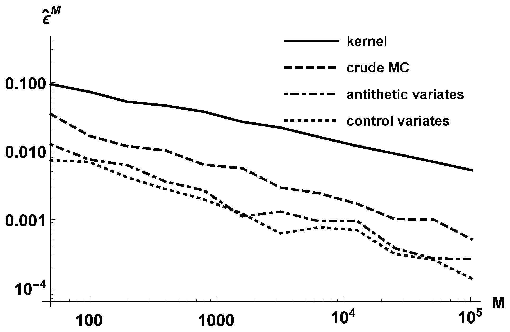Figure 1 reports the estimated error ${\widehat{ϵ}}^M$ in log-log scale, for different orders M growing geometrically. Observe that the parametric approach is more efficient than the kernel method. Variance reduction methods also allow for lowering the error. The lines corresponding to the three parametric methods have slope $-1/2$ approximately, due to the well-known decrease of the Monte Carlo error.

For example, to achieve an error ${ϵ}^M<0.01$, the kernel density estimation requires about $\mathrm{25,000}$ realizations, while the parametric crude Monte Carlo estimation needs 400 realizations. The antithetic method decreases the number of required realizations to 50–100, and the control variates approach does so even more, to less than 50.

In

Table 1. Time in seconds to achieve root mean square error less than 0.01 and 0.001. We employ a kernel method, parametric crude Monte Carlo (MC) simulation, antithetic variates and control variates methods. This table corresponds to Example 1.

Time	Kernel	Crude MC	Antithetic Variates	Control Variates
error 0.01	0.063	0.00089	0.00023	0.00015
error 0.001	4.2	0.13	0.012	$0.0057$

, we present the timings in seconds for achieving root mean square errors less than $0.01$ and $0.001$. We work at the density location $x=1$. Observe that the kernel density estimation is the least efficient method, especially as we require smaller errors.

Example 2.

Let $X=UV$, where $U\sim \mathrm{Normal}(0,1)$ and $V=P+{\sum }_{i=1}^{12}{Q}_i$, being $P\sim \mathrm{Poisson}\left(1\right)$ and $Q_i\sim \mathrm{Triangular}(0.1,0.105)$. All of the random variables are assumed to be independent. With $g(U,V)=UV$ and $h(U,V)=U/V$, expression (2) is $f_X\left(x\right)=\mathbb{E}\left[f_U\left(\frac{x}{V}\right)\frac{1}{V}\right]$. 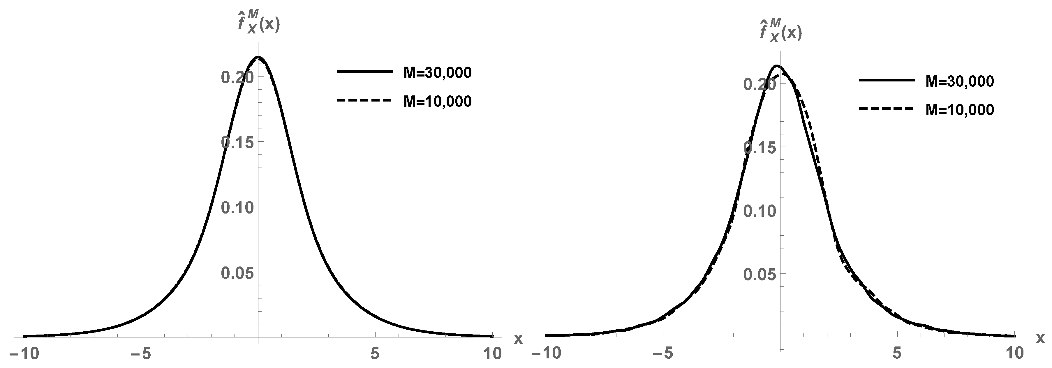Notice that, despite V being discrete, X has a density. This expectation cannot be computed via quadratures, due to the large dimension of the random space. We employ our parametric method using crude Monte Carlo simulation. In Figure 2, first panel, we depict the estimated density function ${\widehat{f}}_X^M\left(x\right)$ using M realizations. For $M=\mathrm{10,000}$ and $M=\mathrm{30,000}$, we perceive good agreement between the approximations. This is in contrast to the second panel of Figure 2, where the kernel density estimation does not show convergence yet.

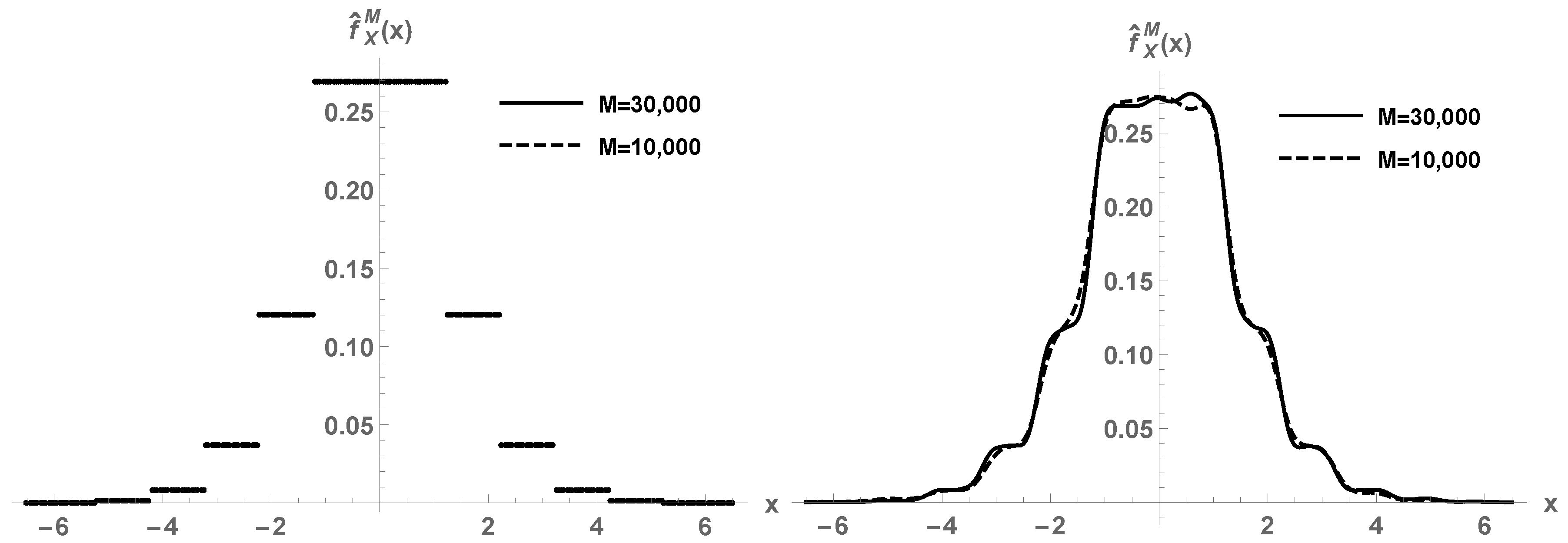
Example 3.

Consider the same setting of Example 2 but $U\sim \mathrm{Uniform}(-1,1)$ (now $f_U$ is not continuous on $\mathbb{R}$). In Figure 3, first plot, we show the estimated density function ${\widehat{f}}_X^M\left(x\right)$ by the parametric crude Monte Carlo method using M realizations. The discontinuity points of the target density $f_X$ are correctly captured. Indeed, the method acts pointwise in x, so any feature of $f_X$ will be correctly identified, no matter how rare it is. By contrast, the kernel density estimation smooths out the discontinuities, see the second panel of the figure.

4. Application to Random Differential Equations

A random differential equation problem considers some of the terms in the system (input coefficients, forcing term, initial conditions, etc.) as random variables or stochastic processes [1]. This is due to errors in measurements of data when trying to model a physical phenomenon, which introduces a variability in the parameters estimation. The solution to the system is then a stochastic process. Its deterministic trajectories are not the main concern. Instead, the study of the statistical content of the solution is the main goal. An important aim is to compute its probability density function. The key idea is that the solution is a transformation of the input random parameters; therefore, the probability density may be estimated as described in this paper whenever the solution is given in closed form. In the notation used in this paper, U and V would denote the input random parameters of the system, and g would be the transformation mapping that relates the output with the inputs. A specific input parameter is selected as U, with respect to which the mapping g is easily invertible to obtain h.

We consider the Ricatti random differential equation

$$\left\{\begin{array}{l}\dot{X}\left(t\right)=-AX{\left(t\right)}^2,t\in [0,\infty ),\\ X\left(0\right)=X_0,\end{array}\right.$$

(4)

where $A>0$ and $X_0$ are independent random variables. The solution to (4) is given by

$$X\left(t\right)=\frac{X_0}{1+A{X}_{0}t}.$$

By taking $U=X_0$, the density function of $X\left(t\right)$ is given by

$$f_{X\left(t\right)}\left(x\right)=\mathbb{E}\left[f_{X_0}\left(\frac{x}{1-Axt}\right)\frac{1}{{(1-Axt)}^2}\right].$$

From M realizations of A, say $A^{\left(1\right)},\dots ,A^{\left(M\right)}$, the expectation is estimated via crude Monte Carlo simulation:

$$f_{X\left(t\right)}\left(x\right)\approx \frac{1}{M}\sum _{i=1}^M{f}_{X_0}\left(\frac{x}{1-A^{\left(i\right)}xt}\right)\frac{1}{{(1-A^{\left(i\right)}xt)}^2}.$$

(5)

As seen in the previous sections, this procedure is more efficient and certain than kernel density estimation, expressed as

$$f_{X\left(t\right)}\left(x\right)\approx \frac{1}{Mb}\sum _{i=1}^{M}K\left(\frac{x-X_0^{\left(i\right)}/(1+A^{\left(i\right)}{X}_0^{\left(i\right)}t)}{b}\right),$$

where the superscript i denotes the i-th realization, $i=1,\dots ,M$.

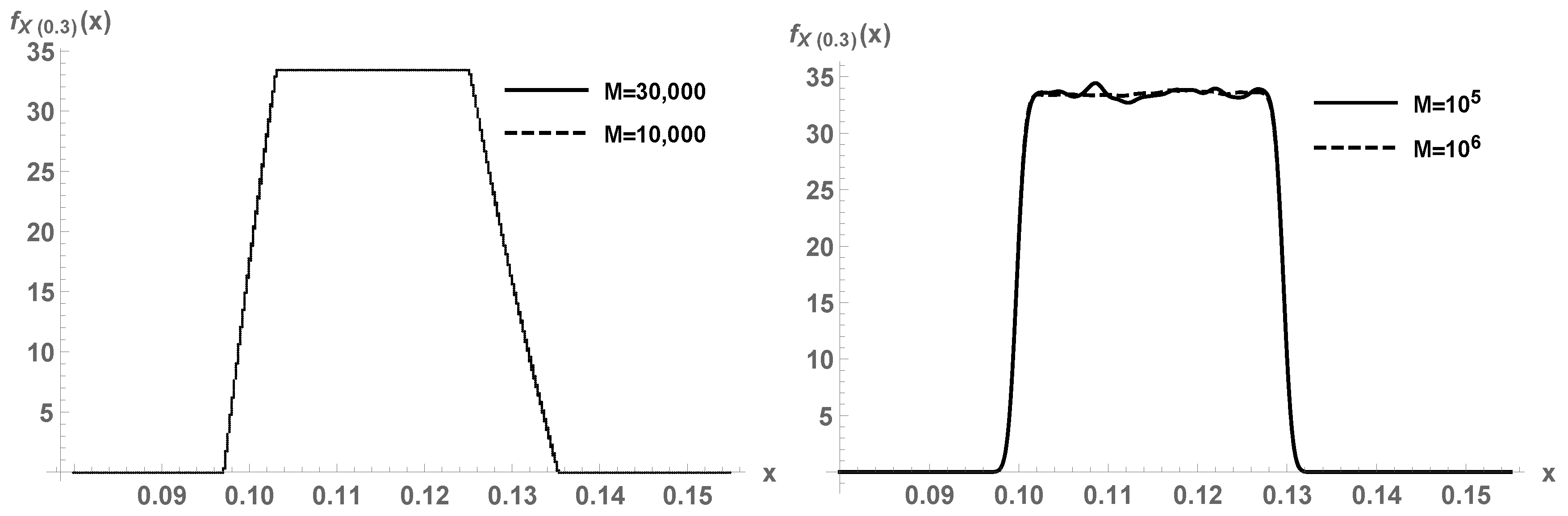
For a specific numerical example, let us fix $A\sim \mathrm{Uniform}(-1,1)$ and $X_0\sim \mathrm{Uniform}(0.1,0.13)$. Figure 4, first panel, plots (5) for a certain number of realizations M for A, for time $t=0.3$. A comparison is conducted with kernel density estimation with a Gaussian kernel (second panel). It must be appreciated that the parametric Monte Carlo method (5) correctly captures the non-differentiability points of the target density.

For another example, let us consider the damped pendulum differential equation with uncertainties:

$$\left\{\begin{array}{l}\ddot{X}\left(t\right)+2{\omega }_0\xi \dot{X}\left(t\right)+{\omega }_0^{2}X\left(t\right)=Y\left(t\right),t\in [0,T],\\ X\left(0\right)=X_0,\\ \dot{X}\left(0\right)=X_1,\end{array}\right.$$

(6)

where $T>0$, $w_0\ne 0$, $\xi \ne 0$ and ${\xi }^2<1$ (underdamped case) are constant, the initial position $X_0$ and the initial velocity $X_1$ are random variables, and the source/forcing term $Y\left(t\right)$ is a stochastic process ([1], Example 7.2). The solution is given by

$$X\left(t\right)=\left(\frac{\xi {\mathrm{e}}^{-{\omega }_0\xi t}sin\left({\omega }_{1}t\right)}{\sqrt{1-{\xi }^2}}+{\mathrm{e}}^{-{\omega }_0\xi t}cos\left({\omega }_{1}t\right)\right)X_0+\frac{{\mathrm{e}}^{-{\omega }_0\xi t}sin\left({\omega }_{1}t\right)}{{\omega }_1}{X}_1+{\int }_0^{t}p(t-s)Y\left(s\right)\mathrm{d}s,$$

(7)

where ${\omega }_1={\omega }_0\sqrt{1-{\xi }^2}\ne 0$ and $p\left(t\right)=\frac{1}{{\omega }_1}{\mathrm{e}}^{-\xi {\omega }_{0}t}sin\left({\omega }_{1}t\right)$. In [4], the density function of the response $X\left(t\right)$ is expressed in terms of an expectation (2), which is estimated by means of parametric crude Monte Carlo simulation due to the large dimension of the random space. By taking $U=X_0$, one of the formulas derived is

$$\begin{array}{ll}{f}_{X\left(t\right)}& \left(x\right)=\mathbb{E}\left[f_{X_0}\left(\frac{x-\frac{{\mathrm{e}}^{-{\omega }_0\xi t}sin\left({\omega }_{1}t\right)}{{\omega }_1}{X}_1-{\int }_0^{t}p(t-s)Y\left(s\right)\mathrm{d}s}{\frac{\xi {\mathrm{e}}^{-{\omega }_0\xi t}sin\left({\omega }_{1}t\right)}{\sqrt{1-{\xi }^2}}+{\mathrm{e}}^{-{\omega }_0\xi t}cos\left({\omega }_{1}t\right)}\right)\right]\frac{1}{\left|\frac{\xi {\mathrm{e}}^{-{\omega }_0\xi t}sin\left({\omega }_{1}t\right)}{\sqrt{1-{\xi }^2}}+{\mathrm{e}}^{-{\omega }_0\xi t}cos\left({\omega }_{1}t\right)\right|}\\ \approx & \frac{1}{M}\sum _{i=1}^M{f}_{X_0}\left(\frac{x-\frac{{\mathrm{e}}^{-{\omega }_0\xi t}sin\left({\omega }_{1}t\right)}{{\omega }_1}{X}_1^{\left(i\right)}-{\int }_0^{t}p(t-s)Y^{\left(i\right)}\left(s\right)\mathrm{d}s}{\frac{\xi {\mathrm{e}}^{-{\omega }_0\xi t}sin\left({\omega }_{1}t\right)}{\sqrt{1-{\xi }^2}}+{\mathrm{e}}^{-{\omega }_0\xi t}cos\left({\omega }_{1}t\right)}\right)\frac{1}{\left|\frac{\xi {\mathrm{e}}^{-{\omega }_0\xi t}sin\left({\omega }_{1}t\right)}{\sqrt{1-{\xi }^2}}+{\mathrm{e}}^{-{\omega }_0\xi t}cos\left({\omega }_{1}t\right)\right|},\hfill \end{array}$$

(8)

where the superscript i denotes the i-th realization, $i=1,\dots ,M$. Compare (8) with a kernel density estimation

$$f_{X\left(t\right)}\left(x\right)\approx \frac{1}{Mb}\sum _{i=1}^{M}K\left(\frac{x-\left(\frac{\xi {\mathrm{e}}^{-{\omega }_0\xi t}sin\left({\omega }_{1}t\right)}{\sqrt{1-{\xi }^2}}+{\mathrm{e}}^{-{\omega }_0\xi t}cos\left({\omega }_{1}t\right)\right)X_0^{\left(i\right)}-\frac{{\mathrm{e}}^{-{\omega }_0\xi t}sin\left({\omega }_{1}t\right)}{{\omega }_1}{X}_1^{\left(i\right)}-{\int }_0^{t}p(t-s)Y^{\left(i\right)}\left(s\right)\mathrm{d}s}{b}\right).$$

The expressions and their complexities are very similar, but the convergence of (8) is faster with M, as justified in the previous sections.

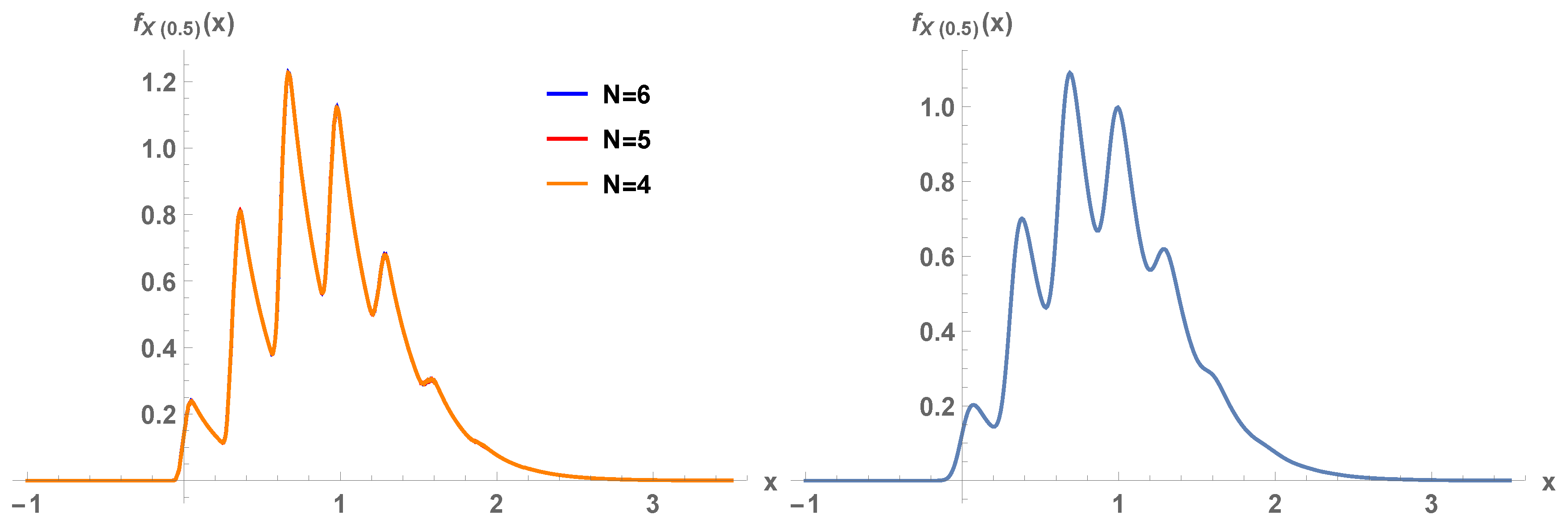
Let us see a numerical example. We take the upper time $T=1$, the damping ratio $\xi =1/2$ and the natural frequency ${\omega }_0=\pi /2$. Consider $X_0\sim \mathrm{Exponential}\left(3\right)$, $X_1\sim \mathrm{Binomial}(7,0.31)$ and $Y\left(t\right)={\sum }_{j=1}^{\infty }\frac{\sqrt{2}}{j\pi }sin\left(tj\pi \right){\xi }_j$. The series is understood in ${\mathrm{L}}^2([0,1]\times \Omega )$ and ${\left\{{\xi }_j\right\}}_{j=1}^{\infty }$ is a sequence of independent random variables with $\mathrm{Uniform}(-\sqrt{3},\sqrt{3})$ distribution. This is a Karhunen–Loève expansion ([10], p. 47). It is assumed that $X_0$, $X_1$, and Y are independent. By applying (8) with the sum of $Y\left(t\right)$ truncated to a finite-term series, we estimate the density function of $X\left(t\right)$. For example, in Figure 5, first panel, $f_{X\left(0.5\right)}\left(x\right)$ is plotted for orders of truncation $N=4$, 5, and 6. Overlapping of the graphs is clearly appreciated. The strong oscillations of the density are perfectly captured because the method acts pointwise. In the second panel of the figure, the kernel density estimate with Gaussian kernel is plotted, with ${10}^6$ realizations. Although there is apparent agreement between both panels, our parametric Monte Carlo method captures all the peaks while the kernel method smooths them out.

Further applications of the methodology for random differential equations may be consulted in [3,4,5,6,7]. The present paper forms the theoretical and computational foundations of the methodology used in those recent contributions.

5. Conclusions

In this paper, we have been concerned with the density estimation of random variables. We have proposed an alternative to kernel density estimation for certain random variable transformations. The alternative is based on the estimation of an expectation parameter via Monte Carlo methods; therefore, it is of parametric nature and improves kernel methods in terms of efficiency. Furthermore, the method captures density features and does not smooth out discontinuity and non-differentiability points of the target density.

As shown here, the solution to some random differential equation problems is an explicit transformation of the input random parameters. The methodology proposed in this paper may be employed to estimate the density function of the closed-form stochastic solution parametrically, instead of relying on kernel estimation.