Abstract
A model for tracking objects whose topological properties change over time is proposed. Such changes include the splitting of an object into multiple objects or the merging of multiple objects into a single object. The proposed model employs a novel formulation of the tracking problem in terms of homology theory whereby 0-dimensional homology classes, which correspond to connected components, are tracked. A generalisation of this model for tracking spatially close objects lying in an ambient metric space is also proposed. This generalisation is particularly suitable for tracking spatial-temporal phenomena such as rain clouds. The utility of the proposed model is demonstrated with respect to tracking communities in a social network and tracking rain clouds in radar imagery.
1. Introduction
The ability to accurately track objects is a fundamental requirement for many applications. For example, when attempting to make inferences with respect to future weather conditions, the ability to track weather phenomena, such as a snow storm, is necessary for predicting the future location of such phenomena [1]. When a robot is attempting to perform the task of object grasping and manipulation, the ability to accurately track the manipulator and target objects is necessary for generating and executing suitable motion plans [2]. Finally, when attempting to prevent the spread of an infectious disease, the ability to track social network communities is necessary to identify those most at risk and in turn take preventative measures.
In many instances of the object tracking problem, one cannot directly observe the objects in question. Instead, one typically indirectly observes the objects through sensor measurements at a sequence of discrete times (this is known as partial observability). In such cases, tracking requires that the set of objects plus their locations be inferred from these measurements at each time. It also requires that correspondences between the same object existing at different times be inferred. In many cases, object properties can change between consecutive times making it difficult to correctly infer these correspondences. For example, when tracking a person in a video sequence, both the appearance and shape of the person may change significantly over time. When tracking a weather phenomenon, both the shape and topology of the phenomenon may change significantly over time. In the context of this work, changes in the topology of an object include the formation of holes plus the splitting into and merging of multiple connected components. When attempting to track objects with changing properties, it is necessary to employ a method of tracking which is robust and can successfully track objects in the presence of such changes.
Many solutions to the problem of object tracking have been proposed which are robust with respect to changes in appearance and shape [3]. However, tracking objects robustly with respect to changes in topology represents an open research problem [4]. In this article, we propose a novel tracking model which is robust to such changes. The model assumes that the objects have been accurately modelled at a sequence of discrete times using a sequence of simplicial complexes. A simplicial complex is a general combinatorial representation capable of modelling a variety of types of objects and, as a consequence, the proposed model is a general model capable of tracking a variety of types of objects. We now illustrate the proposed model with respect to tracking objects in a graph.
Figure 1 illustrates the result of tracking objects in a graph at four consecutive discrete times using the proposed model where each vertex is labelled with a unique letter [5]. Note that the graph in question is not embedded in any space. In this case, individual objects correspond to connected components of the graph where the same object existing at multiple consecutive discrete times is represented using a single unique vertex colour. In the first discrete time, it is inferred that a single red object exists. In the second discrete time, it is inferred that the red object has split into red and blue objects. In the third discrete time, it is inferred that the blue object has grown in size. Finally, in the fourth discrete time, it is inferred that the blue and red objects have merged to form a single red object.
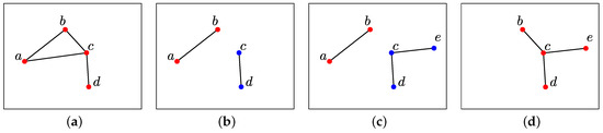
Figure 1.
The result of tracking objects in a graph at four consecutive discrete times using the proposed method is illustrated where each vertex is labelled with a unique letter. In this case, individual objects correspond to connected components of the graph where the same object existing at multiple consecutive discrete times is represented using a single unique vertex colour.
The proposed model formulates the problem of tracking in terms of homology theory, whereby it tracks 0-dimensional homology classes which correspond to connected components. Persistent homology is a commonly employed approach from homology theory to tracking homology classes of given dimension. However, in its native form, persistent homology is only capable of inferring the appearance and subsequent disappearance of such classes and cannot infer their locations [6]. Generalising persistent homology to overcome this limitation and perform object localisation represents the contribution of this article. For a given dimension, persistent homology returns a result that may be uniquely represented using a persistence diagram. A persistence diagram is a multiset of points where a point with coordinates indicates that a homology class of given dimension appeared at discrete time p and subsequently disappeared at discrete time q [7,8]. Similar to persistent homology, the proposed tracking method returns a result that may be uniquely represented using a persistence diagram. However, it also returns a map from points in the persistence diagram to corresponding homology classes. To illustrate this map, consider again the example of tracking objects in a graph described above. The corresponding persistence diagram is displayed in Figure 2. Each point in the persistence diagram has a colour equal to that of the object it maps to. For example, the blue point with coordinates (2, 4) in Figure 2 indicates that the blue object in Figure 1 appeared at discrete time 2 and disappeared at discrete time 4. Note that any object which exists at discrete time 4, which is the final discrete time, is determined to disappear at an unobserved discrete time 5. This is the case for the red object in Figure 1.
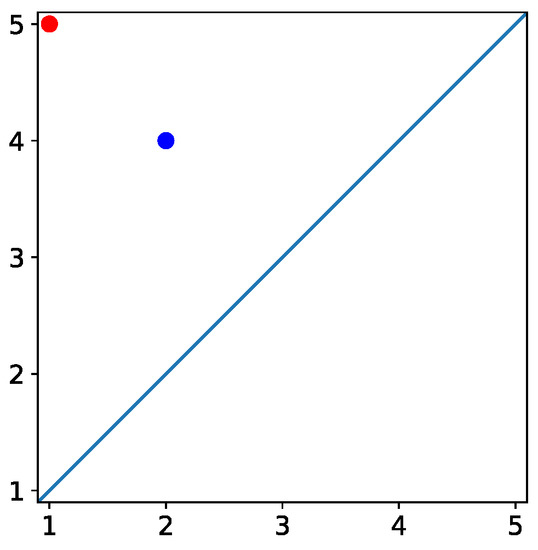
Figure 2.
The persistence diagram corresponding to the example of tracking objects in a graph of Figure 1 is displayed. Each point in the persistence diagrams has a colour equal to that of the object to which it maps.
The layout of this article is as follows. Section 2 reviews related works on homology theory and tracking objects robustly with respect to changes in topology. Section 3 describes the proposed tracking model. This section also describes a generalisation of this model for tracking objects in an ambient metric space where objects correspond to sets of spatially close homology classes. For many real world tracking problems, such as tracking weather phenomena, this is the more appropriate model. Section 4 presents an evaluation of the model and demonstrates application of the model to tracking communities in a social network and tracking rain clouds in radar imagery. Finally, Section 5 presents research conclusions and future research directions.
2. Related Works
This section presents a review of related approaches to modelling the topology of time series data and tracking objects with changing topological properties. Kramár et al. [9] employed persistent homology to study image time series data for different types of fluid dynamics. By measuring the Bottleneck distance between persistence diagrams corresponding to consecutive pairs of images, the authors were able to detect discontinuities in topological features. The authors also developed a tool called the TDA Persistence Explorer which allows one to identify with each point in the persistence diagram a pair of elements in the simplicial complex which caused the appearance and disappearance of the topological feature in question. Gonzalez-Diaz et al. [10] proposed a method for object tracking which is formulated in terms of persistent homology as opposed to zigzag persistent homology which is considered in this work. Their method is designed for tracking in image time series and is less general than that proposed in this work. Corcoran et al. [7] employed zigzag persistent homology to characterise the spatial-temporal behaviour of a swarm. However, the method proposed does not perform object localisation.
Several models for tracking objects with dynamic topology have been proposed by those working in the domain of Geographical Information Science (GIS). Liu et al. [11,12] proposed a tracking model which considers objects corresponding to multiple connected components. This model is conceptual in nature and no corresponding computational model is proposed. Worboys et al. [13] and Jiang et al. [14] proposed models for tracking topological changes in spatial phenomena using a geosensor network. These models are mostly conceptual in nature and cannot directly be applied to real data without further development. For example, the models proposed Worboys et al. [13] and Jiang et al. [14] assume a continuous representation of change in topology. This assumption is not exhibited by most real world data and consequently the authors limited their evaluation to simulated data. An important distinction between these and the proposed model is that these models are formulated in terms of logic while the proposed model is formulated in terms of homology theory.
There exist many techniques for performing clustering of spatial temporal data [15]. However, the problem of clustering assumes that object locations remain constant over time and is distinct from the problem of tracking.
3. Tracking Model
This section presents the proposed tracking model. The model assumes that the objects have been modelled at a sequence of discrete times using a sequence of simplicial complexes. In most real world scenarios, this sequence will be obtained by performing a triangulation of the objects in question where triangulation is the process of constructing a simplicial complex representation. As illustrated in Section 1, this is a very general representation which facilitates the tracking of a variety of types of objects.
This section is structured as follows. Section 3.1 presents background material on homology theory and formulates the problem of tracking in terms of computing maps between 0-dimensional homology classes which correspond to connected components. A fundamental component of computing these maps is the pullback of the zigzag diagram which is explained in Section 3.2. Subsequently, Section 3.3 describes how the pullback is employed to compute the maps in question. Section 3.4 describes how object tracking is inferred from these maps. Finally, Section 3.5 presents a generalisation of the proposed model for tracking objects in an ambient metric space where objects correspond to sets of spatially close homology classes.
3.1. Model Formulation
An (abstract) simplicial complex is a finite collection of sets such that for each all subsets of are also contained in . Each element is called a simplex or k-simplex where is the dimension of the simplex. The faces of a simplex correspond to all simplices where . The dimension of a simplicial complex is the largest dimension of any simplex .
A p-chain on a simplicial complex is defined in Equation (1) where each is a p-simplex and each is an element in a specified field. The set of p-chains forms a group called the chain group . The boundary map is a map from a p-simplex to the sum of its -simplex faces as defined in Equation (2). Here, is the -simplex obtained by deleting the 0-simplex from the p-simplex . This map is distributive and extends to the chain groups giving the sequence of chain groups in Equation (3).
A p-chain c is a p-cycle if and a p-boundary if there exists a -chain d where . The sets of all p-cycles and p-boundaries form groups which are denoted and , respectively. Each of these groups is a subgroup of . As a consequence of the fact , it can be proved that . The quotient group is a vector space and is called the p-dimensional homology group of . For those unfamiliar with homology theory, good introductions to the topic can be found in [16,17]. A useful introduction of the application of homology theory to graphs and networks can be found in [18]. The elements of are called p-dimensional homology classes. Each homology class is an equivalence class over cycles where two cycles in the same homology class are said to be homologous. This means they differ by a boundary [19]. A homology class of corresponds to a p-dimensional hole in the simplicial complex . Note that a homology class of corresponds to a connected component in the simplicial complex ; this is a consequence of the fact that all 0-simplices in a connected component differ by the boundary of a 1-chain equal to the sum of 1-simplices connecting the 0-simplices in question. The number of homology classes in is called the pth Betti-number. The focus of this article is tracking objects which we define as connected components; therefore, we consider the 0-dimensional homology classes and ignore higher order homology classes.
There exist a number of algorithms to compute the number and locations of the homology classes of for a given simplicial complex and dimension p [6]. In this work, we assume a sequence of n simplicial complexes obtained by triangulating the objects in question at a sequence of n discrete time steps. We wish to track 0-dimensional homology classes existing within this sequence. Toward this goal, for a given i in the range , we define an injective map which maps the homology classes of to the homology classes of . Given this, we formulate the problem of tracking as computing the sequence of maps defined in Equation (4) where . For , two connected components corresponding to a homology class in and a homology class in are determined to be the same object if and only if there exists a composition of maps between the homology classes in question.
3.2. Pullback of the Zigzag Diagram
Before defining computation of the maps , we first define the pullback which is a subspace of the direct sum of 0-dimensional homology groups in question. Toward this goal we first construct the zigzag diagram of simplicial complexes with inclusion maps defined in Equation (5) [20]. Note that and are subcomplexes of . The term zigzag refers to the fact that the sequence of maps do not have a uniform direction and instead point in both forward and backward directions. As is illustrated in the next section, the mapping of consecutive simplicial complexes to their union in the zigzag diagram facilitates the definition of the required map between homology classes. By applying the 0-dimensional homology functor to the zigzag diagram of Equation (5), this gives the zigzag diagram of homology groups with induced linear maps defined in Equation (6) [20].
Let and be a pair of consecutive simplicial complexes in the sequence of simplicial complexes; that is, . Furthermore, let f and g be the inclusion maps defined in Equation (7), and let and be the induced maps defined in Equation (8). Recall that 0-dimensional homology classes correspond to connected components. Both and are surjective maps which map a 0-dimensional homology class in the domain to a 0-dimensional homology class in the codomain if and only if the connected component corresponding to the former is a subset of the connected component corresponding to the latter. This property is a consequence of the fact that individual 0-dimensional homology classes correspond to connected components. That is, the images of the inclusion maps f and g applied to two connected components differ by a 1-chain if they map to the same path connected component ([21], page 64).
To illustrate the maps and , consider the example in Figure 3. Here, simplicial complexes corresponding to and are represented in Figure 3a,b, respectively, and their union is represented in Figure 3c. In the figure, individual path-connected components are labelled with a unique letter in the range a–g. In this example, f maps the 0-dimensional homology classes corresponding to the connected components a and b in to the 0-dimensional homology classes corresponding to the connected components f and g in , respectively. Similarly, g maps the 0-dimensional homology classes corresponding to the connected components c and d in to the 0-dimensional homology class corresponding to the connected component f in . It also maps the 0-dimensional homology class corresponding to the connected component e in to the 0-dimensional homology class corresponding to the connected component g in .
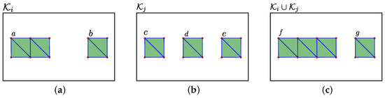
Figure 3.
Two simplicial complexes and and their union are displayed in (a–c), respectively. Red dots represent 0-simplices, blue lines represent 1-simplices and green triangles represent 2-simplices.
The pullback P of the maps f and g is defined in Equation (9) and is a subspace of the direct sum [22]. Specifically, the pullback is the set of all pairs of 0-dimensional homology classes of and which map to the same 0-dimensional homology class of . To illustrate the pullback consider again the example provided in Figure 3. Here, the pullback is where 0-dimensional homology classes are stated in terms of the labels of the connected components they correspond to.
3.3. Map of Homology Groups
Each element in the pullback P defines a map from an element of to an element of . That is, if , this defines a map from to . Recalling that , if we were to construct the required map to be union of all elements in the pullback, this might not be an injective map (A map is injective if and only if every element of the map’s codomain is the image of at most one element of its domain and furthermore the image of every element of the map’s domain is at most one element of its codomain). For example, if a connected component splits into two connected components, the pullback will contain two elements and the resulting map will not satisfy the property that the image of every element of the map’s domain is at most one element of its codomain. Persistent homology computes an injective map between homology classes [8]. To maintain consistency with persistent homology, we construct the required map to be injective by assigning it to be the union of a subset of the maps defined by the elements in the pullback. This subset is constructed using that outlined in Algorithm 1, which employs a heuristic giving preference with respect to persistence homology classes which firstly have persisted for longer and secondly correspond to larger connected components.
Algorithm 1 first defines independent total orders on the elements of and (Lines 3 and 4). A total order on the elements of is defined using the lexicographical order over the time since appearing followed by the size of the corresponding connected component. A homology class appears at if its preimage under the map is the empty set. A total order on the elements of is defined using the order over size of the corresponding connected components. To illustrate these independent orderings, consider again the example of Figure 3. Assume the homology class corresponding to the connected component a was born before that corresponding to the connected component b. In this case, the total order on the homology classes of will be that corresponding to a followed by that corresponding to b. As a consequence of the fact that all the connected components in are of equal size, any ordering of the homology classes in question is valid.
Given the total orders defined above, a total order on the elements of the pullback P is defined using the lexicographical order (Line 5). These elements are then iterated through in decreasing order (Line 6) and each element is added to the map if its addition does not invalidate the injective property (Lines 7 and 8).
| Algorithm 1: Compute Map . |
 |
To illustrate the construction of , consider again the example provided in Figure 3 where the pullback is . Here, the lexicographical order is and as a consequence the subset used to construct is .
3.4. Tracking
As stated in the model formulation of Section 3.1, for , homology classes in and are determined to be the same object if and only if there exists a compositions of maps between the homology classes in question. Given this, we compute the set of homology classes corresponding to each object in the sequence using the approach outlined in Algorithm 2.
Algorithm 2 first constructs a graph where the set of vertices V correspond to homology classes and the set of edges E correspond to the existence of a map between the homology classes in question (Lines 2–12). Each connected component in this graph corresponds to an individual object and the set of homology classes contained in a given connected component equals those corresponding to the object in question. The connected components in G are computed using a breadth first search and the set of homology classes in each of these components is constructed (Lines 13–16). Finally, Algorithm 2 returns R, which equals a set of sets (Line 17).
Given the result of Algorithm 2, it is straight forward to compute the persistence diagram for the 0-dimensional homology group. There exists a bijective map between points in the persistence diagram and 0-dimensional homology classes. A point with coordinates in the persistence diagram indicates that the corresponding homology class appeared and disappeared, respectively, at simplicial complexes with indices p and q, respectively. If a 0-dimensional homology class appears in but never disappears, it is represented as a point in the persistence diagram with coordinates . That is, we assume it disappears in a subsequent simplicial complex , which is not observed. For a given point in a persistence diagram, the value is referred to as the persistence of the homology class in question.
| Algorithm 2: Tracking in sequence . |
 |
Consider again the example in Figure 3 where individual connected components are labelled with a unique letter in the range a–g and let the indices i and j of the simplicial complexes in question be 1 and 2, respectively. The persistence diagram corresponding to this sequence of simplicial complexes will contain three points with coordinates (1, 3), (1, 3) and (2, 3). Here, we are assuming that all 0-dimensional homology classes which exist in disappear in which is not observed. One of the two points with coordinates (1, 3) corresponds to the object with connected components a and c. The other point with coordinates (1, 3) corresponds to the object with connected components b and e. Finally, the point with coordinates (2, 3) corresponds to the object with the connected component d.
There is a map from points in a persistence diagram to 0-dimensional homology classes. As illustrated in the example of tracking objects in a graph presented in Section 1, it is possible to make this map explicit when visualising the data in question. This is achieved by colouring each point in the persistence diagram with a unique colour and subsequently colouring all 0-dimensional homology classes correspond to that point with the same colour.
3.5. Tracking in a Metric Space
In many instances of the tracking problem, the objects in question lie in an ambient metric space where an individual object might not correspond to a single 0-dimensional homology class but instead a set of such classes which are spatially close. For example, the problem of tracking a rainstorm may be formulated in terms of tracking a set of homology classes or connected components in which are spatially close and where each corresponds to an individual rain cloud. In this section, we propose a generalisation of the proposed tracking method capable of tracking such objects corresponding to spatially close homology classes.
In the original model, we assume a sequence of n simplicial complexes obtained by triangulating connected components at a sequence of n discrete time steps. In the generalised model, we assume an additional sequence of n simplicial complexes obtained by triangulating an enlargement of the original connected components at the same sequence of discrete times. The consequence of this enlargement is that very close objects will merge to form a single homology class. The enlargement may be defined as the subset of the ambient space that is within a specified distance of the connected components. Alternatively, if the connected components are defined on a regular grid or image/array the enlargement may be defined as the morphology dilation. The relationship between these two sequences of simplicial complexes is that spatially close connected components in a given will form a single larger connected component in . To illustrate consider the sequence of simplicial complexes and represented in Figure 4a,b, respectively, plus the corresponding sequence of simplicial complexes and represented in Figure 4c,d, respectively. The connected components labelled a and b in are spatially close and consequently form a single larger connected component labelled g in . Similarly, the connected components labelled d and e in are spatially close and consequently form a single larger connected component labelled r in .
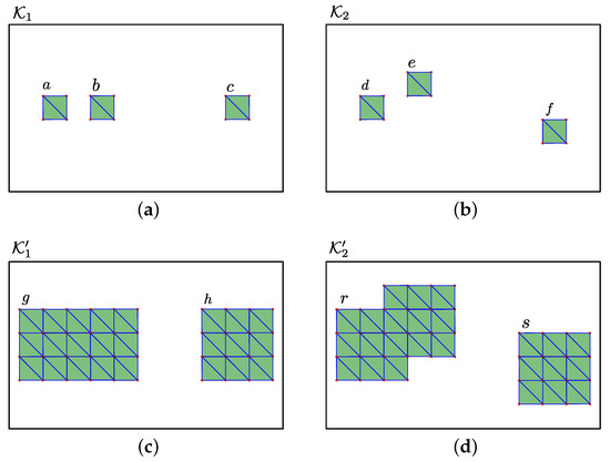
Figure 4.
The simplicial complexes and in (a), (b), respectively, correspond to the triangulation of objects at two discrete time steps. The simplicial complexes and in (c), (d), respectively, correspond to the triangulation of an enlargement of objects at the same two discrete time steps. Each connected component is labelled with a unique letter.
In the generalised tracking model, we apply the original tracking model to the sequence of simplicial complexes . Recall that this model will compute the set of homology classes corresponding to each object in the sequence . For example, applying the original tracking model to the sequence in Figure 4 computes that two objects exists in the sequence where one object corresponds to the homology classes with labels g and r while the other corresponds to the homology classes with labels h and s.
We next propagate the result of this tracking to the sequence using that outlined in Algorithm 3. For each subset of homology classes r in the sequence corresponding to an individual object in that sequence, a corresponding subset of homology classes in the sequence is constructed (Lines 3–5). Specifically, a homology class in the sequence is included in this set if it is a subset of a homology class in the set r. This subset evaluation assumes an inclusion map of into . This map will be surjective because the homology classes in are enlarged in . Applying this propagation to the example in Figure 4 computes that two objects exists in the sequence where one object corresponds to the connected components with labels a, b, d and e while the other corresponds to the connected components with labels c and f.
| Algorithm 3: Propagate tracking in sequence to sequence . |
 |
4. Results
This section presents an evaluation of the proposed tracking model implementation and demonstrates the applicability of this model to real world tracking problems. Section 4.1 evaluates the accuracy of the model implementation using random small scale instances for which results may be compared to manually generated ground truth. Section 4.2 describes the application of the tracking model to a temporal network corresponding to a real online social network. Finally, Section 4.3 describes the application of the generalised model described in Section 3.5 to rainfall radar data obtained from the UK Meteorological (Met) Office.
4.1. Model Accuracy
This section describes a set of experiments performed to evaluate the accuracy of the tracking model implementation. In each experiment, a sequence of random simplicial complexes of dimension 1 was generated. The model was applied to each sequence and the resulting persistence diagrams were manually compared to corresponding ground truth persistence diagrams. The ground truth persistence diagrams in question were manually generated. Note that, since tracking is modelled in terms of elements of the 0-dimensional homology classes, it is not necessary to consider simplicial complexes of dimension greater than 1.
The following procedure was employed to generate each sequence of n random simplicial complexes. First, a set of m 0-simplices was generated and in turn used to generate a set of 1-simplices . Finally, each simplicial complex was generated by initialising it to be empty and adding the closure of each 1-simplex in the above set randomly with probability p. In all experiments, values of 5, 10 and 0.05 were assigned to the variables n, m and p, respectively. Figure 5 displays a sequence of four random simplicial complexes generated using this procedure.
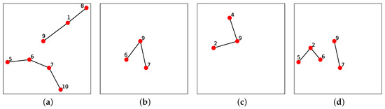
Figure 5.
A sequence of four random simplicial complexes , , and is displayed in (a–d), respectively. Each 0-simplex is represented by a red dot and labelled with its corresponding index i. Each 1-simplex is represented by a black line segment joining the corresponding two 0-simplex faces. The positioning of each simplicial complex was determined using the force-directed graph drawing algorithm [23].
For a given sequence of random simplicial complexes, in order to facilitate a comparison to ground truth, the proposed tracking model plus corresponding persistence diagram were visualised using the following procedure. The set of objects were sorted in ascending order based on the index i of the simplicial complex in which they appeared. If more than one object appeared in a single simplicial complex, the objects in question were randomly ordered. The objects were then mapped to integer values equalling their position in this ordering. That is, the first object that appeared was mapped to the value 1, the second object that appeared was mapped to the value 2, etc. Through a composition of maps, these integer values were in turn mapped to RGB colour values in a colour map that exhibits the property that similar values are mapped to similar colours. This has the effect of mapping objects that appeared at similar indexes to similar colours. Using this mapping from objects to colours, each 0-simplex and point in the persistence diagram was coloured according to the object it was determined to correspond to. This allows the visual mapping between objects in the sequence of simplicial complexes and corresponding points in the persistence diagram. In this work, we used a jet colour map. The positioning of each simplicial complex was determined using the force-directed graph drawing algorithm [23].
To illustrate this visualisation procedure, consider Figure 6, which visualises the proposed tracking model applied to the sequence of four simplicial complexes in Figure 5. The persistence diagram corresponding to this tracking is displayed in Figure 7. In , two objects appear and these are coloured blue and green. In , these objects merge to form a single object coloured blue. In , a single blue coloured object exists. Finally, in , this object splits to form two objects coloured blue and red. For this sequence of random simplicial complexes, the proposed tracking model equals the expected tracking.
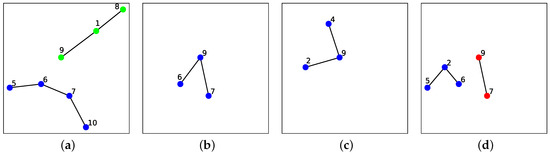
Figure 6.
The proposed tracking model applied to the sequence of four simplicial complexes in Figure 5 is displayed. Each 0-simplex is uniquely coloured according to the object to which it corresponds.
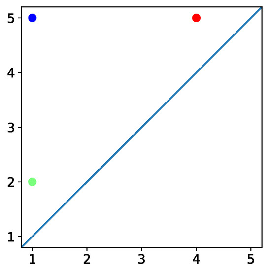
Figure 7.
The persistence diagram corresponding to the tracking of Figure 6 is displayed and contains three points.
The above experiment was repeated 25 times and in all cases the proposed tracking model equalled the expected tracking. This demonstrates the implementation accuracy of the proposed tracking model.
4.2. Tracking Temporal Network
This section describes the application of the proposed tracking model to the temporal network described in [24] and hosted by the Stanford Network Analysis Project (https://snap.stanford.edu/data/CollegeMsg.html). The network in question is a multigraph where vertices correspond to users of an online social network and edges correspond to messages sent between users. Each edge is labelled with the time, represented as a Unix timestamp, at which the message in question was sent. Given this network, we constructed a sequence of n simplicial complexes of dimension 1 using the following procedure.
Let and equal the minimum and maximum times, respectively, at which a message was sent and let equal . We subdivided the interval into n subintervals where . For each subinterval , we triangulated the subset of the network active during this subinterval as follows. We constructed a simplicial complex containing a 0-simplex corresponding to each user who exchanged a message during the interval plus a 1-simplex corresponding to each pair of users who exchanged a message during the interval where the two 0-simplex faces correspond to the users in question.
For the sequence of simplicial complexes , application of the proposed tracking model was visualised using the procedure described in Section 4.1. That is, each 0-simplex and point in the persistence diagram was coloured according to the object to which it was determined to correspond where objects that appear at similar times are mapped to similar colours.
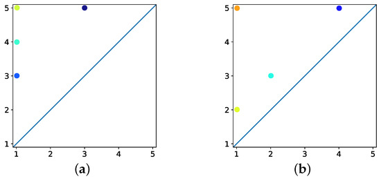
For a value of n equal to 20, visualisations of simplicial complexes , , and are displayed in Figure 8. The corresponding persistence diagram is displayed in Figure 9a. Recall that, if an object appears in but never disappears, it is represented as a point in the persistence diagram with coordinates . That is, it is assumed to disappear in a subsequent simplicial complex , which is not observed. Through inspection of the persistence diagram, we observe that a small subset of objects persist for significantly longer than other objects. One of these objects persists over the entire sequence and is coloured dark blue. This object is evident in the set of simplicial complexes of Figure 8.
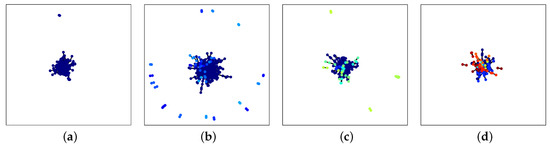
Figure 8.
The simplicial complexes , , and corresponding to the temporal network described in Section 4.2 are visualised in (a)–(d), respectively. The number of 0-simplexes in each of these simplicial complexes is 235, 402, 241 and 159, respectively. The number of connected components in each of these simplicial complexes is 4, 28, 17 and 21, respectively.
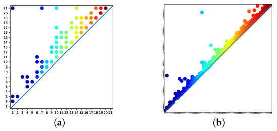
For a value of n equal to 100, visualisations of simplicial complexes , , and are displayed in Figure 10. The corresponding persistence diagram is displayed in Figure 9b. Again, through inspection of the persistence diagram, we observe that a small subset of objects persist for significantly longer than other objects. Two of these objects are coloured dark and light blue, respectively, and are evident in the set of simplicial complexes of Figure 10.
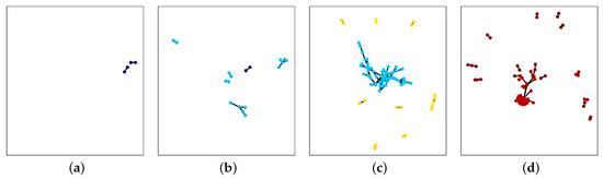
Figure 10.
The simplicial complexes , , and corresponding to the temporal network described in Section 4.2 are visualised in (a)–(d), respectively. The number of 0-simplexes in each of these simplicial complexes is 4, 18, 75 and 66, respectively. The number of connected components in each of these simplicial complexes is 2, 6, 10 and 15, respectively.
4.3. Tracking Rain Clouds
This section describes the application of the generalised model, described in Section 3.5, to rainfall radar images obtained from the UK Meteorological (Met) Office [25]. The Met office updates the data every 15 min with a 15-min delay due to processing time. For a given time, the image data in question categorise the rainfall at each location in a 500 × 500 regular grid over Ireland and the UK. Specifically, the level of rainfall is one of eight categories based on the number millimetres per hour (mm/h) of rainfall at that location. For the purposes of applying the proposed tracking model, we converted the original categorisation of rainfall level to a binary categorisation corresponding to the categorises of less than 0.01 mm/h of rainfall and greater than or equal to 0.01 mm/h of rainfall. The threshold value of 0.01 mm/h was chosen because the Met office categorises levels of rainfall less than this value as no rainfall.
Given these data, we considered the problem of tracking objects corresponding to spatially close connected components of with a rainfall level greater than this threshold. Recall that the generalised tracking model requires that at each time we triangulate both the original and enlarged connected components. We triangulated the original connected components using the following procedure. If a location in the regular grid was greater than or equal to the threshold, a corresponding 0-simplex was added. If the rainfall at two horizontally or vertically adjacent locations was greater than or equal to the threshold, a 1-simplex was added where the two 0-simplex faces correspond to the locations in question. The enlarged connected components were constructed by performing a binary morphology dilation of the gird of points with a rainfall level greater than the threshold [26]. Specifically, six iterations of binary dilation using a 3 × 3 structuring element with connectivity 1 were applied. The enlarged connected components were triangulated using the same procedure described above for triangulating the original connected components.
Figure 11 and Figure 12 illustrate the application of the model to two short sequences of rainfall radar images. The persistence diagrams corresponding to these figures are displayed in Figure 13a,b, respectively. In these figures, all connected components corresponding to the same object are uniquely coloured. It is evident from these figures that the model accurately tracks objects corresponding to spatially close connected components. For example, the connected components in the centre of the radar images of Figure 11 are spatially close and are correctly determined to correspond to a single object, which is coloured orange. A video clip displaying a longer tracking sequence can be viewed online at the following URL: https://youtu.be/w_IZSZEzAsg.
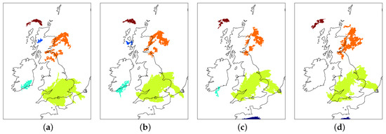
Figure 11.
The robust tracking of objects in a sequence of four rain radar images is illustrated. The objects in question correspond to spatially close connected components and are uniquely coloured.
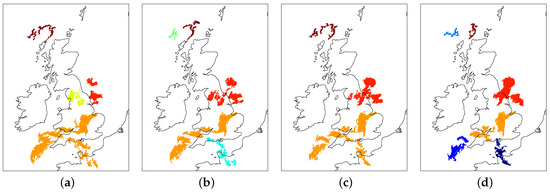
Figure 12.
The robust tracking of objects in a sequence of four rain radar images is illustrated. The objects in question correspond to spatially close connected components and are uniquely coloured.
5. Conclusions
As stated in Section 1, the ability to accurately track objects is a fundamental requirement for many applications. The tracking model proposed in this article offers a solution to the problem of tracking objects whose topological properties change over time. Many real world phenomena exhibit this property and therefore the proposed model has many potential applications. This includes tracking social networks and weather phenomena, which are briefly examined in Section 4. In future work, we plan to examine these and other applications in greater detail. To support application of the proposed tracking model to other problems, a pure Python implementation plus sample data will be made freely available on GitHub.
Conflicts of Interest
The authors declare no conflict of interest.
References
- Faghmous, J.H.; Kumar, V. Spatio-temporal data mining for climate data: Advances, challenges, and opportunities. In Data Mining and Knowledge Discovery for Big Data; Springer: Berlin, Germany, 2014; pp. 83–116. [Google Scholar]
- Cifuentes, C.G.; Issac, J.; Wüthrich, M.; Schaal, S.; Bohg, J. Probabilistic articulated real-time tracking for robot manipulation. IEEE Robot. Autom. Lett. 2017, 2, 577–584. [Google Scholar] [CrossRef]
- Yilmaz, A.; Javed, O.; Shah, M. Object tracking: A survey. ACM Comput. Surv. 2006, 38, 13. [Google Scholar] [CrossRef]
- Corcoran, P.; Jones, C.B. Robust Tracking of Objects with Dynamic Topology. In Proceedings of the 26th ACM SIGSPATIAL International Conference on Advances in Geographic Information Systems, Seattle, WA, USA, 6–9 November 2018; pp. 428–431. [Google Scholar] [CrossRef]
- Giblin, P. Graphs, Surfaces and Homology: An Introduction to Algebraic Topology; Springer Science & Business Media: Amsterdam, The Netherlands, 2013. [Google Scholar]
- Zomorodian, A.; Carlsson, G. Localized homology. Comput. Geom. 2008, 41, 126–148. [Google Scholar] [CrossRef]
- Corcoran, P.; Jones, C.B. Spatio-temporal modeling of the topology of swarm behavior with persistence landscapes. In Proceedings of the ACM SIGSPATIAL International Conference on Advances in Geographic Information Systems, Burlingame, CA, USA, 31 October–3 November 2016; p. 65. [Google Scholar]
- Corcoran, P.; Jones, C.B. Modelling topological features of swarm behaviour in space and time with persistence landscapes. IEEE Access 2017, 5, 18534–18544. [Google Scholar] [CrossRef]
- Kramár, M.; Levanger, R.; Tithof, J.; Suri, B.; Xu, M.; Paul, M.; Schatz, M.F.; Mischaikow, K. Analysis of Kolmogorov flow and Rayleigh–Bénard convection using persistent homology. Phys. D Nonlinear Phenom. 2016, 334, 82–98. [Google Scholar] [CrossRef]
- Gonzalez-Diaz, R.; Jimenez, M.J.; Medrano, B. Topological tracking of connected components in image sequences. J. Comput. Syst. Sci. 2018. [Google Scholar] [CrossRef]
- Liu, H.; Schneider, M. Detecting the Topological Development in a Complex Moving Region. J. Multimed. Process. Technol. 2010, 1, 160–180. [Google Scholar]
- Liu, H.; Schneider, M. Tracking continuous topological changes of complex moving regions. In Proceedings of the 2011 ACM Symposium on Applied Computing, Taichung, Taiwan, 21–25 March 2011; pp. 833–838. [Google Scholar]
- Worboys, M.; Duckham, M. Monitoring qualitative spatiotemporal change for geosensor networks. Int. J. Geogr. Inf. Sci. 2006, 20, 1087–1108. [Google Scholar] [CrossRef]
- Jiang, J.; Worboys, M. Event-based topology for dynamic planar areal objects. Int. J. Geogr. Inf. Sci. 2009, 23, 33–60. [Google Scholar] [CrossRef]
- Birant, D.; Kut, A. ST-DBSCAN: An algorithm for clustering spatial–temporal data. Data Knowl. Eng. 2007, 60, 208–221. [Google Scholar] [CrossRef]
- Patania, A.; Vaccarino, F.; Petri, G. Topological analysis of data. EPJ Data Sci. 2017, 6, 7. [Google Scholar] [CrossRef]
- Otter, N.; Porter, M.A.; Tillmann, U.; Grindrod, P.; Harrington, H.A. A roadmap for the computation of persistent homology. EPJ Data Sci. 2017, 6, 17. [Google Scholar] [CrossRef]
- Aktas, M.E.; Akbas, E.; El Fatmaoui, A. Persistence homology of networks: Methods and applications. Appl. Netw. Sci. 2019, 4, 61. [Google Scholar] [CrossRef]
- Hatcher, A. Algebraic Topology; Cambridge University Press: Cambridge, UK, 2002. [Google Scholar]
- Carlsson, G.; De Silva, V. Zigzag persistence. Found. Comput. Math. 2010, 10, 367–405. [Google Scholar] [CrossRef]
- Munkres, J. Elements of Algebraic Topology; Westview Press: Boulder, CO, USA, 1996. [Google Scholar]
- Vejdemo-Johansson, M.; Skraba, P. Parallel & scalable zig-zag persistent homology. In Proceedings of the NIPS Workshop on Algebraic Topology and Machine Learning, Lake Tahoe, NV, USA, 7–8 December 2012. [Google Scholar]
- Fruchterman, T.M.; Reingold, E.M. Graph drawing by force-directed placement. Softw. Pract. Exp. 1991, 21, 1129–1164. [Google Scholar] [CrossRef]
- Panzarasa, P.; Opsahl, T.; Carley, K.M. Patterns and dynamics of users’ behavior and interaction: Network analysis of an online community. J. Assoc. Inf. Sci. Technol. 2009, 60, 911–932. [Google Scholar] [CrossRef]
- Weather and Climate Data. Available online: https://www.metoffice.gov.uk/datapoint (accessed on 17 September 2019).
- Haralick, R.M.; Sternberg, S.R.; Zhuang, X. Image analysis using mathematical morphology. IEEE Trans. Pattern Anal. Mach. Intell. 1987, PAMI-9, 532–550. [Google Scholar] [CrossRef]


© 2019 by the author. Licensee MDPI, Basel, Switzerland. This article is an open access article distributed under the terms and conditions of the Creative Commons Attribution (CC BY) license (http://creativecommons.org/licenses/by/4.0/).