1. Introduction
Recent decades have seen the frontiers of scientific computing increasingly push towards the use of larger and larger datasets. In fact, frequently, the data to be represented are so large that they cannot fully fit into working memory. Fortunately, in many cases, the data have many zeros and can be represented in a compact manner, allowing users to work with sparse matrices of an extreme size with few non-zero elements. However, converting code from using dense matrices to using sparse matrices, a common task when scaling code to larger data, is not always straightforward.
Current open-source frameworks may provide several separate sparse matrix classes, each with its own data storage format. For example, SciPy [
1] has seven sparse matrix classes, where each storage format is best suited for efficient execution of a specific set of operations (e.g., incremental matrix construction vs. matrix multiplication). Other frameworks may provide only one sparse matrix class, with considerable runtime penalties if it is not used in the right way. This can be challenging and bewildering for users who simply want to create and use sparse matrices and do not have the time, expertise, nor desire to understand the advantages and disadvantages of each format. To achieve good performance, several formats may need to be used in one program, requiring explicit selection and conversion between the formats. This multitude of sparse matrix classes complicates the programming task, adds to the maintenance burden, and increases the likelihood of bugs.
Driven by the above concerns, we devised a practical and user-friendly sparse matrix class for the C++ language [
2]. The sparse matrix class uses a hybrid storage framework, which automatically and seamlessly switches between three data storage formats, depending on which format is best suited and/or available for specific operations:
Compressed Sparse Column (CSC), used for efficient and nuanced implementation of core arithmetic operations such as matrix multiplication and addition, as well as efficient reading of individual elements;
Red-Black Tree (RBT), used for both robust and efficient incremental construction of sparse matrices (i.e., construction via setting individual elements one-by-one, not necessarily in order);
Coordinate list (COO), used for low-maintenance and straightforward implementation of relatively complex and/or lesser-used sparse matrix functionality.
The COO format is important to point out, as the source code for the sparse matrix class is distributed and maintained as part of the open-source Armadillo library (
arma.sourceforge.net) [
3]. Due to its simpler nature, the COO format facilitates functionality contributions from time-constrained and/or non-expert users, as well as reducing maintenance and debugging overhead for the library maintainers.
To further promote efficient execution, the sparse matrix class internally implements a delayed evaluation framework [
4] based on template meta-programming [
5,
6] combined with operator overloading [
2]. In delayed evaluation, the evaluation of a given compound mathematical expression is delayed until its value is required (i.e., assigned to a variable). This is in contrast to eager evaluation (also known as strict evaluation), where each component of a compound expression is evaluated immediately. As such, the delayed evaluation framework allows automatic compile-time analysis of compound expressions, which in turn allows for automatic detection and optimisation of common expression patterns. For example, several operations can be combined to reduce the required computational effort.
Overall, the sparse matrix class and its associated functions provide a high-level application programming interface (function syntax) that is intuitive, close to a typical dense matrix interface, and deliberately similar to MATLAB. This can help with rapid transition of dense-specific code to sparse-specific code, facilitates prototyping directly in C++, and aids the conversion of research code into production environments.
While there are many other sparse matrix implementations in existence, to our knowledge, the presented approach is the first to offer a unified interface with automatic format switching under the hood. Most toolkits are limited to either a single format or multiple formats between which the user must manually convert. The comprehensive SPARSKIT package [
7] contains 16, and SciPy contains seven formats [
1]. In these toolkits, the user must manually convert between formats. On the other hand, both MATLAB and GNU Octave [
8] contain sparse matrix implementations, but they supply only the CSC format [
9], meaning that users must write their code in special ways to ensure its efficiency [
10]. This is a similar situation to the Blaze library (
bitbucket.org/blaze-lib/blaze) [
11], which uses a compressed format with either column- or row-major orientation. Users are explicitly discouraged from individual element insertions and, for efficiency, must construct their sparse matrices in a restricted and cumbersome environment of batch insertion. Furthermore, simply reading elements from the matrix via standard row and column indexing can result in temporary insertion of elements into the matrix. The Eigen C++ matrix library (
eigen.tuxfamily.org) uses a specialised sparse matrix format that has deliberate redundancy and overprovisioned storage. While this can help with reducing the computational effort of element insertion in some situations, it requires manual care to maintain storage efficiency. Furthermore, as the cost of random insertion of elements is still high, the associated documentation recommends manually constructing a COO-like representation of all the elements, from which the actual sparse matrix is then constructed. The IT++ library (
itpp.sourceforge.net) has a cumbersome sparse matrix class with a custom compressed column format that also employs overprovisioned storage. The format is less efficient storage wise than CSC unless explicit manual care is taken. Data are stored in an unordered fashion, which allows for faster element insertion than CSC, but at the cost of reduced performance for linear algebra operations. Overall, the landscape of sparse matrix implementations is composed of libraries where the user must be aware of some of the internal storage details and the associated maintenance in order to produce efficient code; this is not ideal.
To make the situation even more complex, there are also numerous other sparse matrix formats [
7,
12,
13]. Examples include the modified compressed row/column format (intended for sparse matrices where the main diagonal has all non-zero elements), block compressed storage format (intended for sparse matrices with dense submatrices), diagonal format (intended for straightforward storage of banded sparse matrices under the assumption of constant bandwidth), and the various skyline formats (intended for more efficient storage of banded sparse matrices with irregular bandwidth). As these formats are focused on specialised use cases, their utility is typically not very general. Thus, we have currently opted against including these formats in our hybrid framework, though it would be relatively easy to accommodate more formats in the future.
The paper is continued as follows. In
Section 2, we overview the functionality provided by the sparse matrix class and its associated functions. The delayed evaluation approach is overviewed in
Section 3. In
Section 4, we describe the underlying storage formats used by the class and the scenarios for which each of the formats is best suited. In
Section 5, we discuss the costs for switching between the formats.
Section 6 provides an empirical evaluation showing the advantages of the hybrid storage framework and the delayed evaluation approach. The salient points and avenues for further exploitation are summarised in
Section 7. This article is a thoroughly revised and extended version of our earlier work [
14].
2. Functionality
The sparse matrix class and its associated functions provide a user-friendly suite of essential sparse linear algebra functionality, including fundamental operations such as addition, matrix multiplication, and submatrix manipulation. The class supports storing elements as integers, single- and double-precision floating point numbers, as well as complex numbers. Various sparse eigendecompositions and linear equation solvers are provided through integration with low-level routines in the de-facto standard ARPACK [
15] and SuperLU libraries [
16]. The resultant high-level functions automatically take care of tedious and cumbersome details such as memory management, allowing users to concentrate their programming effort on mathematical details.
C++ language features such as overloading of operators (e.g.,
* and
+) [
2] are exploited to allow mathematical operations with matrices to be expressed in a concise and easy-to-read manner, in a similar fashion to the proprietary MATLAB language. For example, given sparse matrices
A,
B and
C, a mathematical expression such as:
can be written directly in C++ as:
where
sp_mat is our sparse matrix class.
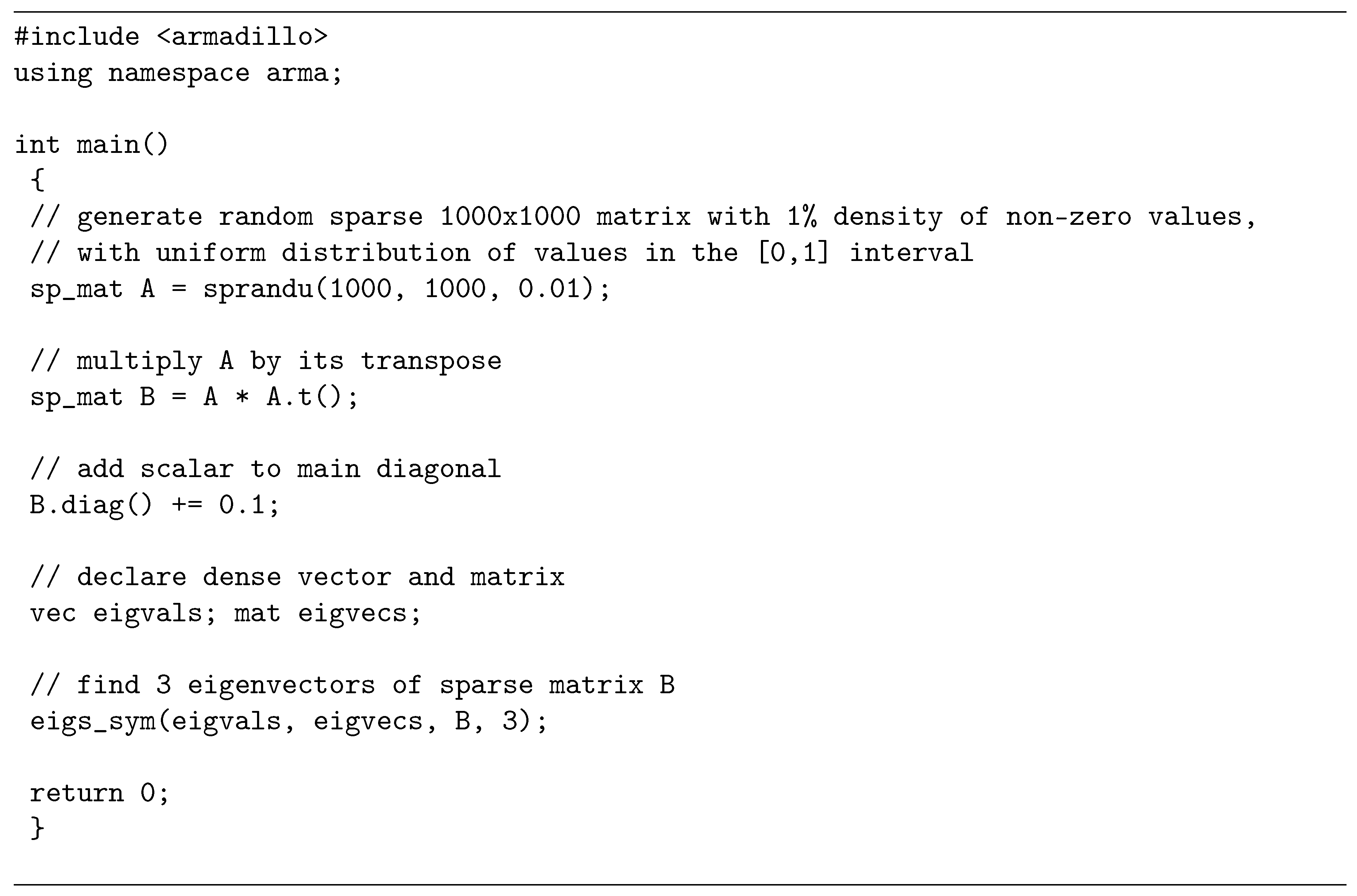
Figure 1 contains a complete C++ program, which briefly demonstrates the usage of the sparse matrix class, while
Table 1 lists a subset of the available functionality.
The aggregate of the sparse matrix class, operator overloading, and associated functions on sparse matrices is an instance of a domain specific language (sparse linear algebra in this case) embedded within the host C++ language [
17,
18]. This allows complex algorithms relying on sparse matrices to be easily developed and integrated within a larger C++ program, making the sparse matrix class directly useful in application/product development.
3. Template-Based Optimisation of Compound Expressions
The sparse matrix class uses a delayed evaluation approach, allowing several operations to be combined to reduce the amount of computation and/or temporary objects. In contrast to brute-force evaluations, delayed evaluation can provide considerable performance improvements, as well as reduced memory usage [
19]. The delayed evaluation machinery is implemented through template meta-programming [
5,
6], where a type-based signature of a compound expression (set of consecutive mathematical operations) is automatically constructed. The C++ compiler is then automatically induced to detect common expression patterns at compile time, followed by selecting the most computationally-efficient implementations.
As an example of the possible efficiency gains, let us consider the expression
trace(A.t() * B), which often appears as a fundamental quantity in semidefinite programs [
20]. These computations are thus used in a wide variety of diverse fields, most notably machine learning [
21,
22,
23]. A brute-force implementation would evaluate the transpose first,
A.t(), and store the result in a temporary matrix
T1. The next operation would be a time-consuming matrix multiplication,
T1 * B, with the result stored in another temporary matrix
T2. The trace operation (sum of diagonal elements) would then be applied on
T2. The explicit transpose, full matrix multiplication and creation of the temporary matrices are suboptimal from an efficiency point of view, as for the trace operation, we require only the diagonal elements of the
A.t() * B expression.
Template-based expression optimisation can avoid the unnecessary operations. Let us declare two lightweight objects, Op and Glue, where Op objects are used for representing unary operations, while Glue objects are used for representing binary operations. The objects are lightweight, as they do not store actual sparse matrix data; instead the objects only store references to matrices and/or other Op and Glue objects. Ternary and more complex operations are represented through combinations of Op and Glue objects. The exact type of each Op and Glue object is automatically inferred from a given mathematical expression through template meta-programming.
In our example, the expression
A.t() is automatically converted to an instance of the lightweight
Op object with the following type:
where
Op<...> indicates that
Op is a template class, with the items between
< and
> specifying template parameters. In this case, the
Op<sp_mat, op_trans> object type indicates that a reference to a matrix is stored and that a transpose operation is requested. In turn, the compound expression
A.t() * B is converted to an instance of the lightweight
Glue object with the following type:
where the
Glue object type in this case indicates that a reference to the preceding
Op object is stored, a reference to a matrix is stored, and a matrix multiplication operation is requested. In other words, when a user writes the expression
trace(A.t() * B), the C++ compiler is induced to represent it internally as
trace(Glue< Op<sp_mat, op_trans>, sp_mat, glue_times>(A,B)).
There are several implemented forms of the
trace() function, one of which is automatically chosen by the C++ compiler to handle the
Glue< Op<sp_mat, op_trans>, sp_mat, glue_times> expression. The specific form of
trace() takes references to the
A and
B matrices, and executes a partial matrix multiplication to obtain only the diagonal elements of the
A.t() * B expression. All of this is accomplished without generating temporary matrices. Furthermore, as the
Glue and
Op objects only hold references, they are in effect optimised away by modern C++ compilers [
6]: the resultant machine code appears as if the
Glue and
Op objects never existed in the first place.
The template-based delayed evaluation approach has also been employed for other functions, such as the diagmat() function, which obtains a diagonal matrix from a given expression. For example, in the expression diagmat(A + B), only the diagonal components of the A + B expression are evaluated.
4. Storage Formats for Sparse Data
We have chosen the three underlying storage formats (CSC, RBT, COO) to give overall efficient execution across several use cases, as well as to minimise the difficulty of implementation and code maintenance burden where possible. Specifically, our focus is on the following main use cases:
Flexible ad-hoc construction and element-wise modification of sparse matrices via unordered insertion of elements, where each new element is inserted at a random location.
Incremental construction of sparse matrices via quasi-ordered insertion of elements, where each new element is inserted at a location that is past all the previous elements according to column-major ordering.
Multiplication of dense vectors with sparse matrices.
Multiplication of two sparse matrices.
Operations involving bulk coordinate transformations, such as flipping matrices column- or row-wise.
The three storage formats, as well as their benefits and limitations, are briefly described below. We use
N to indicate the number of non-zero elements of the matrix, while
n_rows and
n_cols indicate the number of rows and columns, respectively. Examples of the formats are shown in
Figure 2.
4.1. Compressed Sparse Column
The CSC format [
7] uses column-major ordering where the elements are stored column-by-column, with consecutive non-zero elements in each column stored consecutively in memory. Three arrays are used to represent a sparse matrix:
The values array, which is a contiguous array of N floating point numbers holding the non-zero elements.
The rows array, which is a contiguous array of N integers holding the corresponding row indices (i.e., the entry contains the row of the element).
The col_offsets array, which is a contiguous array of n_cols+1 integers holding offsets to the values array, with each offset indicating the start of elements belonging to each column.
Following C++ convention [
2], all arrays use zero-based indexing, i.e., the initial position in each array is denoted by zero. For consistency, element locations within a matrix are also encoded as starting at zero, i.e., the initial row and column are both denoted by zero. Furthermore, the row indices for elements in each column are kept sorted in ascending manner. In many applications, sparse matrices have more non-zero elements than the number of columns, leading to the
col_offsets array being typically much smaller than the
values array.
Let us denote the
entry in the
col_offsets array as
, the
entry in the
rows array as
and the
entry in the
values array as
. The number of non-zero elements in column
i is determined using
, where, by definition,
is always zero and
is equal to
N. If column
i has non-zero elements, then the first element is obtained via
, and
is the corresponding row of the element. An example of this format is shown in
Figure 2b.
The CSC format is well-suited for efficient sparse linear algebra operations such as vector-matrix multiplication. This is due to consecutive non-zero elements in each column being stored next to each other in memory, which allows modern CPUs to speculatively read ahead elements from the main memory into fast cache memory [
24]. The CSC format is also suited for operations that do not change the structure of the matrix, such as element-wise operations on the non-zero elements (e.g., multiplication by a scalar). The format also affords relatively efficient random element access; to locate an element (or determine that it is not stored), a single lookup to the beginning of the desired column can be performed, followed by a binary search [
25] through the
rows array to find the element.
While the CSC format provides a compact representation yielding efficient execution of linear algebra operations, it has two main disadvantages. The first disadvantage is that the design and implementation of efficient algorithms for many sparse matrix operations (such as matrix-matrix multiplication) can be non-trivial [
7,
26]. This stems not only from the sparse nature of the data, but also due to the need to (i) explicitly keep track of the column offsets, (ii) ensure that the row indices for elements in each column are sorted in an ascending manner, and (iii) ensure that any zeros resulting from an operation are not stored. In our experience, designing and implementing new and efficient matrix processing functions directly in the CSC format (which do not have prior publicly available implementations) can be time consuming and prone to subtle bugs.
The second disadvantage of CSC is the computational effort required to insert a new element [
9]. In the worst-case scenario, memory for three new larger-sized arrays (containing the values and locations) must first be allocated, the position of the new element determined within the arrays, data from the old arrays copied to the new arrays, data for the new element placed in the new arrays, and finally, the memory used by the old arrays deallocated. As the number of elements in the matrix grows, the entire process becomes slower.
There are opportunities for some optimisation, such as using oversized storage to reduce memory allocations, where a new element past all the previous elements can be readily inserted. However, this does not help when a new non-zero element is inserted between two existing non-zero elements. It is also possible to perform batch insertions with some speedup by first sorting all the elements to be inserted and then merging with the existing data arrays.
The CSC format was chosen over the related Compressed Sparse Row (CSR) format [
7] for two main reasons: (i) to ensure compatibility with external libraries such as the SuperLU solver [
16] and (ii) to ensure consistency with the surrounding infrastructure provided by the Armadillo library, which uses column-major dense matrix representation to take advantage of low-level functions provided by LAPACK [
27].
4.2. Red-Black Tree
To address the efficiency problems with element insertion at arbitrary locations, we first represent each element as a 2-tuple,
l =
, where
index encodes the location of the element as
. Zero-based indexing is used. This encoding implicitly assumes column-major ordering of the elements. Secondly, rather than using a simple linked list or an array-based representation, the list of the tuples is stored as a Red-Black Tree (RBT), a self-balancing binary search tree [
25].
Briefly, an RBT is a collection of nodes, with each node containing the 2-tuple described above and links to two children nodes. There are two constraints: (i) each link points to a unique child node and (ii) there are no links to the root node. The
index within each 2-tuple is used as the key to identify each node. An example of this structure for a simple sparse matrix is shown in
Figure 2c. The ordering of the nodes and height of the tree (number of node levels below the root node) is controlled so that searching for a specific index (i.e., retrieving an element at a specific location) has a worst-case complexity of
. Insertion and removal of nodes (i.e., matrix elements) also has a worst-case complexity of
. If a node to be inserted is known to have the largest index so far (e.g., during incremental matrix construction), the search for where to place the node can be omitted, which in practice can considerably speed up the insertion process.
With the above element encoding, traversing an RBT in an ordered fashion (from the smallest to largest index) is equivalent to reading the elements in column-major ordering. This in turn allows for quick conversion of matrix data stored in RBT format into CSC format. The location of each element is simply decoded via
= (
) and
=
, where, for clarity,
is the integer version of
z, rounded towards zero. These operations are accomplished via direct integer arithmetic on CPUs. More details on the conversion are given in
Section 5.
Within the hybrid storage framework, the RBT format is used for incremental construction of sparse matrices, either in an ordered or unordered fashion, and a subset of element-wise operations (such as in-place addition of values to specified elements). This in turn enables users to construct sparse matrices in the same way they might construct dense matrices; for instance a loop over elements to be inserted without regard to storage format.
While the RBT format allows for fast element insertion, it is less suited than CSC for efficient linear algebra operations. The CSC format allows for exploitation of fast caches in modern CPUs due to the consecutive storage of non-zero elements in memory [
24]. In contrast, accessing consecutive elements in the RBT format requires traversing the tree (following links from node to node), which in turn entails accessing node data that are not guaranteed to be consecutively stored in memory. Furthermore, obtaining the column and row indices requires explicit decoding of the index stored in each node, rather than a simple lookup in the CSC format.
4.3. Coordinate List Representation
The Coordinate list (COO) is a general concept where a list
L =
of 3-tuples represents the non-zero elements in a matrix. Each 3-tuple contains the location indices and value of the element, i.e.,
l =
. The format does not prescribe any ordering of the elements and a simple linked list [
25] can be used to represent
L. However, in a computational implementation geared towards linear algebra operations [
7],
L is often represented as a set of three arrays:
The values array, which is a contiguous array of N floating point numbers holding the non-zero elements of the matrix.
The rows array, a contiguous array of N integers holding the row index of the corresponding value.
The columns array, a contiguous array of N integers holding the column index of the corresponding value.
As per the CSC format, all arrays use zero-based indexing, i.e., the initial position in each array is zero. The elements in each array are sorted in column-major order for efficient lookup.
The array-based representation of COO is related to CSC, with the main difference that for each element, the column indices are explicitly stored. This leads to the primary advantage of the COO format: it can greatly simplify the implementation of matrix processing algorithms. It also tends to be a natural format many non-expert users expect when first encountering sparse matrices. However, due to the explicit representation of column indices, the COO format contains redundancy and is hence less efficient (space-wise) than CSC for representing sparse matrices. An example of this is shown in
Figure 2d.
To contrast the differences in effort required in implementing matrix processing algorithms in CSC and COO, let us consider the problem of sparse matrix transposition. When using the COO format, this is trivial to implement: simply swap the
rows array with the
columns array, and then, re-sort the elements so that column-major ordering is maintained. However, the same task for the CSC format is considerably more specialised: an efficient implementation in CSC would likely use an approach such as the elaborate TRANSP algorithm by Bank and Douglas [
26], which is described through a 47-line pseudocode algorithm with annotations across two pages of text.
Our initial implementation of sparse matrix transposition used the COO-based approach. COO was used simply due to a shortage of available time for development and the need to flesh out other parts of sparse matrix functionality. When time allowed, we reimplemented sparse matrix transposition to use the above-mentioned TRANSP algorithm. This resulted in considerable speedups, due to no longer requiring the time-consuming sort operation. We verified that the new CSC-based implementation is correct by comparing its output against the previous COO-based implementation on a large set of test matrices.
The relatively straightforward nature of COO format hence makes it well-suited for: (i) functionality contributed by time-constrained and/or non-expert users, (ii) relatively complex and/or less-common sparse matrix operations, and (iii) verifying the correct implementation of algorithms in the more complex CSC format. The volunteer-driven nature of the Armadillo project makes its vibrancy and vitality depend in part on contributions received from users and the maintainability of the code base. The number of core developers is small (i.e., the authors of this paper), and hence, difficult-to-understand or difficult-to-maintain code tends to be avoided, since the resources are simply not available to handle that burden.
The COO format is currently employed for less commonly-used tasks that involve bulk coordinate transformations, such as reverse() for flipping matrices column- or row-wise and repelem(), where a matrix is generated by replicating each element several times from a given matrix. While it is certainly possible to adapt these functions to use the more complex CSC format directly, at the time of writing, we spent our time-constrained efforts on optimising and debugging more commonly-used parts of the sparse matrix class.
5. Automatic Conversion between Storage Formats
To circumvent the problems associated with selection and manual conversion between storage formats, our sparse matrix class employs a hybrid storage framework that automatically and seamlessly switches between the formats described in
Section 4. By default, matrix elements are stored in CSC format. When needed, data in CSC format are internally converted to either the RBT or COO format, on which an operation or set of operations is performed. The matrix is automatically converted (“synced”) back to the CSC format the next time an operation requiring the CSC format is performed.
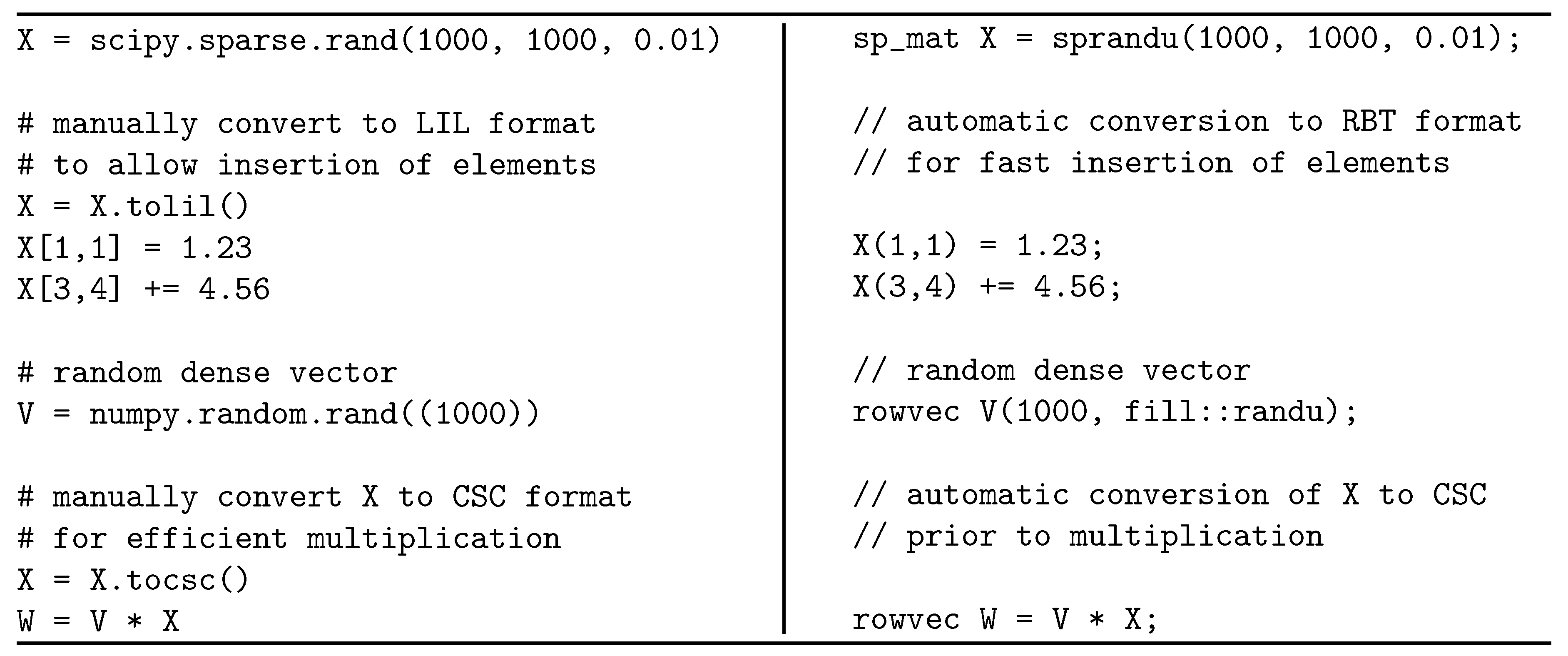
The storage details and conversion operations are completely hidden from the user, who may not necessarily be knowledgeable about (or care to learn about) sparse matrix storage formats. This allows for simplified user code that focuses on high-level algorithm logic, which in turn increases readability and lowers maintenance. In contrast, other toolkits without automatic format conversion can cause either slow execution (as a non-optimal storage format might be used) or require many manual conversions. As an example,
Figure 3 shows a short Python program using the SciPy toolkit [
1] and a corresponding C++ program using the hybrid sparse matrix class. Manually-initiated format conversions are required for efficient execution in the SciPy version; this causes both development time and code required to increase. If the user does not carefully consider the type of their sparse matrix at all times, they are likely to write inefficient code. In contrast, in the C++ program, the format conversion is done automatically and behind the scenes.
A potential drawback of the automatic conversion between formats is the added computational cost. However, it turns out that COO/CSC conversions can be done in a time that is linear in the number of non-zero elements in the matrix and that CSC/RBT conversions can be done at worst in log-linear time. Since most sparse matrix operations are more expensive (e.g., matrix multiplication), the conversion overhead turns out to be mostly negligible in practice. Below, we present straightforward algorithms for conversion and note their asymptotic complexity in terms of the
notation [
25]. This is followed by discussing practical considerations that are not directly taken into account by the
notation.
5.1. Conversion between COO and CSC
Since the COO and CSC formats are quite similar, the conversion algorithms are straightforward. In fact, the only parts of the formats to be converted are the columns and col_offsets arrays with the rows and values arrays remaining unchanged.
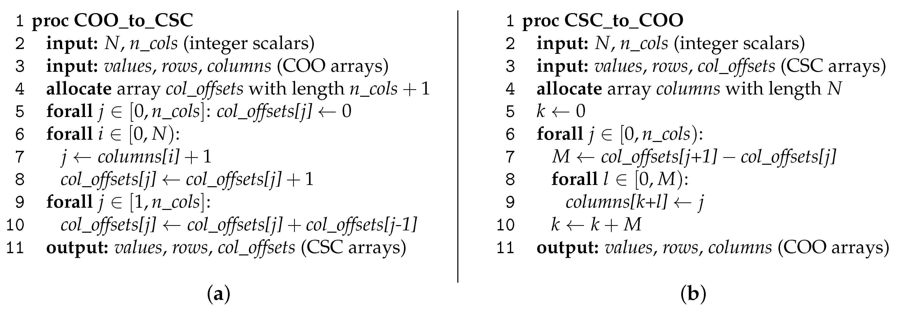
The algorithm for converting COO to CSC is given in
Figure 4a. In summary, the algorithm first determines the number of elements in each column (Lines 6–8), and then ensures that the values in the
col_offsets array are consecutively increasing (Lines 9–10) so that they indicate the starting index of elements belonging to each column within the
values array. The operations listed on Line 5 and Lines 9–10 each have a complexity of approximately
, while the operation listed on Lines 6–8 has a complexity of
, where
N is the number of non-zero elements in the matrix and
n_cols is the number of columns. The complexity is hence
. As in most applications, the number of non-zero elements will be considerably greater than the number of columns; the overall asymptotic complexity in these cases is
.
The corresponding algorithm for converting CSC to COO is shown in
Figure 4b. In essence, the
col_offsets array is unpacked into a
columns array with length
N. As such, the asymptotic complexity of this operation is
.
5.2. Conversion between CSC and RBT
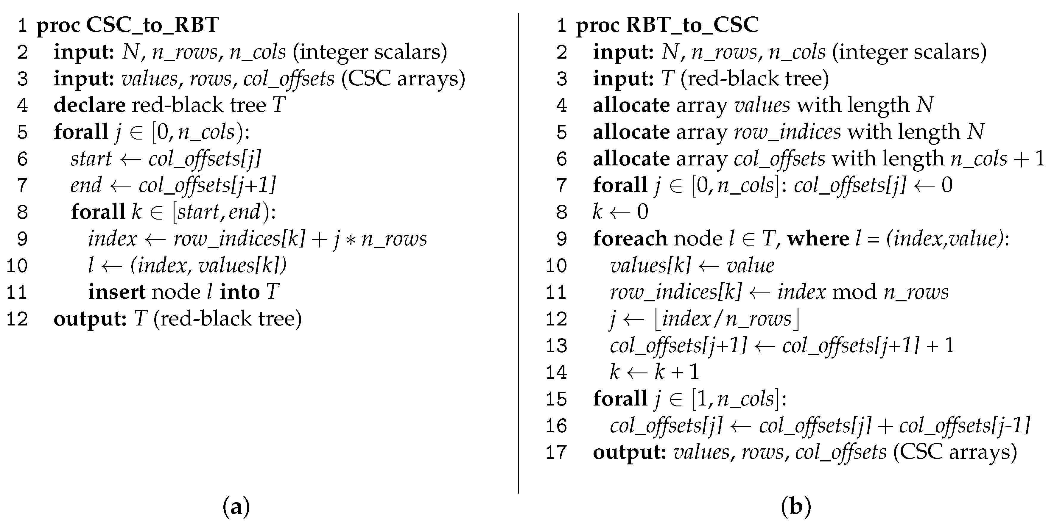
The conversion between the CSC and RBT formats is also straightforward and can be accomplished using the algorithms shown in
Figure 5. In essence, the CSC to RBT conversion involves encoding the location of each matrix element to a linear index, followed by inserting a node with that index and the corresponding element value into the RBT. The worst-case complexity for inserting all elements into an RBT is
. However, as the elements in the CSC format are guaranteed to be stored according to column-major ordering (as per
Section 4.1) and the location encoding assumes column-major ordering (as per
Section 4.2), the insertion of a node into an RBT can be accomplished without searching for the node location. While the worst-case cost of
is maintained due to tree maintenance (i.e., controlling the height of the tree) [
25], in practice, the amortised insertion cost is typically lower due to the avoidance of the search.
Converting an RBT to CSC involves traversing through the nodes of the tree from the lowest to highest index, which is equivalent to reading the elements in column-major format. The value stored in each node is hence simply copied into the corresponding location in the CSC
values array. The index stored in each node is decoded into row and column indices, as per
Section 4.2, with the CSC
row_indices and
col_offsets arrays adjusted accordingly. The worst-case cost for finding each element in the RBT is
, which results in the asymptotic worst-case cost of
for the whole conversion. However, in practice, most consecutive elements are in nearby nodes, which on average reduces the number of traversals across nodes, resulting in considerably lower amortised conversion cost.
5.3. Practical Considerations
Since the conversion algorithms given in
Figure 4 and
Figure 5 are quite straightforward, the
notation does not hide any large constant factors. For COO/CSC conversions, the cost is
, while for CSC/RBT conversions, the worst-case cost is
. In contrast, many mathematical operations on sparse matrices have much higher computational cost than the conversion algorithms. Even simply adding two sparse matrices can be much more expensive than a conversion. Although the addition operation still takes
time (assuming
N is identical for both matrices), there is much hidden constant overhead, since the sparsity pattern of the resulting matrix must be computed first [
7]. A similar situation applies for multiplication of two sparse matrices, whose cost is in general superlinear in the number of non-zeros of either input matrix [
26,
28]. Sparse matrix factorisations, such as LU factorisation [
16,
29] and Cholesky factorisation [
30], are also much more expensive than the conversion overhead. Other factorisations and higher level operations can exhibit similar complexity characteristics. Given this, the cost of format conversions is heavily outweighed by the user convenience that they allow.
6. Empirical Evaluation
To demonstrate the advantages of the hybrid storage framework and the template-based expression optimisation mechanism, we performed a set of experiments, measuring the wall-clock time (elapsed real time) required for:
Unordered element insertion into a sparse matrix, where the elements are inserted at random locations in random order.
Quasi-ordered element insertion into a sparse matrix, where each new inserted element is at a random location that is past the previously inserted element, under the constraint of column-major ordering.
Calculation of , where A and B are randomly-generated sparse matrices.
Obtaining a diagonal matrix from the expression, where A and B are randomly-generated sparse matrices.
In all cases, the sparse matrices had a size of 10,000 × 10,000, with four settings for the density of non-zero elements: 0.01%, 0.1%, 1%, and 10%. The experiments were done on a machine with an Intel Xeon E5-2630L CPU running at 2 GHz, using the GCC v5.4 compiler. Each experiment was repeated 10 times, and the average wall-clock time is reported. The wall-clock time measured the total time taken from the start to the end of each run and included necessary overheads such as memory allocation.
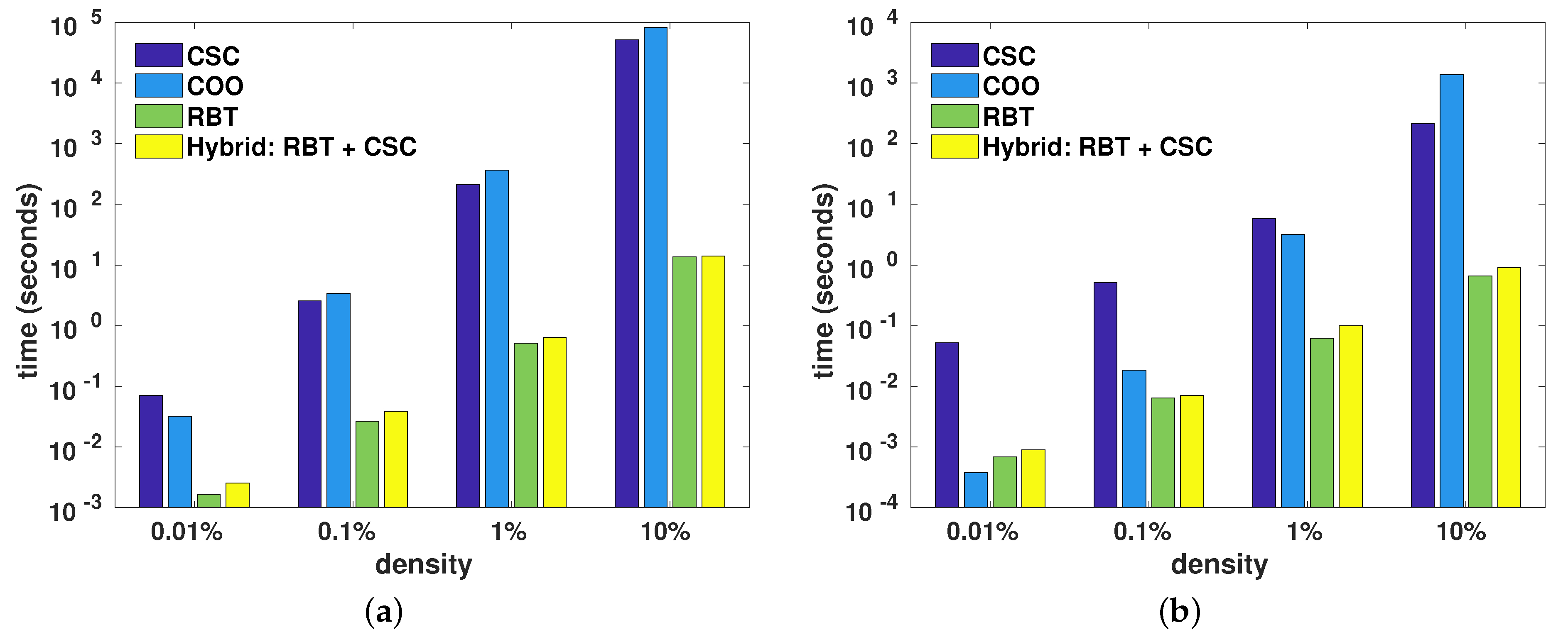
Figure 6 shows the average wall-clock time taken for element insertion done directly using the underlying storage formats (i.e., CSC, COO, and RBT, as per
Section 4), as well as the hybrid approach, which used RBT followed by conversion to CSC. The CSC and COO formats used oversized storage as a form of optimisation (as mentioned in
Section 4.1), where the underlying arrays were grown in chunks of 1024 elements in order to reduce both the number of memory reallocations and array copy operations due to element insertions.
In all cases bar one, the RBT format was the quickest for insertion, generally by one or two orders of magnitude. The conversion from RBT to CSC added negligible overhead. For the single case of quasi-ordered insertion to reach the density of 0.01%, the COO format was slightly quicker than RBT. This was due to the relatively simple nature of the COO format, as well as the ordered nature of the element insertion where the elements were directly placed into the oversized COO arrays (i.e., no sorting required). Furthermore, due to the very low density of non-zero elements and the chunked nature of COO array growth, the number of reallocations of the COO arrays was relatively low. In contrast, inserting a new element into RBT required the allocation of memory for a new node and modifying the tree to append the node. For larger densities (), the COO element insertion process quickly became more time consuming than RBT element insertion, due to an increased amount of array reallocations and the increased size of the copied arrays. Compared to COO, the CSC format is more complex and has the additional burden of recalculating the column offsets (col_offsets) array for each inserted element.
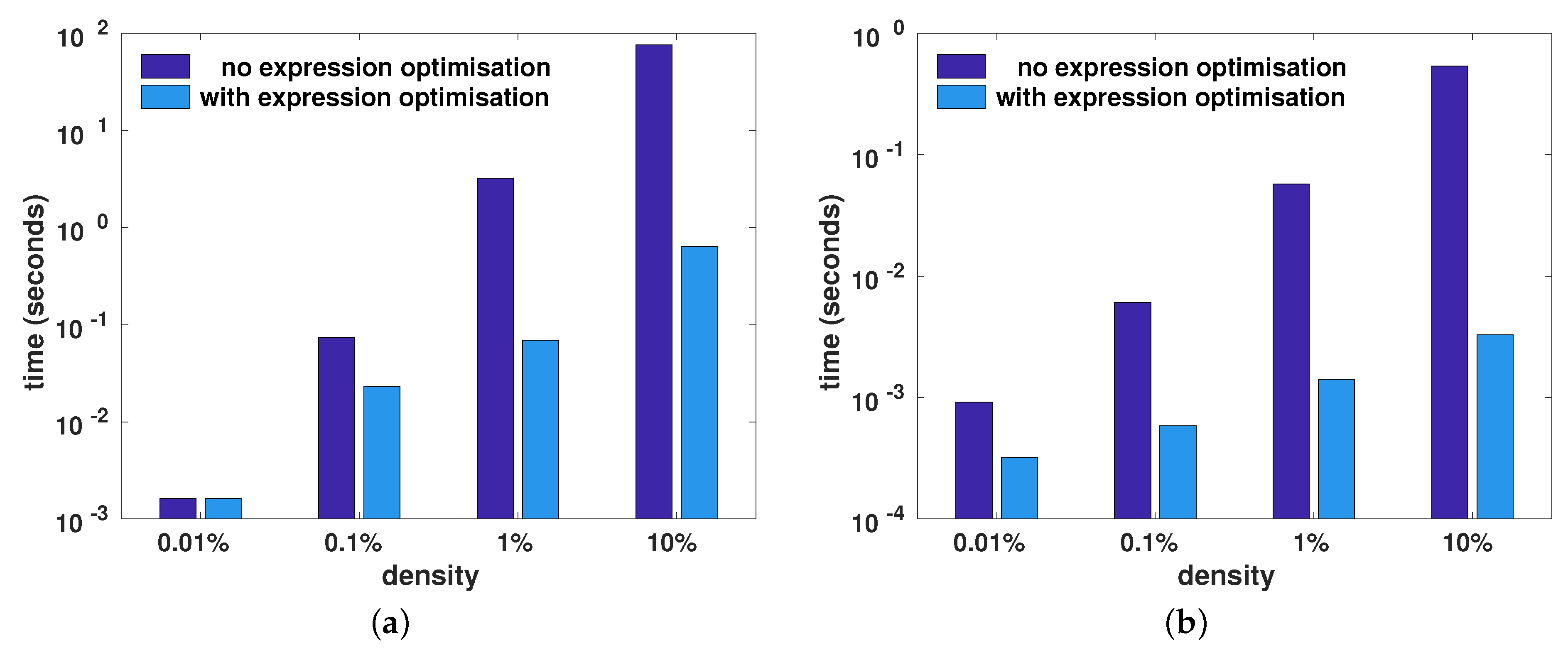
Figure 7 shows the wall-clock time taken to calculate the expressions
trace(A.t()*B) and
diagmat(A+B), with and without the aid of the automatic template-based optimisation of compound expression described in
Section 3. For both expressions, employing expression optimisation led to considerable reduction in the wall-clock time. As the density increased (i.e., more non-zero elements), more time was saved via expression optimisation.
For the trace(A.t()*B) expression, the expression optimisation computed the trace by omitting the explicit transpose operation and performing a partial matrix multiplication to obtain only the diagonal elements. In a similar fashion, the expression optimisation for the diagmat(A+B) expression directly generated the diagonal matrix by performing a partial matrix addition, where only the diagonal elements of the two matrices were added. As well as avoiding full matrix addition, the generation of a temporary intermediary matrix to hold the complete result of the matrix addition was also avoided.
7. Conclusions
Driven by a scarcity of easy-to-use tools for algorithm development that requires the use of sparse matrices, we devised a practical sparse matrix class for the C++ language. The sparse matrix class internally uses a hybrid storage framework, which automatically and seamlessly switches between several underlying formats, depending on which format is best suited and/or available for specific operations. This allows the users to write sparse linear algebra without requiring them to consider the intricacies and limitations of various storage formats. Furthermore, the sparse matrix class employs a template meta-programming framework that can automatically optimise several common expression patterns, resulting in faster execution.
The source code for the sparse matrix class and its associated functions is included in recent releases of the cross-platform and open-source Armadillo linear algebra library [
3], available from
http://arma.sourceforge.net. The code is provided under the permissive Apache 2.0 license [
31], allowing unencumbered use in both open-source and proprietary projects (e.g., product development).
The sparse matrix class has already been successfully used in open-source projects such as the mlpack library for machine learning [
32], and the ensmallen library for mathematical function optimisation [
33]. In both cases, the sparse matrix class is used to allow various algorithms to be run on either sparse or dense datasets. Furthermore, bi-directional bindings for the class are provided to the R environment via the Rcpp bridge [
34]. Avenues for further exploration include expanding the hybrid storage framework with more sparse matrix formats [
7,
12,
13] in order to provide speedups for specialised use cases.


