Influence of a Modulated Parameter on Hantavirus Infection

Abstract

We study the dynamical behavior of a model commonly used to describe the infection of mice due to hantavirus (and, therefore, its possibility of propagation into human populations) when a parameter is changed in time. In particular, we study the situation when the ecological conditions (e.g., climate benignity, food availability, and so on) change periodically in time. We show that the density of infected mice increases abruptly as the parameter crosses a critical value. We correlate such a situation with the observed sudden outbreaks of hantavirus. Finally, we discuss the possibility of preventing a hantavirus epidemic.

1. Introduction

The mouse colilargo (Oligoryzomis longicaudatus), unlike the other group of rodents present in South America since the arrival of Europeans, does not hibernate. Thus, it devotes all its leisure time to the intensive proliferation of its species. The colilargo is indicated as a carrier of the Hanta “Andes” virus, the strain of hantavirus that is found in the Andean–Patagonian zone. Numerous observations [1,2,3] carried out in several areas have shown a marked increase in the population of this rodent when there are positive ecological conditions (e.g., climate benignity and increased food availability). In this case, population explosions of these so-called “rats” may occur. The population of rodents increases notoriously because these sub-species respond quickly to the supply of food and to benevolent climate conditions. In some cases, the population density of colilargo (with normal values of 10 to 100 individuals per hectare) can rise to about 1000 to 1500 individuals per hectare [4,5]. This overpopulation generates stress among the mice, due to agglomeration and competition for food, which makes them more aggressive, generating many fights with bite wounds, which increases the propagation of the hantavirus. This behavior has been cited as the reason explaining the significant correlation between the index of abundance and the number of positive animals detected. The proportion of seropositivity can increase from 5% up to 10% of the total population of the mice [5]. High population densities also lead them to propagate outwards in space, looking for food or just better living conditions. Different types of rodents transmit the hantavirus in the different geographic areas of the world, and all must be considered potentially dangerous. Hantavirus, although with a low probability of infection, is not unimpressive in terms of its mortality. The mortality rate for humans is around 40% and it has not been possible to obtain a successful vaccine for this disease thus far [5]. Therefore, a good knowledge on the dynamics of the colilargo population could help to predict changes in the risks of human hantavirus infection and generate prevention policies. A mathematical model has already been proposed to analyze the propagation of hantavirus [6,7]. The model was based on the population dynamics of the mice and studied the evolution of the populations of healthy and infected mice. in [6], a study of spatial effects through the diffusion of mice (i.e., diffusion mainly characterized their movement through space) was carried out; additionally, a random variation of a parameter was included. In [8], the authors showed that the inclusion of the movement of the mice with respect to space (i.e., the diffusion term) affected additional features of the simulation in a physically understandable manner, with higher diffusion constants leading to greater agreement with the mean field results. Here, we show, instead, that diffusion is not necessary in order to explain a sudden increase in the density of infected mice and, as a consequence, the appearance of an epidemic of hantavirus. As the influence of the environmental conditions play a role in the evolution of the population, both at the seasonal level and at the level of very long cycles, we propose a model taking into account a variable parameter to analyze the population dynamics of the colilargo mice. We analyze the dynamical solutions and we show how the number of infected mice increases abruptly when a threshold of the control parameter is crossed. Such an increase may generate a large expansion in the transmission of the disease, even without the existence of diffusion.

2. Model and Results

If we take into account only the temporal evolution of the susceptible $M_s$ and infected $M_i$ mice, the corresponding differential equations (as introduced in [6,7]) are:

$$\left\{\begin{array}{c}\frac{d{M}_s}{dt}=(b-c)M_s+b{M}_i-(a+\frac{1}{K})M_s{M}_i-\frac{1}{K}{M}_s^2\hfill \\ \frac{d{M}_i}{dt}=-c{M}_i+(a-\frac{1}{K})M_s{M}_i-\frac{1}{K}{M}_i^2\hfill \end{array}\right.,$$

(1)

where the parameters b and c are the natural rates of birth and death of the susceptible and infected mice, respectively; a is the infection rate of the susceptible mice that become infected due to an encounter with an infected mouse; and the parameter K, in both equations, takes into account the limitations in the process of population growth due to competition for shared resources, which called the carrying capacity and is defined, for each biological species, as the maximum population size of the species that the environment can sustain indefinitely, in accordance with their necessities. It is well-known that the infection is chronic: Infected mice do not die of it, and they do not lose their infectiousness (probably for their whole life). Therefore, the rate c is the same for both categories of mice. It is worthwhile to note that all mice are born susceptible at a rate proportional to the total number of mice, since all mice contribute equally to procreation. Even if these equations allow for a simple interpretation of each term, it is convenient to write them in terms of the total number of mice $M=M_s+M_i$ and the infected mice $M_i$. By just adding the two differential equations above and replacing $M_s$ in terms of M and $M_i$, we get:

$$\left\{\begin{array}{c}\frac{dM}{dt}=(b-c)M-\frac{1}{K}{M}^2=F(M,M_i)\hfill \\ \frac{d{M}_i}{dt}=-c{M}_i+(a-\frac{1}{K})M{M}_i-a{M}_i^2=G(M,M_i)\hfill \end{array}\right..$$

(2)

If the variable M is independent of $M_i$, then it is trivial to find the stationary solutions and their stability.

The total number of mice takes only two steady-state values:

$$\begin{array}{c}M=0\hfill \\ \mathrm{and}M=K(b-c).\hfill \end{array}$$

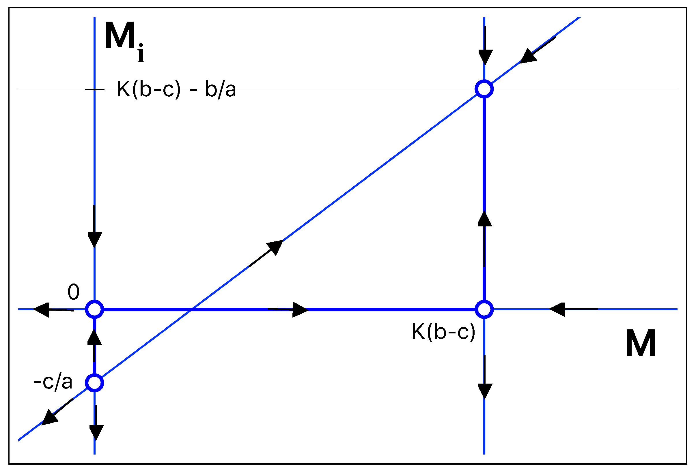
The first one indicates that such a type of mouse does not exist in the region and the second one is proportional to the difference between birth and death rates, where the constant of proportionality is the carrying capacity. In a phase space portrait, the two straight lines corresponding to the possible values of M are two of the nullclines (zero-growth isoclines) of the dynamical system. The equation corresponding to the infected mice immediately gives the following nullclines:

$$\begin{array}{c}{M}_i=0,\mathrm{and}\hfill \\ M_i=(a-\frac{1}{K})M-c.\hfill \end{array}$$

The four nullclines are represented in Figure 1 in the space of $M_i$ as a function of M. Their intersections are the fixed points of the system:

$$\begin{array}{c}{(M,M_i)}_1=(0,0)\hfill \\ {(M,M_i)}_2=(0,\frac{-c}{a})\hfill \\ {(M,M_i)}_3=(K(b-c),0)\hfill \\ {(M,M_i)}_4=(K(b-c),K(b-c)-\frac{b}{a})\hfill \end{array}.$$

The first steady-state solution is the trivial one, in which there are no mice in the region of interest. The second steady-state solution, ${(M,M_i)}_2$ = $(0,\frac{-c}{a})$, is not compatible with the problem as the number of infected mice is negative. The third and the fourth solutions are interesting solutions. The third solution corresponds to a situation in which all mice are healthy, and the number of infected mice vanishes. For the solution ${(M,M_i)}_4$ = $(K(b-c),K(b-c)-\frac{b}{a})$ susceptible and infected mice co-exist, with $M_s$ = $\frac{b}{a}$.

A very simple linear stability analysis gives the region in parameter space where one of the solutions will prevail. The Jacobian $\mathsf{\Gamma }$ of the system is:

$$\begin{array}{c}\hfill \mathsf{\Gamma }=\left[\begin{array}{cc}{\partial }_{M}F(M,M_i)& {\partial }_{M_i}F(M,M_i)\\ {\partial }_{M}G(M,M_i)& {\partial }_{M_i}G(M,M_i)\end{array}\right]=\left[\begin{array}{cc}(b-c)-2\frac{1}{K}M& 0\\ (a-\frac{1}{K})M& -c+(a-\frac{1}{K})M-2a{M}_i\end{array}\right]\end{array}.$$

Then, the eigenvalues of $\mathsf{\Gamma }$ corresponding to the $(0,0)$ solution are:

$$\begin{array}{c}{\lambda }_1=b-c\hfill \\ \mathrm{and}{\lambda }_2=-c\hfill \end{array}.$$

Thus, as expected, the trivial solution is stable if the death rate is bigger than the birth rate, which causes the extinction of the mice. If the birth rate is greater than the death rate, the solution is clearly a saddle point. The eigenvalues for the $(K(b-c),0)$ solution are:

$$\begin{array}{c}{\lambda }_1=-(b-c)\hfill \\ \mathrm{and}{\lambda }_2=Ka(b-c)-b\hfill \end{array}.$$

This solution will be stable if the birth rate b remains in the range:

$$c<b<c/(1-(1/Ka)).$$

For values of the $Ka$ product greater than one, there exists a range of the birth rates for which the solution with all mice healthy is stable. It is important to notice that the upper limit depends on the value of K, and that the range of stability is reduced for large values of K. Outside the range of stability, the solution becomes a saddle point. Finally, the stationary solution $(K(b-c),K(b-c)-\frac{b}{a})$, which predicts the co-existence of healthy and infected mice, is stable if $b>c/(1-(1/Ka))$. At a fixed value of the birth rate $b>c$, there exists a critical value of K at which there is an exchange of stability between the last two steady-state solutions. At that point, we have a transcritical bifurcation, leading to the appearance of infected mice. The critical value of the carrying capacity $K_c$ is given by:

$$K_c=b/[a(b-c)].$$

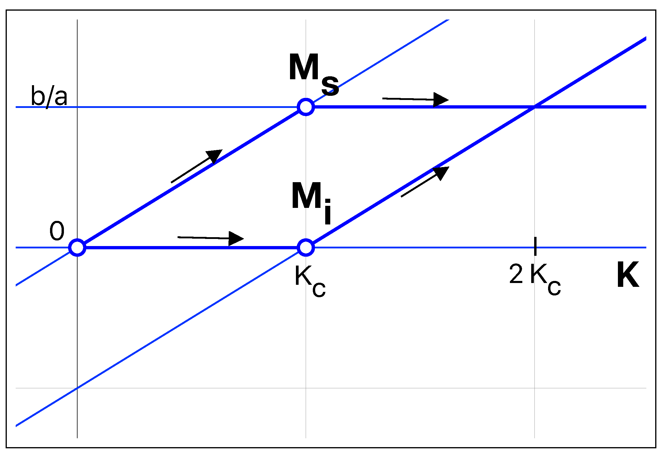
We show the two relevant stationary solutions as a function of K for a birth rate bigger than the death rate in Figure 2. The bifurcation happens at the exact point where the number of infected mice becomes positive. Above the bifurcation point, the number of infected mice is proportional to the carrying capacity. 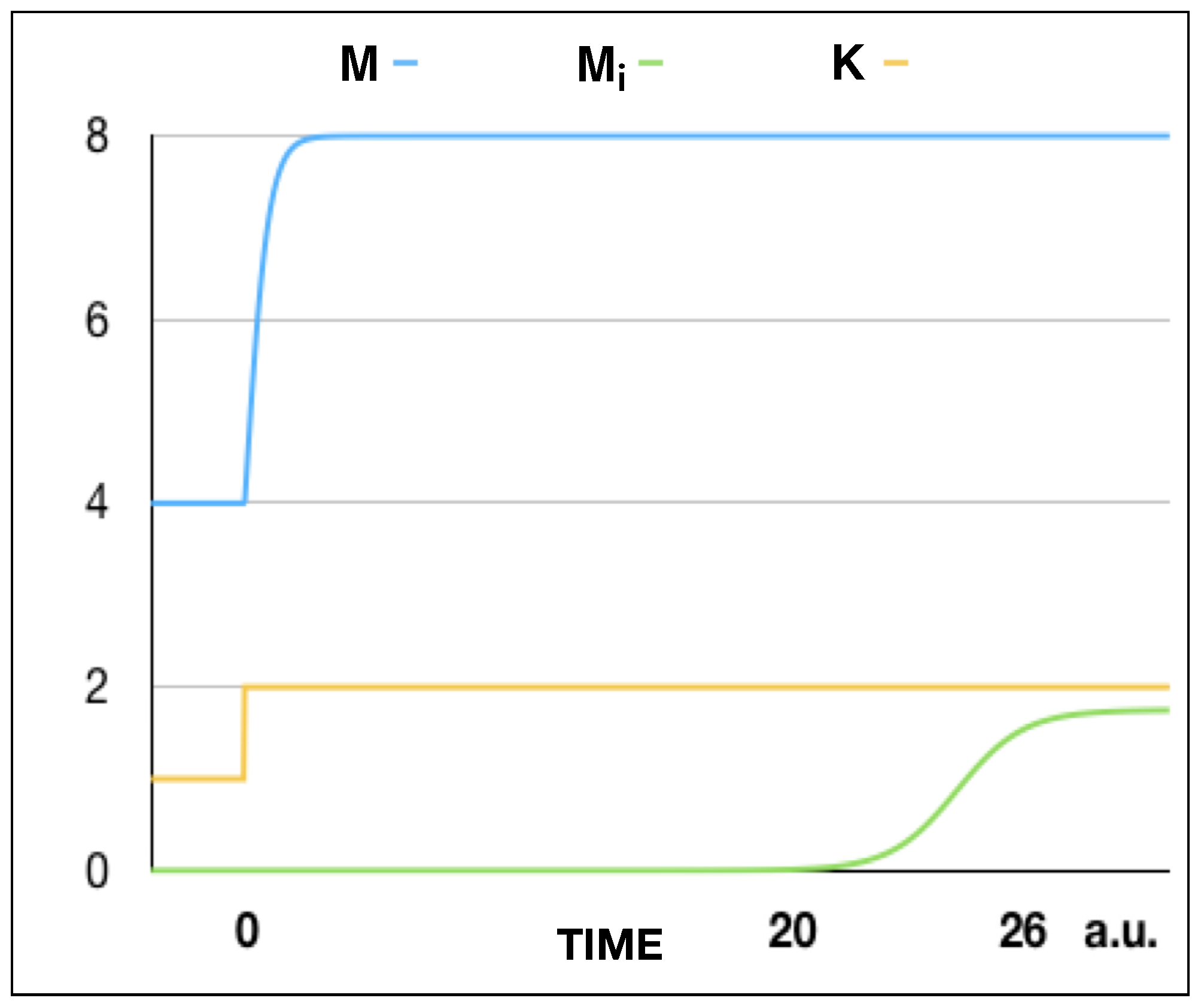The transcritical bifurcation is a smooth transformation and, therefore, it predicts a relatively slow increase in the number of infected mice as the carrying capacity K is swept across the critical value. As stated above, the mouse colilargo does not hibernate; thus, we can consider the birth rate, as well as the death rate, to be almost constant in time. We will assume, also, that the the rate of infection per mouse (a) is constant. If the capacity K is suddenly increased from an initial value $K_{init}$ below the threshold to a final value $K_{fin}$ above the threshold, the total number of mice increases relatively fast, from the stationary solution corresponding to $K_{init}$ towards the steady-state solution corresponding to the final value of K. The number of infected mice will increase from 0 to the steady-state value with a well-marked lethargy, as can be seen in Figure 3. The bifurcation delay is a well-known effect each time a parameter is swept across a bifurcation point [9,10], which is a consequence of the critical slowing down at the bifurcation point [11]. The delay time measured when the parameter changes discontinuously corresponds to the minimum delay. As long as the speed at which the parameter changes decreases, the delay time increases.

Here, we analyze the behavior of the dynamical system when the the carrying capacity K changes relatively slowly, compared to the characteristic time of the variables. We introduce the following temporal variation of the carrying capacity:

$$K=K_0(1+mcos(\omega t)).$$

(3)

Even if a periodic and smooth modulation of the carrying capacity does not strictly adhere to reality, it allows us to understand the origins of the different possible dynamical behaviors and, therefore, to correlate them to the real observations. In order to make the simulation realistic, we would need to introduce a noise term on the temporal evolution of the carrying capacity, because it is affected by several external factors which change from season to season. However, it is not the objective of this manuscript to compare numerical results with quantitative data, but, instead, to understand the qualitative processes in the dynamics of mouse populations. We analyze three different situations corresponding to different values of $K_0$ and m. In the first one, $K_0$ is smaller than $K_c$ and m is such that the maximum value of K is still smaller than $K_c$. In the second one, $K_0$ is greater than $K_c$ and the minimum value of K is still larger than $K_c$. Finally, the third is a situation in which K is swept across the critical value. In the first case, the number of healthy mice is modulated while the number of infected mice vanishes independently of the initial condition. During the whole modulation period, the solution with no infected mice remains stable. 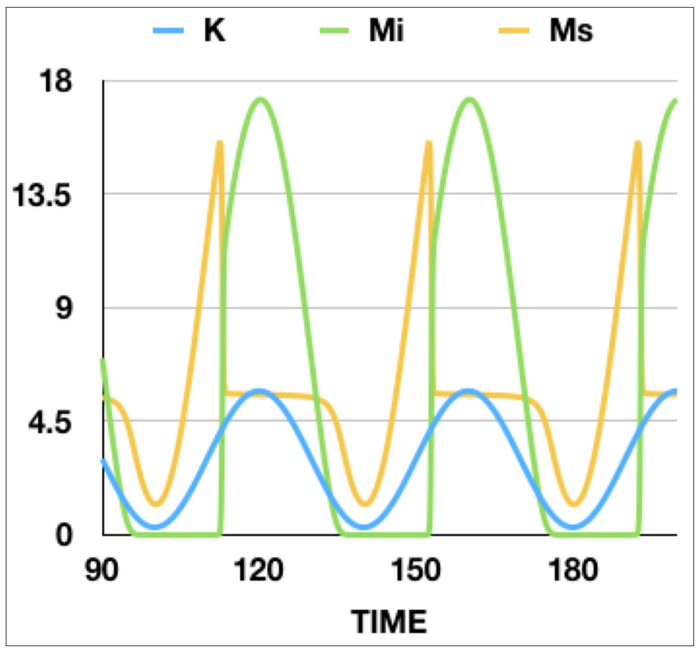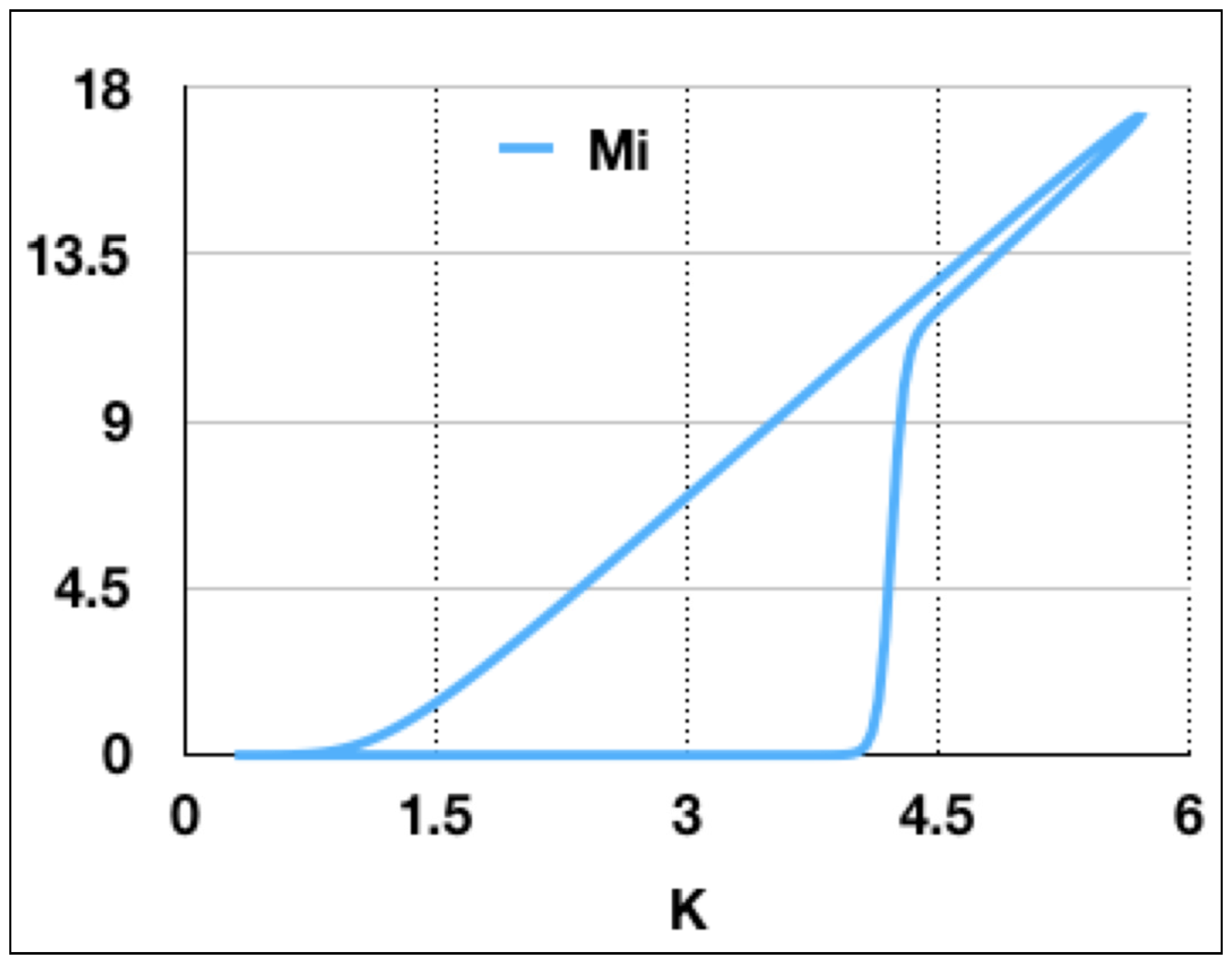In this case, a seed of infected mice will vanish independently of the value of K. In the second case, there is always a positive number of infected mice, which becomes modulated as well as the total population of mice. The modulation follows the modulation of the carrying capacity with a different phase. The last case is the most interesting one, because the carrying capacity is swept across the bifurcation point and the system has to switch between the two solutions (which are alternating their stabilities). In this paper, we analyze the behavior of the number of mice when the frequency of the modulated parameter is smaller than the response rate of the variables. It is worthwhile to note that the frequency of the modulation, together with the amplitude of the modulation, will define the average speed at which the parameter is changed; thus, they will determine the delay time in the bifurcation. The most noticeable result consists of the fact that the number of infected mice will not increase continuously from 0 to a value that will follow the modulation. In fact, by simple observation of Figure 4, it is clear that, at a certain value of K, the number of infected mice will grow discontinuously. This behavior is more appropriate of a saddle-type bifurcation than a transcritical bifurcation. As a consequence, the number of susceptible mice $M_s$ decreases abruptly while, at the same time, the number of infected mice $M_i$ increases. It is evident that a graph of $M_i$ as a function of K will show a bistable behavior as K swept across the bifurcation up and down (Figure 5). It is important to remark that the bistable behavior is a dynamical one. If the sweeping is stopped at any moment, the system will evolve towards the corresponding stable steady-state solution.

It is important to notice that this type of dynamical behavior is general and is a simple consequence of the critical slowing down at the bifurcation point. It happens by modulating every parameter and appears in a very large range of frequencies and amplitudes of the modulation, because it is intrinsically associated to the existence of a bifurcation point. The behavior will be different only if the modulation period is smaller than the decay time of the variable. A simple analysis of Figure 4 allows us to conclude that, in this simple model, a sudden increase in the infected mice is a consequence of the sweeping of a control parameter across a bifurcation point. Thus, the variable $M_i$ does not adiabatically follow the change of the parameter, even if the rate of change of the parameter is slower than the response rate of the variable. It is worthwhile to notice that, once the number of infected mice switches on, the number of susceptible mice remains constant and the dynamical system adiabatically follows the increase of the capacity by increasing the number of infected mice. During the time that K is decreasing, the system follows almost adiabatically the evolution of the parameter, with a very small delay. The consequence of this delay is that the number of infected mice vanishes at values of K slightly smaller than the one corresponding to the bifurcation point.

3. Discussion

The results shown above suggest that the capacity K may control the appearance and disappearance of hantavirus infection in rats. In fact, if K is always below $K_c$, only susceptible mice exist. If just a few mice get infected, this perturbation will decay faster towards the situation where infected mice vanish. If K is always above the critical value, then infected mice will always exist. If the capacity oscillates around the $Kc$ value, then the variables $M_i$ and $M_s$ do not adiabatically follow the change in K. The delayed bifurcation generates an almost discontinuous increase of the infected mice and, therefore, this effect can be understood as the origin of an outbreak of hantavirus infection among the mice with the consequence of an epidemic among other living mammals and, in particular, humans beings. On the other hand, the delay in the bifurcation justifies the infection disappearing for long periods of time, even if the carrying capacity is already above the critical value $K_c$; however, a further increase in K will trigger a almost immediate epidemic in the population of mice. Furthermore, it is necessary to reduce K below the critical value $K_c$ in order to be able to eradicate the disease again. Finally, we re-affirm the importance of the non-intuitive concept that slow variations of some ecological parameters can trigger an outbreak of hantavirus infection. This concept should be taken into account in the development of public health policies.

4. Conclusions

In conclusion, we propose that a typical ecological model representing the temporal evolution of mouse population densities can explain several aspects of the propagation of hantavirus. A relatively fast variation of the parameters controlling the carrier capacity K, or of any of the parameters of the system, will produce continuous variations in their densities and a continuous, but predictable, increase in infection. However, a changing parameter which varies much slower may cause a much faster increase in the density of infected mice, generating an epidemic of hantavirus in mice. The ideal situation is represented by the situation in which the environmental conditions maintain the system below the threshold of the transcritical bifurcation. In this situation, the density of infected mice can not grow and it will always decay to a vanishing quantity. In this paper, we studied the effects of a slow variation of the environmental conditions for the mice. As a future work, it will be necessary to take into account the situations in which the living conditions change very quickly, compared to the response time of the system, and also the transmission of hantavirus among human beings.