Analysis of a Model of Leishmaniasis with Multiple Time Lags in All Populations

Abstract

There are several types of deterministic compartmental models for disease epidemiology such as SIR, SIS, SEIS, SEIR, etc. The exposed population group in, for example SEIS or SEIR, usually represents individuals in the incubation class. Time delays (of which there are several types) when incorporated into a SIR or SIS model, also fulfil the role of the incubation period without necessarily adding another compartment to the model. This paper incorporates time delays into a SIS model that describes the transmission dynamics of cutaneous leishmaniasis. The time lags account for the incubation periods within the sandflies vector, the human hosts and the different animal groups that serve as reservoir hosts. A threshold value, $R_0$, of the model is computed and used to study the disease-free equilibrium and endemic equilibrium of the system. Analysis demonstrating local and global stability of the disease-free equilibrium when $R_0<1$ is provided for all $n+1$ population groups involved is provided. The existence of an endemic equilibrium is only guaranteed when $R_0>1$ and numerical analysis of the endemic equilibrium for a human host, a vector host and a single animal reservoir host that is globally stable is also provided.

1. Introduction

Leishmaniasis is primarily a zoonotic disease caused by protozoan parasites that are transmitted to humans by female sandflies. Animals including dogs, cattle, rodents and many others are the main reservoir of the parasite and occasionally humans in some localities. About 30 different species of sandflies are known to transmit more than 20 species of Leishmania parasites resulting in human infection. The incubation period within humans and animals range from two to eight weeks, while that in the sandflies range from four to 25 days [1]. Several forms of the disease have been identified, with the main types being cutaneous, visceral, and mucocutaneous leishmaniasis. Cutaneous leishmaniasis (CL) is the most dominant form of the disease leading to skin lesions that can lead to lifelong scars and disabilities. Visceral leishmaniasis is the most fatal, causing enlargement of the spleen and liver, while mucocutaneous leishmaniasis affects mostly the mucous membranes of the nose and mouth, destroying them in the process.

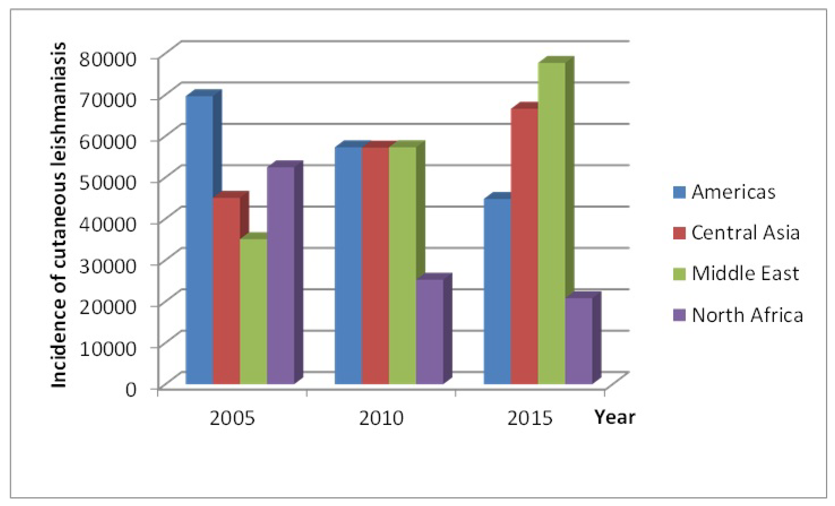
There is currently no vaccine for CL and although the disease can be treated, the majority of cases occur in developing countries. Estimates of new cases of CL per year range from about $700,000$ to 1.2 million or more worldwide [2]. 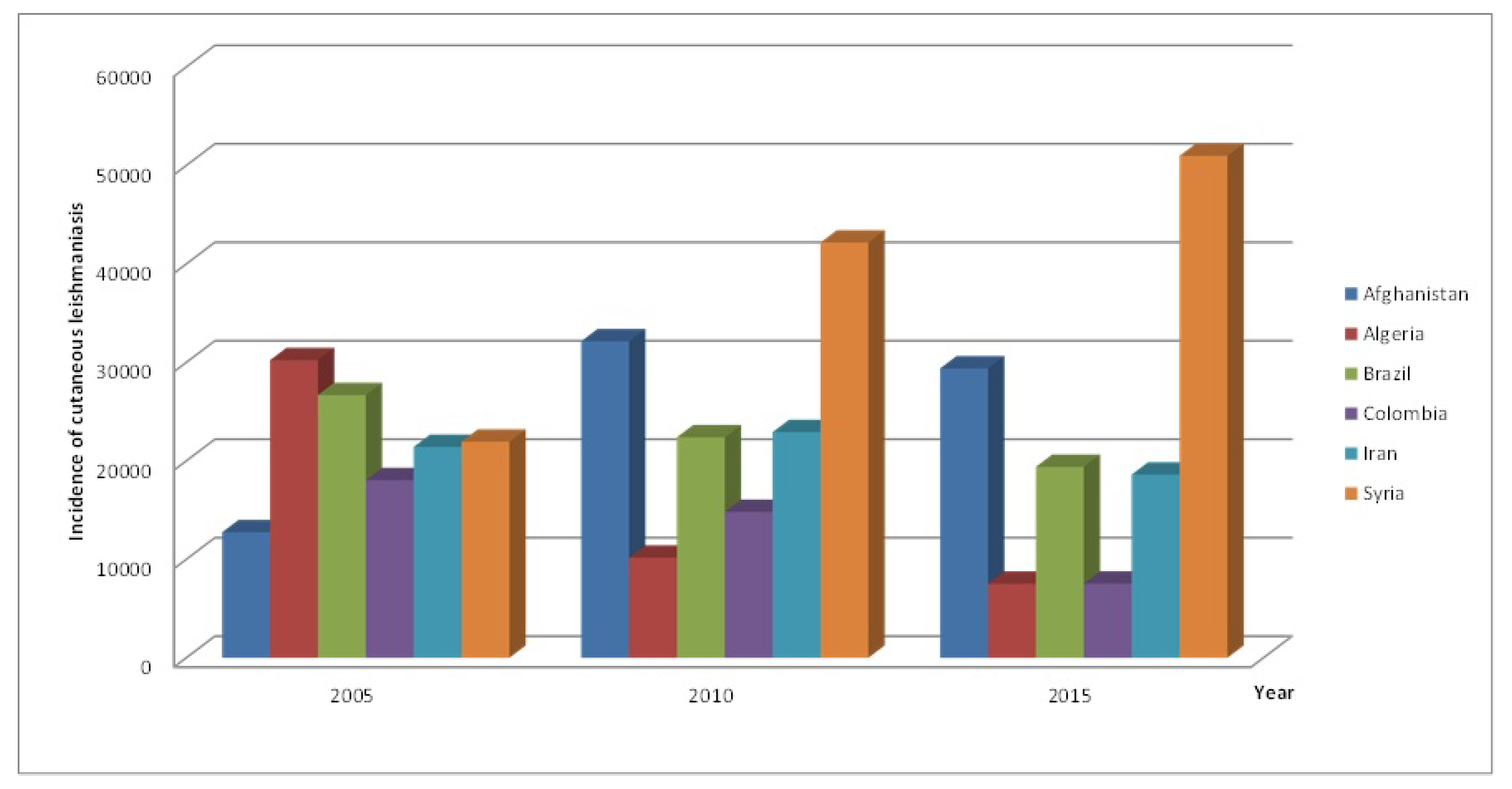In recent years, CL has become increasingly prevalent in urban areas of Latin America, north Africa and central Asia and the Middle East, with these regions contributing about $95\%$ of new CL cases annually (see Figure 1). Within the endemic regions, six countries, namely; Afghanistan, Algeria, Brazil, Colombia, Iran and Syria, accounted for more than two thirds of new CL cases in 2015 (see Figure 2) [3]. Symptoms of CL in humans are primarily ulcerated lesions on the skin that can take anywhere between a few months and a few years to heal, though cases lasting longer than a year are rare. The lesions usually leave depressed scars on the skin, and can have debilitating effects depending on where they occur. Treatment when available can hasten the healing of lesions and prevents spreading to other parts of the body. Although recognized as one of the most important and widespread parasitic disease in the world, CL prevention and control remains a challenge for health authorities in some countries [4].

Mathematical modeling and analysis has been at the center of infectious disease epidemiology since the classical works of Ross [5] and Macdonald [6]. Various forms of compartmental models for infectious diseases have been formulated [7]. Several models studying the transmission dynamics of CL have been proposed [8,9,10,11,12,13,14]. See [15,16] for a review of mathematical models for visceral leishmaniasis. The majority of these models are deterministic. Bearing in mind that CL is a zoonotic disease that is transmitted to humans by sandflies, in an attempt to reduce the complexities in analyzing models of the disease that incorporate time delays, some authors have only used a single delay, limiting it either to the human host or animal reservoirs. In [17], a mathematical model for CL that incorporates a time delay between infection and infectiousness for the reservoir (animals) hosts only is provided. Their model does not take into consideration time delays in humans (the incidental) host or sandflies (vector) host. In a more recent paper by Roy et al. [18], a model for CL that focuses on the human host and sandflies vector is provided with a single delay incorporated only in the human host. Because within a single locality many different animals can serve as reservoir for CL, Agyingi et al. [19] developed a susceptible-infectious model that describes the transmission dynamics of cutaneous leishmaniasis. The model incorporated a single vector population, multiple animal populations that serve as reservoirs [20] and a human host population. Because the leishmaniasis parasite undergoes an incubation period within the animal reservoirs, sandflies vector and human host, this paper builds on the work in [19] by incorporating time delays in all populations involved, distinguishing it from previous models. The delays represent the time duration between inoculation of susceptible individuals and them becoming infectious.

The paper is organized as follows: the mathematical model is presented in Section 2, followed by the basic properties for nonnegativity, derivation of a threshold value and the existence of equilibriums in Section 3. The local and global stability of the disease free equilibrium is analytically investigated in Section 4. A numerical study of the endemic equilibrium is considered in Section 5 and concluding remarks are given in Section 6.

2. The Mathematical Model

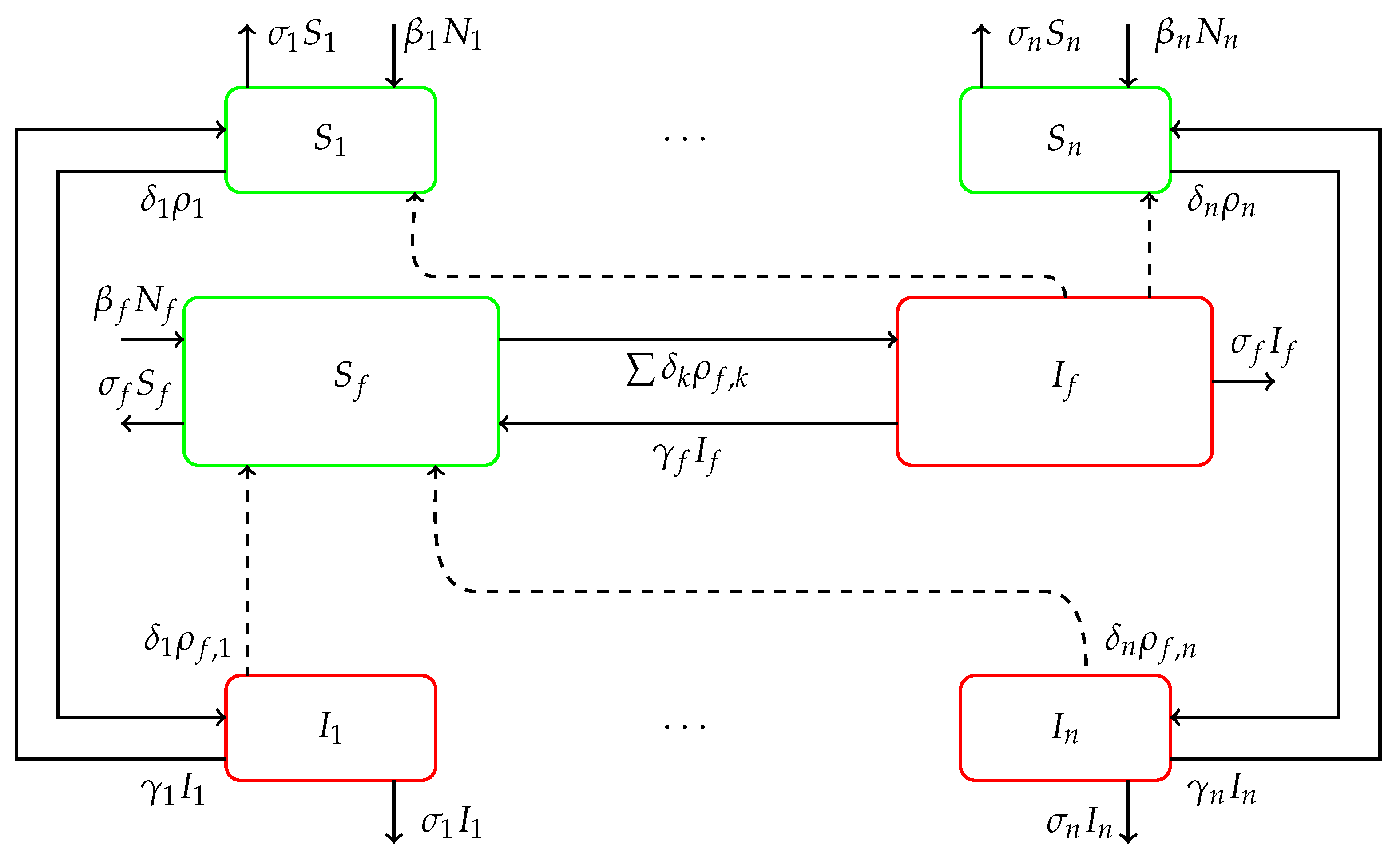
The model presented below builds on the deterministic model in [19]. The CL model in [19] considers $n-1$ animal populations that serve as reservoirs, a human host population, and a single sand flies vector population. The model consists of $n+1$ susceptible classes and $n+1$ infectious classes. In this work, we update all $2(n+1)$ classes of susceptible and infectious populations with time delays that account for the incubation period of the parasite within each population of reservoirs, hosts, and vectors. The schematics of the $2(n+1)$ compartmental SIS model is given in Figure 3. As an example, the susceptible compartment label $S_1$ interacts with infectious sandflies from the compartment $I_f$, resulting in an outflow rate ${\delta }_1{\rho }_1$ into the compartment $I_1$. $S_1$ is also depleted by natural death at rate ${\sigma }_1$. The $S_1$ compartment is populated through a birth rate ${\beta }_1{N}_1$ and recovery rate ${\gamma }_1{I}_1$. The same process is repeated in all $n+1$ susceptible compartments.

The system of equations associated with the schematic diagram that governs the model are:

$$\begin{array}{ll}\hfill \frac{d{S}_k}{dt}& ={\beta }_k{N}_k-{\delta }_k{\rho }_k\frac{S_k\left(t\right)}{N_k}{I}_f(t-{\tau }_k)+{\gamma }_k{I}_k-{\sigma }_k{S}_k,k=1,\dots ,n\hfill \\ \hfill \frac{d{I}_k}{dt}& ={\delta }_k{\rho }_k\frac{S_k\left(t\right)}{N_k}{I}_f(t-{\tau }_k)-{\gamma }_k{I}_k-{\sigma }_k{I}_k,k=1,\dots ,n\hfill \\ \hfill \frac{d{S}_f}{dt}& ={\beta }_f{N}_f-{\displaystyle \sum _{k=1}^n}{\delta }_k{\rho }_{f,k}\frac{I_k(t-{\tau }^{*})}{N_k}{S}_f\left(t\right)+{\gamma }_f{I}_f-{\sigma }_f{S}_f\hfill \\ \hfill \frac{d{I}_f}{dt}& ={\displaystyle \sum _{k=1}^n}{\delta }_k{\rho }_{f,k}\frac{I_k(t-{\tau }^{*})}{N_k}{S}_f\left(t\right)-{\gamma }_f{I}_f-{\sigma }_f{I}_f.\hfill \end{array}$$

(1)

All parameters in the above system of equations are positive and their descriptions are stated in

Table 1. Definition of the parameters of the model.

Parameter	Definition
$S_k$	susceptible human/animal population for $k=1,\dots ,n$
$I_k$	infectious human/animal population for $k=1,\dots ,n$
$N_k$	total human/animal population for $k=1,\dots ,n$
$S_f$	susceptible sandfly population
$I_f$	infectious sandfly population
$N_f$	total sandfly population
${\beta }_k$	birth rate for human/animal for $k=1,\dots ,n$
${\beta }_f$	sandfly reproduction rate
${\sigma }_k$	natural death rate for human/animal for $k=1,\dots ,n$
${\sigma }_f$	sandfly death rate
${\gamma }_k$	recovery rate for human/animal for $k=1,\dots ,n$
${\gamma }_f$	sandfly recovery rate
${\delta }_k$	average biting rate of human/animal by sandflies for $k=1,\dots ,n$
${\rho }_k$	transmission rate from human/animal to sandfly for $k=1,\dots ,n$
${\rho }_{f,k}$	transmission rate from sandfly to human/animal for $k=1,\dots ,n$
${\tau }_k$	incubation period in human/animal population for $k=1,\dots ,n$
${\tau }^{*}$	incubation period in sandfly population

. All susceptible classes are depleted to populate the infectious classes, and are being replenished at some constant birth ($\beta$’s) and recovery ($\gamma$’s) rates. All population groups decay naturally at some constant rate (given by the $\sigma$’s).

We define the initial conditions of the system (1) as

$$\begin{array}{ccc}\hfill S_k\left(0\right)=S_{k0}>0,& I_k\left(t\right)={\varphi }_k\left(t\right)>0,\hfill & \hfill \mathrm{for}k=1,\dots ,n\\ \hfill S_f\left(0\right)=S_{f0}>0,& I_f\left(t\right)=\phi \left(t\right)>0,\hfill \\ \hfill t\in [-\overline{\tau },0],& \overline{\tau }=max\{{\tau }_1,\dots ,{\tau }_n,{\tau }^{*}\},\hfill \end{array}$$

(2)

where ${\varphi }_k\left(t\right)$ for $k=1,\dots ,n$ and $\phi \left(t\right)$ are continuous functions.

Remark 1.

We note here that assumptions such as cutaneous leishmaniasis not leading to any deaths, and equal birth/death rates have been made in the model (1). In this case, the different total populations, $N_1,\dots ,N_n$, and $N_f$ are constant, so that $N_k=S_k\left(t\right)+I_k\left(t\right)$ for $k=1,\dots ,n$, and $N_f=S_f\left(t\right)+I_f\left(t\right)$. (As a consequence it is clear from (1) that $S_k^{\prime }\left(t\right)+I_k^{\prime }\left(t\right)=0$ for $k=1,\dots ,n$, and $S_f^{\prime }\left(t\right)+I_f^{\prime }\left(t\right)=0$).

The following result shows that the model (1) with the initial conditions (2) is well-posed.

Theorem 1.

All solutions of the model (1) with initial conditions (2) are positive and bounded.

Proof. 

Let $t^{*}$ be the smallest positive time value where one of the dependent variables in question turns negative, i.e., $Z\left(t^{*}\right)=0$ and $dZ/dt\left(t^{*}\right)\le 0$ where Z is one of the functions $S_1,\dots ,S_n,I_1,\dots ,I_n,S_f,I_f$. Now this Z can not be any of the $S_k$ functions, because $d{S}_k/dt\left(t^{*}\right)>0$ when $S_k\left(t^{*}\right)=0$ and $t^{*}$ was the smallest positive time value where any of these functions turn negative, i.e., $I_k\left(t^{*}\right)\ge 0$. Similarly, Z can not be any of the $I_k$ functions because $d{I}_k/dt\left(t^{*}\right)>0$ as $S_k\left(t^{*}\right)>0$ and $I_f(t^{*}-{\tau }_k)>0$ because of the minimality of $t^{*}$. Analogous arguments prove that Z can not be $S_f$ or $I_f$ either, thus the statement is verified.

The boundedness of the solutions follow from the fact that the different populations are constant populations with $N_k=S_k\left(t\right)+I_k\left(t\right)$ for $k=1,\dots ,n$ and $N_f=S_f\left(t\right)+I_f\left(t\right)$. □

Remark 2.

Theorem 1 shows that the system (1) with initial conditions (2) is positively invariant on the region defined by

$$\Omega =\{0\le S_f,0\le I_f,0\le S_f+I_f=N_f,0\le S_k,0\le I_k,0\le S_k+I_k=N_k,k=1,\dots ,n\}.$$

Further, by the fundamental theorem of functional differential equations [21], the model admits a unique solution.

3. Analysis of the Model

In this section we derive a threshold value of the model and used it to establish the existence of a positive nonzero equilibrium.

In the analysis that follows, we reduced the $2(n+1)$ system Equations (1) to a smaller system of $n+1$ equations by focusing only on the equations for the infectious populations. We achieve this by eliminating the equations for the susceptible populations using the conservation equations $N_k=S_k\left(t\right)+I_k\left(t\right)$ for $k=1,\dots ,n$ and $N_f=S_f\left(t\right)+I_f\left(t\right)$. Note that we have assumed that ${\beta }_k={\sigma }_k$ for $k=1,\dots ,n$ and ${\beta }_f={\sigma }_f$. The infective equations of the model are now:

$$\begin{array}{cc}\hfill \frac{d{I}_k}{dt}& ={\delta }_k{\rho }_k\frac{(N_k-I_k)}{N_k}{I}_f(t-{\tau }_k)-{\gamma }_k{I}_k-{\sigma }_k{I}_k,k=1,\dots ,n\hfill \\ \hfill \frac{d{I}_f}{dt}& ={\displaystyle \sum _{k=1}^n}{\delta }_k{\rho }_{f,k}\frac{I_k(t-{\tau }^{*})}{N_k}(N_f-I_f)-{\gamma }_f{I}_f-{\sigma }_f{I}_f.\hfill \end{array}$$

We normalize the above equations by defining the dimensionless variables $y=I_f/N_f$ and $x_k=I_k/N_k$ for $k=1,\dots ,n$. The infective equations now become

$$\begin{array}{cc}\hfill \frac{d{x}_k}{dt}& =c_k[{\alpha }_k(1-x_k)y(t-{\tau }_k)-x_k]\hfill \\ \hfill \frac{dy}{dt}& =c_0[(1-y){\displaystyle \sum _{k=1}^n}{\lambda }_k{x}_k(t-{\tau }^{*})-y],\hfill \end{array}$$

(3)

where $y\ge 0$, $x_k\ge 0$ for $k=1,\dots ,n$, $c_0={\sigma }_f+{\gamma }_f$ and $c_k={\sigma }_k+{\gamma }_k$ for $k=1,\dots ,n$ and where

$${\alpha }_k=\frac{{\delta }_k{\rho }_k{N}_f}{({\sigma }_k+{\gamma }_k)N_k},{\lambda }_k=\frac{{\delta }_k{\rho }_{f,k}}{({\sigma }_f+{\gamma }_f)},\mathrm{for}k=1,\dots ,n.$$

From this point forward, for the purpose of simplicity, we assume that ${\tau }_1={\tau }_2=\dots ={\tau }_n=\tau$. It is clear that the normalization leading to the system of the Equations (3) constraints the solution space to the positive unit box $\mathbf{B}=\left\{(x_1,\dots ,x_n,y)\right|0\le x_1,\dots ,x_n\le 1;0\le y\le 1\}$. The following result, which is a consequence of Theorem 1, establishes that the solution domain given by the unit box $\mathbf{B}$ is positively invariant.

Lemma 1.

All solutions of the system (3) that start in the region $\mathbf{B}$ remain in $\mathbf{B}$ for all $t\ge 0$ with the exception of the equilibrium solution at the origin.

The proof of this result follows from Theorem 1.

Next we derive a threshold value of the model (3). It is a useful metric that helps determine whether or not an infectious disease can spread through a population. If the infection is to spread so that we have an outbreak, then we need $\frac{d{x}_k}{dt}>0$ for $k=1,\dots ,n$ and $\frac{dy}{dt}>0$ at $t=0$. Thus we need from (3) that,

$$\begin{array}{ccc}\hfill {\alpha }_k(1-x_k)y(t-\tau )-x_k& >& 0,\mathrm{for}k=1,\dots ,n\hfill \\ \hfill (1-y){\displaystyle \sum _{k=1}^n}{\lambda }_k{x}_k(t-{\tau }^{*})-y& >& 0.\hfill \end{array}$$

The first inequality yields

$${\alpha }_k(1-x_k)y(t-\tau )>x_k,$$

(4)

for $k=1,\dots ,n$, and the second inequality gives

$$(1-y){\displaystyle \sum _{k=1}^n}{\lambda }_k{x}_k(t-{\tau }^{*})>y.$$

(5)

Multiplying both sides of (4) by ${\lambda }_k$ we get

$${\alpha }_k{\lambda }_k(1-x_k)y(t-\tau )>{\lambda }_k{x}_k,$$

for $k=1,\dots ,n$, which upon summing leads to

$${\displaystyle \sum _{k=1}^n}{\alpha }_k{\lambda }_k(1-x_k)y(t-\tau )>{\displaystyle \sum _{k=1}^n}{\lambda }_k{x}_k.$$

(6)

By observing that $1-x_k\le 1$ and $1-y\le 1$, the inequalities in (5) and (6), respectively, become

$${\displaystyle \sum _{k=1}^n}{\lambda }_k{x}_k(t-{\tau }^{*})>y,$$

(7)

and

$${\displaystyle \sum _{k=1}^n}{\alpha }_k{\lambda }_{k}y(t-\tau )>{\displaystyle \sum _{k=1}^n}{\lambda }_k{x}_k.$$

(8)

From (7) and (8) we get that

$${\displaystyle \sum _{k=1}^n}{\alpha }_k{\lambda }_{k}y(t-\tau )>y.$$

Noting again that $y(t-\tau )\le y\left(t\right)$ at the start of the infection, the above inequality becomes

$${\displaystyle \sum _{k=1}^n}{\alpha }_k{\lambda }_k>1.$$

The quantity on the left hand side gives a threshold value of the system (3), and is denoted by $R_0$. Thus, we have

$$R_0={\displaystyle \sum _{k=1}^n}{\alpha }_k{\lambda }_k.$$

Remark 3.

We remark here that the threshold value $R_0$ computed above is equivalent to the basic reproduction number obtained in [19]. The basic reproduction number is the average number of secondary cases caused by introducing an infectious individual in a completely susceptible population. Based on the above computation of the threshold value, we see that each animal/human population $x_k$, contributes ${\alpha }_k{\lambda }_k$ infections towards $R_0$.

Further we note that for each population $x_k$, ${\alpha }_k$ is given as the product of the average time spent in an infectious state $1/({\sigma }_k+{\gamma }_k)$, the sandflies average biting rate ${\delta }_k$, the transmission rate from human/animal to sandflies ${\rho }_k$, and the ratio of total sandflies to human/animal population $N_f/N_k$. Similarly, ${\lambda }_k$ is given as the product of the average time spent by sandflies in an infectious state $1/({\sigma }_f+{\gamma }_f)$, their average biting rate ${\delta }_k$, and the transmission rate from sandflies to human/animal ${\rho }_{f,k}$.

We now turn our attention to computing the equilibriums of the system (3). At the equilibrium points, $({\overline{x}}_1,\dots ,{\overline{x}}_n,\overline{y})$, we have that ${\dot{x}}_k=0$, $(k=1,\dots ,n)$ and $\dot{y}=0$, leading to the equations

$${\overline{x}}_k=\frac{{\alpha }_k\overline{y}}{1+{\alpha }_k\overline{y}},(k=1,\dots ,n)\mathrm{and}{\displaystyle \sum _{k=1}^n}{\lambda }_k{\overline{x}}_k=\frac{\overline{y}}{1-\overline{y}}.$$

Eliminating ${\overline{x}}_k$ from the above equations yields the following equation:

$${\displaystyle \sum _{k=1}^n}\frac{{\alpha }_k{\lambda }_k\overline{y}}{1+{\alpha }_k\overline{y}}-\frac{\overline{y}}{1-\overline{y}}=0.$$

(9)

The Equation (9) governs the equilibriums of the system and an immediate observation is that $\overline{y}=0$ and consequently $({\overline{x}}_1,\dots ,{\overline{x}}_n,\overline{y})=(0,\dots ,0,0)$ is an equilibrium point. We call $(0,\dots ,0,0)$ the disease-free equilibrium (DFE) of the model (3). Further, using the Equation (9), the following result establishes the existence of a unique positive equilibrium other than the DFE, which we refer to as the endemic equilibrium.

Theorem 2

([19]). System (3) has a unique equilibrium solution with positive coordinates if the threshold value $R_0={\sum }_{k=1}^n{\alpha }_k{\lambda }_k>1$. If $R_0\le 1$, the system has no equilibria with positive coordinates. The origin is an equilibrium in all cases.

The proof of this result is given in Theorem 3.1 in Agyingi et al. [19].

We remark here that the equations defining the equilibrium points are identical to the equations for the ordinary differential equation model in [19], thus the result describing the equilibriums is also identical. We will investigate the stability of the DFE and the endemic equilibrium in Section 4 and Section 5 respectively.

4. Analysis of the Disease-Free Equilibrium

In this section we study the long term behavior of the disease-free equilibrium of the proposed model. We start by computing the characteristic equation of the delay system (3) which is given as

$$\det ({\mathbf{J}}_0+e^{-s\tau }{\mathbf{J}}_{\tau }+e^{-s{\tau }^{*}}{\mathbf{J}}_{{\tau }^{*}}-s\mathbf{I})=0,$$

(10)

where $\mathbf{I}$ is the $(n+1)\times (n+1)$ identity matrix and where the Jacobian matrices ${\mathbf{J}}_0$, ${\mathbf{J}}_{\tau }$, and ${\mathbf{J}}_{{\tau }^{*}}$ are defined respectively as

$${\mathbf{J}}_0=\left[\begin{array}{ccccc}-c_1{\alpha }_{1}y-c_1& 0& 0& \cdots & 0\\ 0& -c_2{\alpha }_{2}y-c_2& 0& \cdots & 0\\ ⋮& \ddots & \ddots & \ddots & ⋮\\ ⋮& 0& -c_n{\alpha }_{n}y-c_n& 0\\ 0& \cdots & \cdots & 0& -c_0{\displaystyle \sum _{k=1}^n}{\lambda }_k{x}_k-c_0\end{array}\right],$$

$${\mathbf{J}}_{\tau }=\left[\begin{array}{ccccc}0& 0& \cdots & 0& c_1{\alpha }_1(1-x_1)\\ 0& 0& \cdots & 0& c_2{\alpha }_2(1-x_2)\\ ⋮& ⋮& ⋮& ⋮\\ 0& 0& \cdots & 0& c_n{\alpha }_n(1-x_n)\\ 0& 0& \cdots & 0& 0\end{array}\right]\mathrm{and}$$

$${\mathbf{J}}_{{\tau }^{*}}=\left[\begin{array}{ccccc}0& 0& \cdots & 0& 0\\ 0& 0& \cdots & 0& 0\\ ⋮& ⋮& ⋮& ⋮\\ 0& 0& \cdots & 0& 0\\ c_0{\lambda }_1(1-y)& c_0{\lambda }_2(1-y)& \cdots & c_0{\lambda }_n(1-y)& 0\end{array}\right].$$

Bearing in mind that the origin is the DFE of the system, the characteristic equation evaluated at the DFE yields

$$\det \left[\begin{array}{ccccc}-c_1-s& 0& \cdots & 0& e^{-s\tau }{c}_1{\alpha }_1\\ 0& -c_2-s& \ddots & ⋮& e^{-s\tau }{c}_2{\alpha }_2\\ ⋮& \ddots & \ddots & 0& ⋮\\ 0& \cdots & 0& -c_n-s& e^{-s\tau }{c}_n{\alpha }_n\\ e^{-s{\tau }^{*}}{c}_0{\lambda }_1& e^{-s{\tau }^{*}}{c}_0{\lambda }_2& \cdots & e^{-s{\tau }^{*}}{c}_0{\lambda }_n& -c_0-s\end{array}\right]=0,$$

and on evaluating the above determinant, the characteristic equation at the disease-free equilibrium becomes

$$\begin{array}{c}\hfill {(-1)}^{n+1}{\displaystyle \prod _{j=0}^n}(c_j+s)+{(-1)}^n{e}^{-s(\tau +{\tau }^{*})}{c}_0{\displaystyle \sum _{k=1}^n}{\displaystyle \prod _{j=1;j\ne k}^n}(c_j+s)c_k{\alpha }_k{\lambda }_k=0.\end{array}$$

(11)

Theorem 3.

The disease-free equilibrium of the system (3) is unstable if $R_0>1$ and stable if $R_0<1$.

Proof. 

We begin by showing that the disease-free equilibrium is unstable if $R_0>1$. Denoting the function on the left side of (11) by $f\left(s\right)$, that is,

$$\begin{array}{c}\hfill f\left(s\right)={(-1)}^{n+1}{\displaystyle \prod _{j=0}^n}(c_j+s)+{(-1)}^n{e}^{-s(\tau +{\tau }^{*})}{c}_0{\displaystyle \sum _{k=1}^n}{\displaystyle \prod _{j=1;j\ne k}^n}(c_j+s)c_k{\alpha }_k{\lambda }_k,\end{array}$$

(12)

when $s=0$, we get

$$f\left(0\right)={(-1)}^{n+1}{\displaystyle \prod _{j=0}^n}{c}_j+{(-1)}^n{\displaystyle \prod _{j=0}^n}{c}_j{\displaystyle \sum _{k=1}^n}{\alpha }_k{\lambda }_k.$$

Observing that ${\sum }_{k=1}^n{\alpha }_k{\lambda }_k=R_0$, the preceding equation becomes

$$\begin{array}{c}\hfill f\left(0\right)={(-1)}^n{\displaystyle \prod _{j=0}^n}{c}_j[R_0-1].\end{array}$$

(13)

We see from (12) that if n is odd, then $f\left(s\right)\to \infty$ as $s\to \infty$, and if $R_0>1$ in (13) then $f\left(0\right)<0$. Similarly, if n is even, then $f\left(s\right)\to -\infty$ as $s\to \infty$, and $f\left(0\right)>0$ as long as $R_0>1$. Thus there exists a positive real root of $f\left(s\right)$, establishing the instability of the disease-free equilibrium.

Next we show that the disease-free equilibrium is stable if $R_0<1$. Re-writing Equation (11) and dividing both sides by ${(-1)}^{n+1}$, we obtain

$$\begin{array}{c}\hfill {\displaystyle \prod _{j=0}^n}(c_j+s)=e^{-s(\tau +{\tau }^{*})}{c}_0{\displaystyle \sum _{k=1}^n}{\displaystyle \prod _{j=1;j\ne k}^n}(c_j+s)c_k{\alpha }_k{\lambda }_k,\end{array}$$

which is equivalent to

$$\begin{array}{c}\hfill c_0+s=e^{-s(\tau +{\tau }^{*})}{c}_0\left(\frac{c_1{\alpha }_1{\lambda }_1}{c_1+s}+\frac{c_2{\alpha }_2{\lambda }_2}{c_2+s}+\cdots +\frac{c_n{\alpha }_n{\lambda }_n}{c_n+s}\right).\end{array}$$

(14)

Suppose that there is a $s\ge 0$ which satisfies the above equation, then we have that,

$$\begin{array}{cc}\hfill c_0+s& =e^{-s(\tau +{\tau }^{*})}{c}_0\left(\frac{c_1{\alpha }_1{\lambda }_1}{c_1+s}+\frac{c_2{\alpha }_2{\lambda }_2}{c_2+s}+\cdots +\frac{c_n{\alpha }_n{\lambda }_n}{c_n+s}\right)\hfill \\ & <e^{-s(\tau +{\tau }^{*})}{c}_0\left(\frac{c_1{\alpha }_1{\lambda }_1}{c_1}+\frac{c_2{\alpha }_2{\lambda }_2}{c_2}+\cdots +\frac{c_n{\alpha }_n{\lambda }_n}{c_n}\right)\hfill \\ & =e^{-s(\tau +{\tau }^{*})}{c}_0{\displaystyle \sum _{k=1}^n}{\alpha }_k{\lambda }_k\hfill \\ & =e^{-s(\tau +{\tau }^{*})}{c}_0{R}_0.\hfill \end{array}$$

We get from the above computation that

$$\begin{array}{c}\hfill s<c_0\left(\frac{R_0}{e^{s(\tau +{\tau }^{*})}}-1\right).\end{array}$$

(15)

If $s\ge 0$ and $R_0<1$, then the righthand side of the inequality (15) is negative which is a contradiction. Therefore all real eigenvalues are negative when $R_0<1$.

Further, we investigate whether there are complex eigenvalues with positive real parts. Suppose that $s=\nu +i\omega$, where $\nu ,\omega >0$, then from Equation (14) we get

$$\begin{array}{c}\hfill c_0+\nu +i\omega =e^{-(\nu +i\omega )(\tau +{\tau }^{*})}{c}_0\left(\frac{c_1{\alpha }_1{\lambda }_1}{c_1+\nu +i\omega }+\frac{c_2{\alpha }_2{\lambda }_2}{c_2+\nu +i\omega }+\cdots +\frac{c_n{\alpha }_n{\lambda }_n}{c_n+\nu +i\omega }\right).\end{array}$$

Re-writing the above equation we get

$$\begin{array}{cc}\hfill 1+\frac{\nu }{c_0}+i\frac{\omega }{c_0}& =e^{-\nu (\tau +{\tau }^{*})}[cos\left(\omega (\tau +{\tau }^{*})\right)-isin\left(\omega (\tau +{\tau }^{*})\right)]\hfill \\ & \times \left(\frac{c_1{\alpha }_1{\lambda }_1}{{(c_1+\nu )}^2+{\omega }^2}(c_1+\nu -i\omega )+\cdots +\frac{c_n{\alpha }_n{\lambda }_n}{{(c_n+\nu )}^2+{\omega }^2}(c_n+\nu -i\omega )\right).\hfill \end{array}$$

Equating the real and imaginary parts of the above equation we respectively obtain

$$\begin{array}{cc}\hfill 1+\frac{\nu }{c_0}& =cos\left(\omega (\tau +{\tau }^{*})\right)\left(\frac{c_1{\alpha }_1{\lambda }_1(c_1+\nu )}{{(c_1+\nu )}^2+{\omega }^2}+\cdots +\frac{c_n{\alpha }_n{\lambda }_n(c_n+\nu )}{{(c_n+\nu )}^2+{\omega }^2}\right)e^{-\nu (\tau +{\tau }^{*})}\hfill \\ & -\omega sin\left(\omega (\tau +{\tau }^{*})\right)\left(\frac{c_1{\alpha }_1{\lambda }_1}{{(c_1+\nu )}^2+{\omega }^2}+\cdots +\frac{c_n{\alpha }_n{\lambda }_n}{{(c_n+\nu )}^2+{\omega }^2}\right)e^{-\nu (\tau +{\tau }^{*})}.\hfill \end{array}$$

(16)

and

$$\begin{array}{cc}\hfill \frac{\omega }{c_0}& =-\omega cos\left(\omega (\tau +{\tau }^{*})\right)\left(\frac{c_1{\alpha }_1{\lambda }_1}{{(c_1+\nu )}^2+{\omega }^2}+\cdots +\frac{c_n{\alpha }_n{\lambda }_n}{{(c_n+\nu )}^2+{\omega }^2}\right)e^{-\nu (\tau +{\tau }^{*})}\hfill \\ & -sin\left(\omega (\tau +{\tau }^{*})\right)\left(\frac{c_1{\alpha }_1{\lambda }_1(c_1+\nu )}{{(c_1+\nu )}^2+{\omega }^2}+\cdots +\frac{c_n{\alpha }_n{\lambda }_n(c_n+\nu )}{{(c_n+\nu )}^2+{\omega }^2}\right)e^{-\nu (\tau +{\tau }^{*})}.\hfill \end{array}$$

(17)

Adding the squares of both sides of Equations (16) and (17), we get that

$$\begin{array}{cc}\hfill {\left(1+\frac{\nu }{c_0}\right)}^2+\frac{{\omega }^2}{c_0^2}& =\left[{\left({\displaystyle \sum _{k=1}^n}\frac{c_k{\alpha }_k{\lambda }_k(c_k+\nu )}{{(c_k+\nu )}^2+{\omega }^2}\right)}^2+{\left(\omega {\displaystyle \sum _{k=1}^n}\frac{c_k{\alpha }_k{\lambda }_k}{{(c_k+\nu )}^2+{\omega }^2}\right)}^2\right]e^{-2\nu (\tau +{\tau }^{*})}\hfill \\ & <{\left({\displaystyle \sum _{k=1}^n}\frac{c_k{\alpha }_k{\lambda }_k(c_k+\nu )}{{(c_k+\nu )}^2+{\omega }^2}\right)}^2+{\omega }^2{\left({\displaystyle \sum _{k=1}^n}\frac{c_k{\alpha }_k{\lambda }_k}{{(c_k+\nu )}^2+{\omega }^2}\right)}^2\hfill \\ & <{\left({\displaystyle \sum _{k=1}^n}\frac{c_k{\alpha }_k{\lambda }_k}{(c_k+\nu )}\right)}^2+{\omega }^2{\left({\displaystyle \sum _{k=1}^n}\frac{c_k{\alpha }_k{\lambda }_k}{{(c_k+\nu )}^2}\right)}^2\hfill \\ & <{\left({\displaystyle \sum _{k=1}^n}\frac{c_k{\alpha }_k{\lambda }_k}{c_k}\right)}^2+{\omega }^2{\left({\displaystyle \sum _{k=1}^n}\frac{c_k{\alpha }_k{\lambda }_k}{c_k^2}\right)}^2\hfill \\ & <{\left({\displaystyle \sum _{k=1}^n}{\alpha }_k{\lambda }_k\right)}^2+{\omega }^2{\left({\displaystyle \sum _{k=1}^n}\frac{{\alpha }_k{\lambda }_k}{c_k}\right)}^2<R_0^2+\frac{{\omega }^2}{c_{*}^2}{R}_0^2,\hfill \end{array}$$

where $c_{*}=min\{c_1,c_2,\dots ,c_n\}$. The above inequality yields

$$\begin{array}{c}\hfill {\left(1+\frac{\nu }{c_0}\right)}^2+\frac{{\omega }^2}{c_0^2}<R_0^2\left(1+\frac{{\omega }^2}{c_{*}^2}\right),\end{array}$$

which cannot be satisfied by any positive $\nu$ and $\omega$ values when $R_0<1$, if we impose the sufficient condition that $c_{*}\ge c_0$. Therefore there are no complex eigenvalues with positive real parts. Also observe that if $\nu =0$, there are no imaginary eigenvalues since no $\omega >0$ satisfies the above inequality. We conclude that the disease-free equilibrium is locally asymptotically stable. □

Remark 4.

The condition that $c_{*}\ge c_0$ in the above proof is only a sufficient condition since the disease-free equilibrium does not exhibit any form of instabilities. The disease-free equilibrium remains stable even when $c_{*}\le c_0$ as demonstrated in the next result.

We complete our analysis of the disease-free equilibrium by providing the following global stability result, which is stronger than local stability whenever the threshold value $R_0$ is smaller than 1.

Theorem 4.

The disease-free equilibrium of the system (3) is globally asymptotically stable if $R_0<1$.

Proof. 

We start with the first equation of the system (3), that is, for $k=1,\dots ,n$ we have

$$\frac{d{x}_k}{dt}=c_k[{\alpha }_k(1-x_k)y(t-\tau )-x_k].$$

Recalling from Remark 1 that all solutions are contained within a unit box, we have the differential inequalities

$$\frac{d{x}_k}{dt}\le c_k[{\alpha }_{k}y(t-\tau )-x_k],k=1,\dots ,n,$$

which are the same as

$$\frac{d{x}_k}{dt}+c_k{x}_k\le c_k{\alpha }_{k}y(t-\tau )k=1,\dots ,n.$$

Multiplying both sides of the preceding inequalities by $e^{c_{k}t}$, we obtain that

$$\frac{d{x}_k}{dt}{e}^{c_{k}t}+c_k{x}_k{e}^{c_{k}t}=\frac{d}{dt}\left(x_k\left(t\right)e^{c_{k}t}\right)\le c_k{\alpha }_k{e}^{c_{k}t}y(t-\tau ),k=1,\dots ,n.$$

Integrating the above inequalities on the interval $(0,t)$, we obtain

$$x_k\left(t\right)e^{c_{k}t}-x_k\left(0\right)\le {\int }_0^t{c}_k{\alpha }_k{e}^{c_{k}s}y(s-\tau )ds,k=1,\dots ,n.$$

Rearranging these inequalities, we have that

$$x_k\left(t\right)\le e^{-c_{k}t}{x}_k\left(0\right)+e^{-c_{k}t}{\int }_0^t{c}_k{\alpha }_k{e}^{c_{k}s}y(s-\tau )ds,k=1,\dots ,n.$$

Now this implies that for $k=1,\dots ,n$,

$$x_k\left(t\right)\le e^{-c_{k}t}{x}_k\left(0\right)+e^{-c_{k}t}supy\left(t\right){\int }_0^t{c}_k{\alpha }_k{e}^{c_{k}s}ds=e^{-c_{k}t}{x}_k\left(0\right)+supy\left(t\right)({\alpha }_k-{\alpha }_k{e}^{-c_{k}t}).$$

Thus we get that

$$\underset{t}{lim\; sup}{x}_k\left(t\right)\le {\alpha }_k\underset{t}{lim\; sup}y\left(t\right),k=1,\dots ,n.$$

(18)

In a similar fashion, taking the second equation of the system (3), that is,

$$\frac{dy}{dt}=c_0[(1-y){\displaystyle \sum _{k=1}^n}{\lambda }_k{x}_k(t-{\tau }^{*})-y],$$

andbearing in mind Remark 1, we obtain the differential inequality

$$\frac{dy}{dt}\le c_0[{\displaystyle \sum _{k=1}^n}{\lambda }_k{x}_k(t-{\tau }^{*})-y],$$

which is the same as

$$\frac{dy}{dt}+c_{0}y\le c_0[{\displaystyle \sum _{k=1}^n}{\lambda }_k{x}_k(t-{\tau }^{*})].$$

Again, multiplication by $e^{c_{0}t}$ gives

$$\frac{dy}{dt}{e}^{c_{0}t}+c_{0}y{e}^{c_{0}t}=\frac{d}{dt}\left(y\left(t\right)e^{c_{0}t}\right)\le c_0{e}^{c_{0}t}[{\displaystyle \sum _{k=1}^n}{\lambda }_k{x}_k(t-{\tau }^{*})],$$

andthen integration on the interval $(0,t)$ yields

$$e^{c_{0}t}y\left(t\right)-y\left(0\right)\le {\int }_0^t{c}_0{e}^{c_{0}s}{\lambda }_1{x}_1(s-{\tau }^{*})ds+\cdots +{\int }_0^t{c}_0{e}^{c_{0}s}{\lambda }_n{x}_n(s-{\tau }^{*})ds.$$

We again rewrite this as

$$y\left(t\right)\le e^{-c_{0}t}y\left(0\right)+e^{-c_{0}t}{\int }_0^t{c}_0{e}^{c_{0}s}{\lambda }_1{x}_1(s-{\tau }^{*})ds+\cdots +e^{-c_{0}t}{\int }_0^t{c}_0{e}^{c_{0}s}{\lambda }_n{x}_n(s-{\tau }^{*})ds.$$

Taking the supremums we get

$$supy\left(t\right)\le e^{-c_{0}t}y\left(0\right)+e^{c_{0}t}sup{x}_1\left(t\right){\int }_0^t{c}_0{e}^{c_{0}s}{\lambda }_{1}ds+\cdots +e^{c_{0}t}sup{x}_n\left(t\right){\int }_0^t{c}_0{e}^{c_{0}s}{\lambda }_{n}ds.$$

After integration, we then obtain

$$\underset{t}{lim\; sup}y\left(t\right)\le {\lambda }_1\underset{t}{lim\; sup}{x}_1\left(t\right)+\cdots +{\lambda }_n\underset{t}{lim\; sup}{x}_n\left(t\right).$$

(19)

Combining the inequalities (18) and (19), we get

$$\underset{t}{lim\; sup}y\left(t\right)\le {\alpha }_1{\lambda }_1\underset{t}{lim\; sup}y\left(t\right)+\cdots +{\alpha }_n{\lambda }_n\underset{t}{lim\; sup}y\left(t\right)=\underset{t}{lim\; sup}y\left(t\right){\displaystyle \sum _{k=1}^n}{\alpha }_k{\lambda }_k.$$

The preceding inequality is the same as

$$\underset{t}{lim\; sup}y\left(t\right)\le R_0\underset{t}{lim\; sup}y\left(t\right).$$

Since $R_0<1$, we get that $\underset{t}{lim\; sup}y\left(t\right)=0$; consequently, by (18), $\underset{t}{lim\; sup}{x}_k\left(t\right)=0$ for $k=1,\dots ,n$. This concludes the proof. □

5. Numerical Results and Discussion

In this section, we continue our analysis of the equilibriums by considering the case $n=2$ of the system (3), where the $x_1$ variable represents a proportion of infectious human population, $x_2$ variable represents a proportion of infectious animal population and y is a proportion of infectious sandflies. Here we numerically confirm the theoretical results established in the previous section on the stability of the disease-free equilibrium. Next we investigate the stability of the endemic equilibrium for different parameter values of the model, in particular, the population densities and time delays.

The parameter values used in the analysis are mostly similar to parameter values in related works [17,18,19], or arbitrarily chosen to explore the behavior of the model. The average biting rates of human and animal by sandflies are equal and set at ${\delta }_1={\delta }_2=0.25$per day. The transmission rate from human and animal to sandflies are also equal and set at ${\rho }_1={\rho }_2=0.25$. The transmission rate from sandflies to humans and animals are equal and set at ${\rho }_{f,1}={\rho }_{f,2}=0.25$. The death rate of humans, animals and sandflies respectively are ${\sigma }_1=0.0001$per day, ${\sigma }_2=1/365$per day, and ${\sigma }_f=1/14$per day. Values for the recovery rates of humans, animals and sandflies respectively are ${\gamma }_1=12/365$per day, ${\gamma }_2=5/365$per day and ${\gamma }_f=1/14$ per day.

Because animals are mostly the reservoir of the parasite, the initial conditions for all simulations reported below were set at $x_1\left(0\right)=0$, $x_2\left(0\right)=0.1$ and $y\left(0\right)=0$. We performed multiple simulations in which the initial conditions were perturbed and no changes in the behavior of the equilibrium solutions were observed.

In the simulations that follow, we use two sets of time delays, $\{\tau =28,{\tau }^{*}=14\}$ which is well within the known incubation periods, and extreme values $\{\tau =1000,{\tau }^{*}=1000\}$ which are biologically impossible. The very extreme set of time delays was chosen simply to investigate the nature of the stability of the endemic equilibrium, that is, whether there exist critical delay values at which bifurcations take place.

The calculated threshold value $R_0$ of the system for the stated parameter values is given as $R_0={\alpha }_1{\lambda }_1+{\alpha }_2{\lambda }_2$, or $R_0=0.2985N_f/N_1+0.5988N_f/N_2$. It is therefore evident that the sandflies to human/animal ratios determines whether $R_0<1$ or $R_0>1$. We examine each of these cases below.

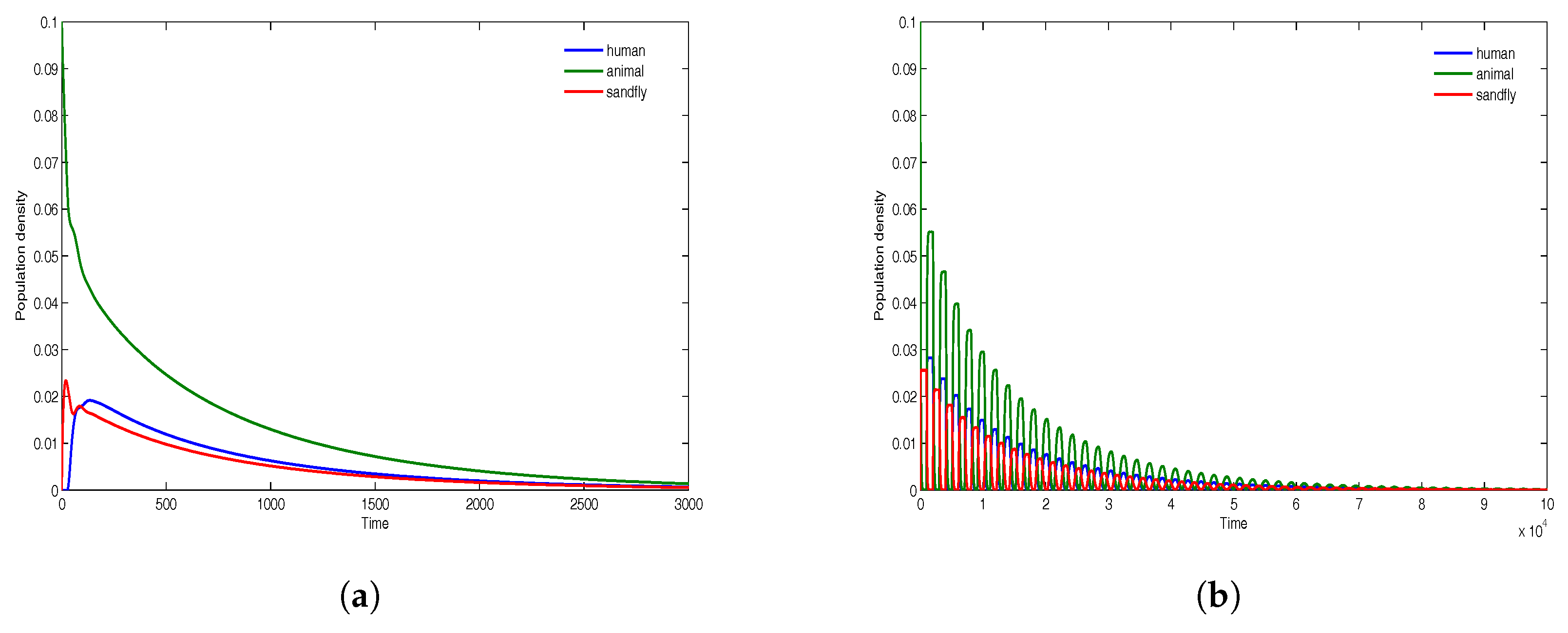
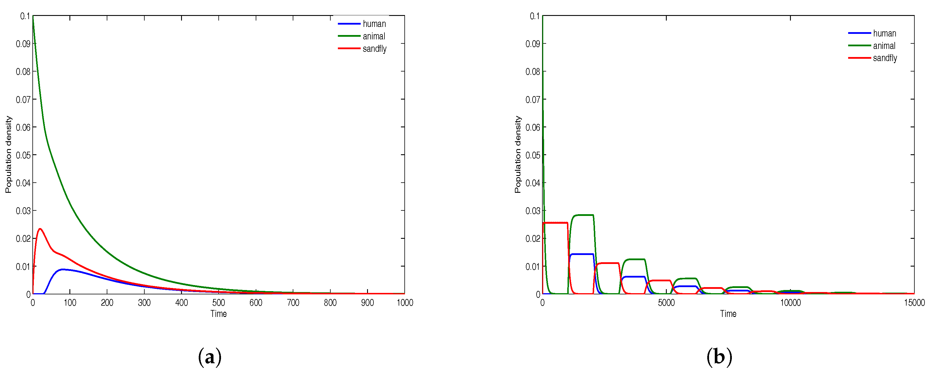
We begin with the case where the ratios $N_f/N_k\le 1$ for $k=1,2$ and where $R_0<1$. The time evolution of all infectious classes is demonstrated in Figure 4, where there are fewer sandflies compare to humans/animals, and in Figure 5, where the densities of sandflies, humans and animals are equal. For population densities $N_1=N_2=5000$ and $N_f=2500$, the results in Figure 4a are for the time delays $\{\tau =28,{\tau }^{*}=14\}$, while the results in Figure 4b are for the time delays $\{\tau ={\tau }^{*}=1000\}$. Similarly, for equal population densities $N_1=N_2=N_f=12,500$, the results in Figure 5a are for the time delays $\{\tau =28,{\tau }^{*}=14\}$, while the results in Figure 5b are for the time delays $\{\tau ={\tau }^{*}=1000\}$. The results in Figure 4 and Figure 5 show that the disease dies out in both cases since $R_0<1$. The presence of very large delays only induces small oscillations whose amplitude decreases with time and all solutions converge to the disease-free equilibrium that is asymptotically stable.

We now turn our attention to the case where for $k=1,2$, the ratios $N_f/N_k>1$ and where $R_0>1$. First we note that it is possible for all $k=1,2$, the ratios $N_f/N_k>1$ to still lead to $R_0<1$. As an example, if $N_f=5200$, and $N_1=N_2=5000$ then we get $R_0=0.9332<1$, leading to the stability of the DFE. Since the endemic equilibrium only exists if $R_0>1$, we focus on those cases where at least one of the ratios $N_f/N_k\gg 1$ for $k=1,2$ and that $R_0>1$.

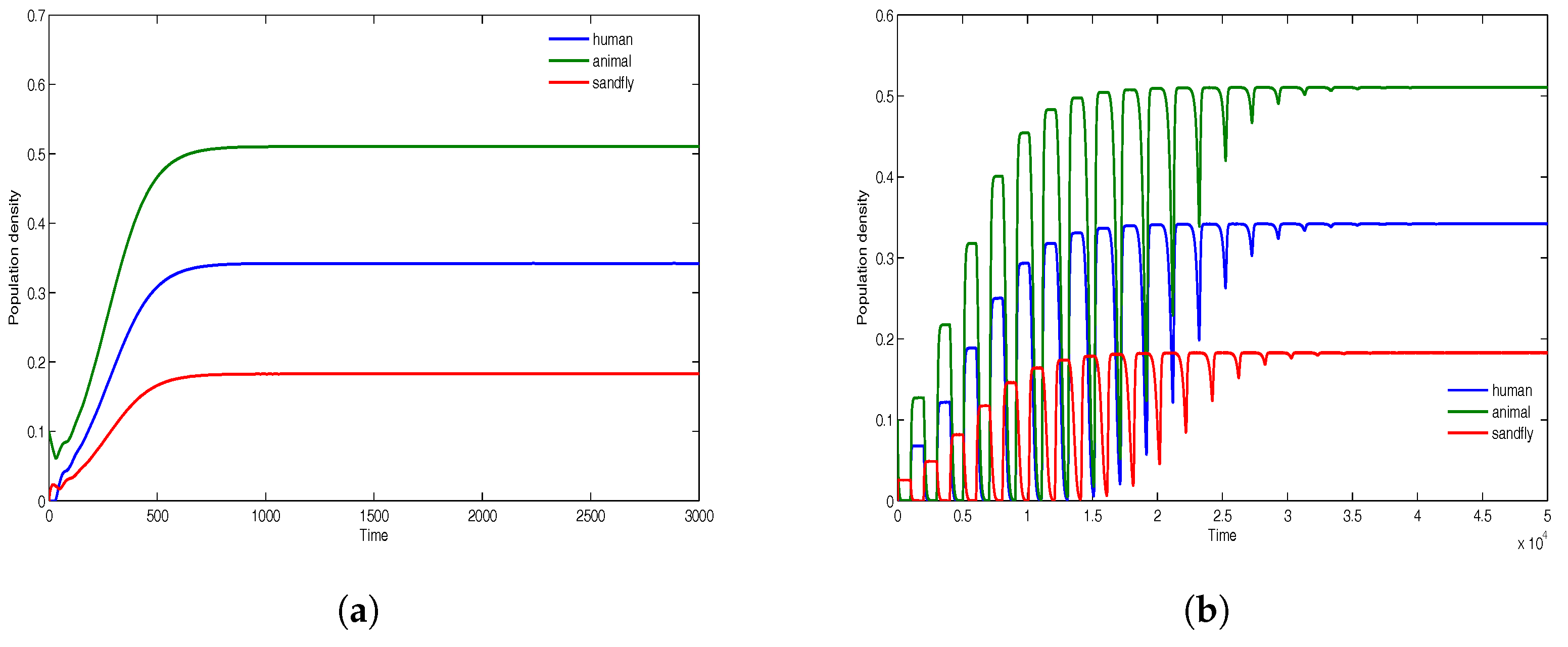
The simulations in Figure 6 give the solution profiles of the model for population densities $N_1=N_2=5000$ and $N_f=12,500$. The computations in Figure 6a are for the time delays $\{\tau =28,{\tau }^{*}=14\}$, while those in Figure 6b are for the time delays $\{\tau ={\tau }^{*}=1000\}$. The results indicate the global stability of the endemic equilibrium. Given very large time delays as illustrated in Figure 6b, the endemic equilibrium at the onset induces some form of instability that grows with time and on attaining maximum amplitude begins to fissile out, and then eventually becomes stable. Although the human and animal population densities are equal, the results in Figure 6 show that the disease is more prevalent in the animal reservoir. This can be attributed to the initial conditions.

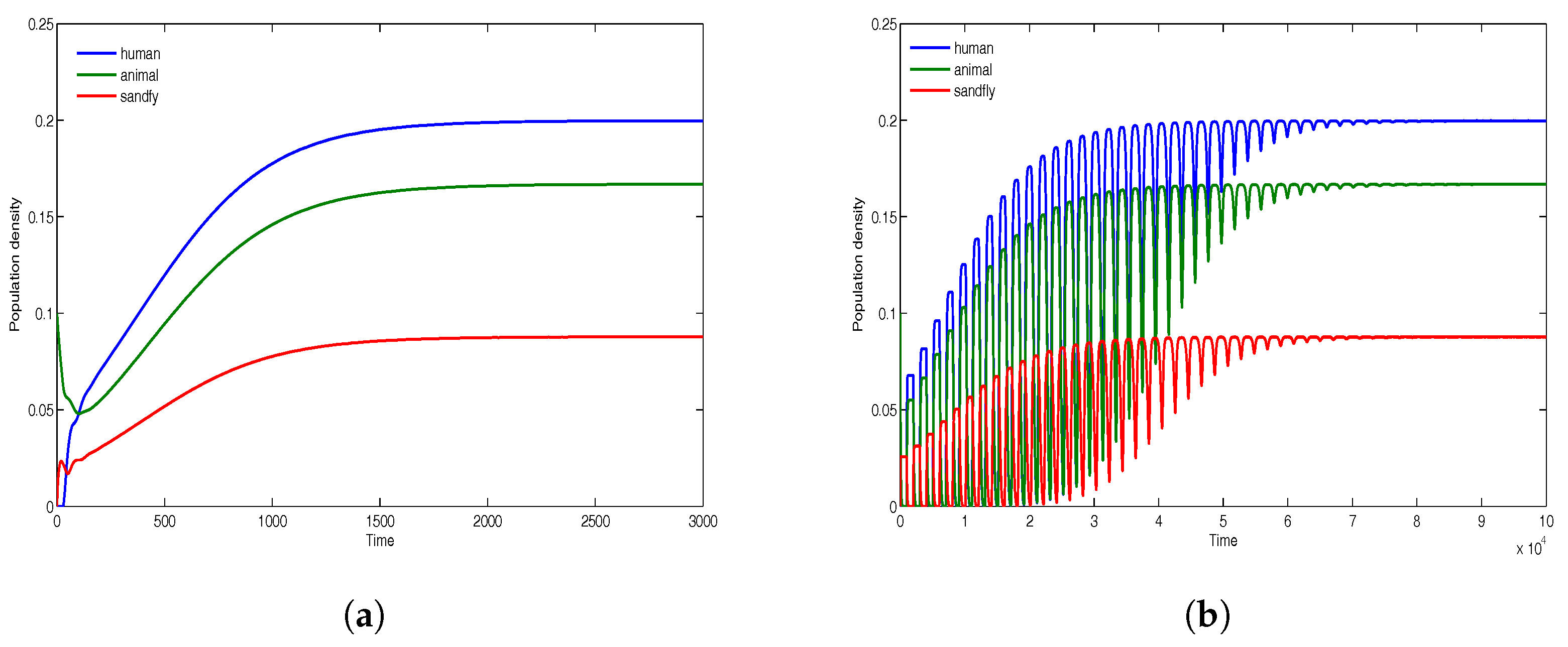
The next results given in Figure 7 are for population densities $N_1=5000$, $N_2=12,500$ and $N_f=12,500$. As in previous computations, Figure 7a is for time delays $\{\tau =28,{\tau }^{*}=14\}$ and Figure 7b is for time delays $\{\tau ={\tau }^{*}=1000\}$. The simulations in Figure 7 also indicate the global stability of the endemic equilibrium. Exceedingly large time delays that initially rattle the solutions (see Figure 7b), do not render the endemic equilibrium unstable with time. We also observe here that when the animal (reservoir) population is significantly higher than that of human, then the model predicts higher disease prevalence among humans.

Finally, we consider the case with population densities $N_1=12,500$, $N_2=2500$ and $N_f=12,500$. Note that in this case, the reservoir density is significantly lower than that of human. The simulations given in Figure 8 indicate a very high level of disease prevalence in the reservoir population and the least disease prevalence among humans. This is unlike in all other cases indicated above where the least prevalence has always been among sandflies.

6. Conclusions

In this paper we have presented a model with time delays for the transmission dynamics of cutaneous leishmaniasis, an infectious disease whose prevalence is on the increase. Although mostly located in tropical regions, global warming may provide suitable conditions for its vector to migrate to subtropical regions and spread the disease. The life cycle of the parasite begins in animals which are usually the reservoirs and manifest as some form of the disease in humans via sandflies transmission.

Mathematical models for leishmaniasis pale in comparison to other infectious diseases and as noted before, only a handful of such models account for the incubation period of the parasite within reservoirs, vectors and humans. The novelty of the model constructed here is that time delays serving as the incubation period have been incorporated into all population groups, which has often been avoided or neglected in past works. Starting with an existing deterministic SIS model, delays were inserted into the $2(n+1)$ dimensional system of equations. Because all populations involved were assumed to be constant, the dimension of the model studied was reduced to a system of only $n+1$ infective equations by eliminating the susceptible terms.

A threshold value $R_0$ of the model was computed as a sum of the products of the infected sandflies and the resulting human/animal infections for each human/animal population group. We used $R_0$ to analyze equilibriums of the model. The disease-free equilibrium of the model is both locally and globally stable when $R_0<1$. A numerical study of the positive endemic equilibrium for the case $n=2$ which only exist when $R_0>1$, shows that it is globally asymptotically stable even when very extreme time delay values are employed.

From the model simulations we observe that as long as the sandflies population is kept lower or near the level of the human and animal populations, the disease will die out. We also learn that if the sandflies population is substantially higher than that of humans and/or animals, the disease will persist in all populations. In the situation where the disease is persistent, the model predicts the following: (i) the prevalence is higher in animals for equal human and animal populations; (ii) the prevalence is higher in humans when the human population is smaller than that of animals; and (iii) the prevalence is least in humans when the animal population is smaller than the human population.

The main limitation of the model presented in this work is the assumption that all infected hosts will survive the incubation period. A possible way of addressing that is the inclusion of an exponential decay term that represents the average proportion of infected individuals which survive the incubation period. The threshold value $R_0$ then will depend on the incubation periods as well.