Augmented Lagrangian Approach to the Newsvendor Model with Component Commonality


Abstract
1. Introduction
2. Literature Review
2.1. Component Commonality
2.2. Primal-Dual Proximal Methods
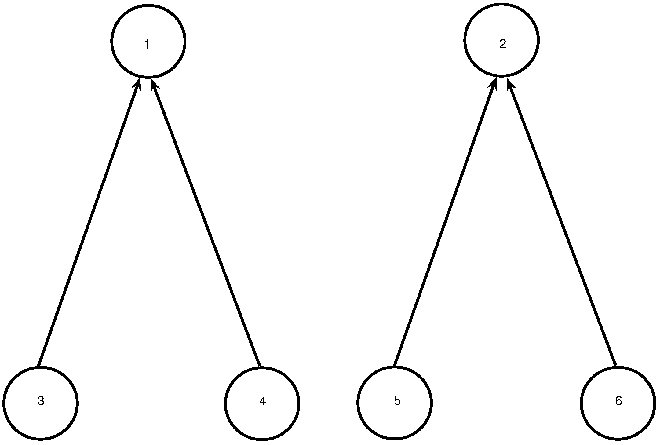
3. Model N
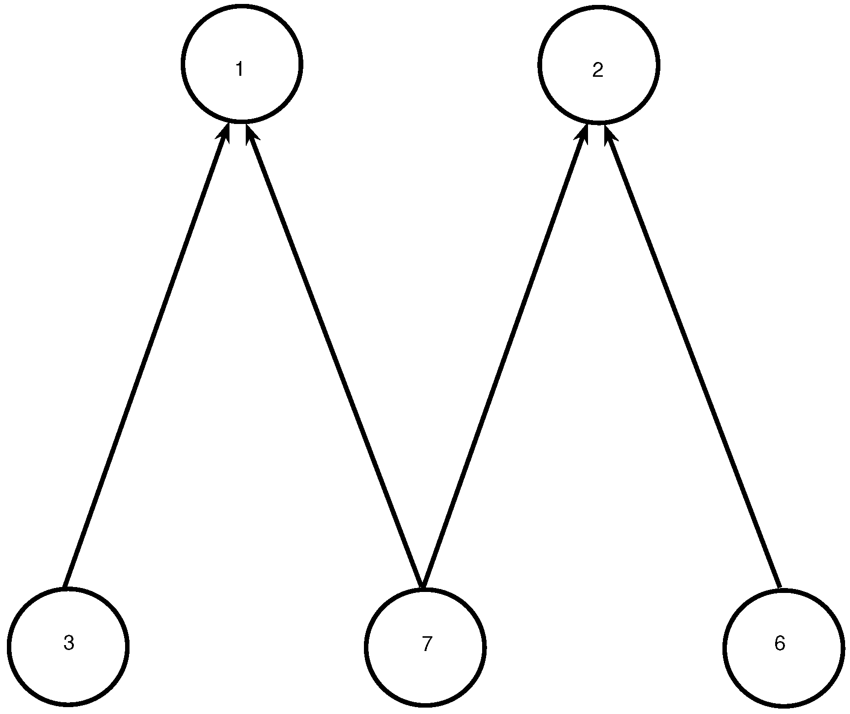
4. Model C
5. Numerical Approach to Model C
| Algorithm 1: Implementation of the proximal multipliers method. |
|
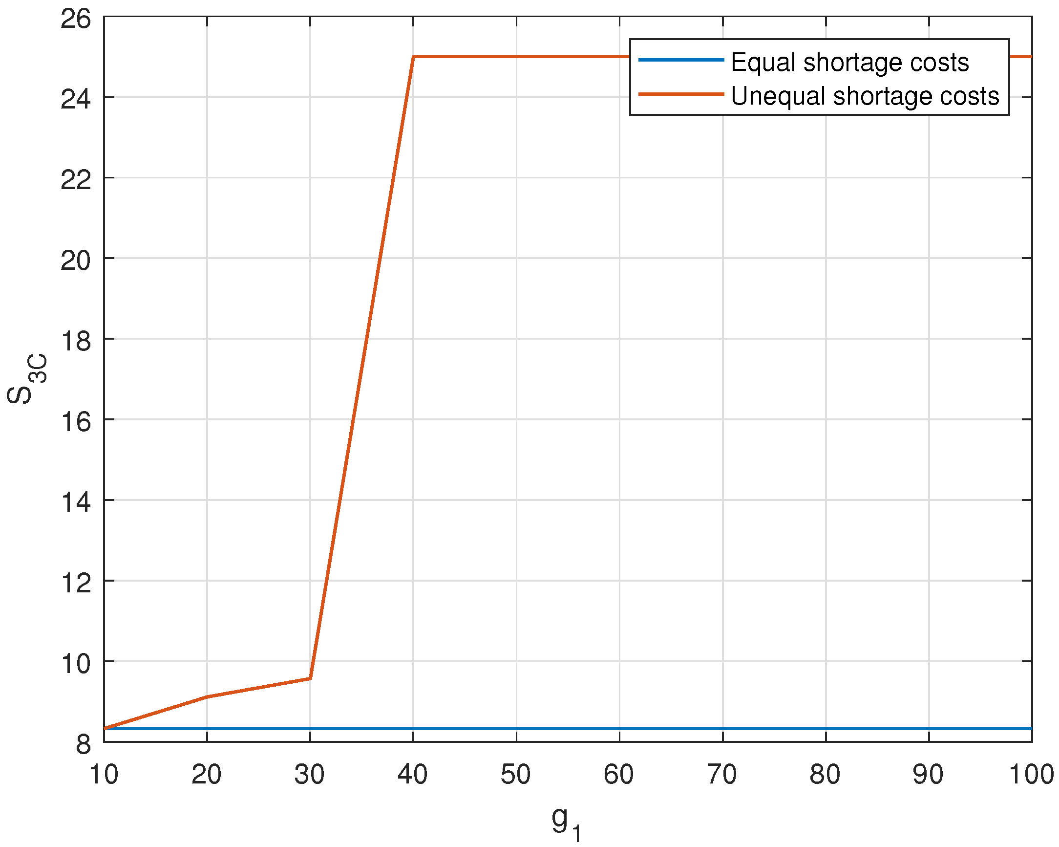
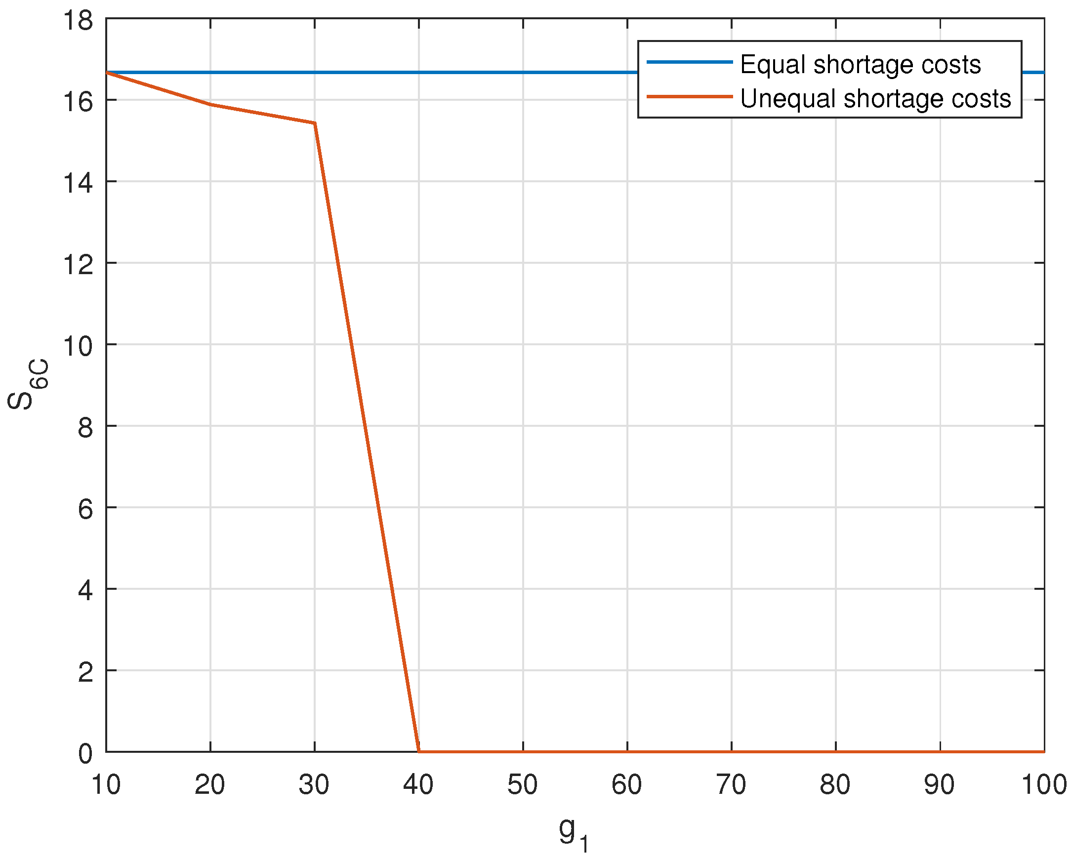
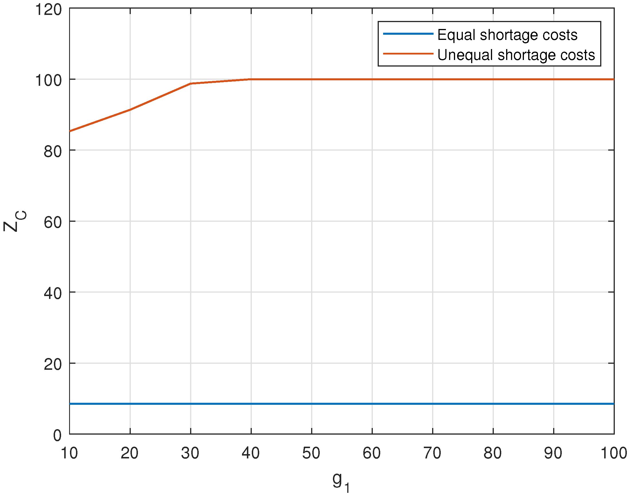
6. Illustrative Examples
Effect of
7. Managerial Aspects and Implications
- The commonality of the components to remanufacturing the products reduces the inventory carrying cost. The quantity and variety of the parts to be kept and maintained in the warehouse reduces to a greater extent as compared to non-commonality of the parts and components. This will significantly improve the commercial viability of a firm as inventory carrying cost will be reduced to a greater extent.
- The movement of the common components would also be faster as most of the products would be using the same component. Thus, the probability of an item becoming dead stock becomes negligible even if some products of the product line of a firm are not in high demand.
- If no commonality, then inventory management and control shall require extra efforts and different means. That further results into more difficulty in managing components and extra cost. Thus, commonality can provide a competitive edge to a firm in the era of globalization.
- The commonality of the components can reduce the requirement of extra inventory. This may boost the manufacturing companies to implement the concept of “Just-in-Time”, which may further result into extra profit margins to a firm.
- The shortage of common components can block the production of many products. The commonality of an item thus may result in higher shortage cost. This paper has tried to find out this shortage impact on any manufacturing firm. This impact may further be extended to the service industry. The shortage of any common component is difficult to afford. Thus, the common component becomes the critical component for the firm.
- This research paper has tried to find out some measures and solutions to the shortage problem with the help of quantitative techniques. This paper is able to develop a mathematical solution to achieve the desired objectives of maximum commonality of items and minimal inventory of components. Thus, it takes the manufacturing firm to a better position of efficient management and control of its inventory.
- Technical, precise, and high accuracy components should not be made common for many final products. If something goes wrong with the common component, it could affect the production of many finished products. Since the chances of design error in simple components is lower, it can be afforded to make simple components common.
8. Conclusions
Author Contributions
Acknowledgments
Conflicts of Interest
References
- Ahmadi, M.; Shavandi, H. Dynamic pricing in a production system with multiple demand classes. Appl. Math. Model. 2015, 39, 2332–2344. [Google Scholar] [CrossRef]
- Teng, H.-M.; Hsu, P.-H.; Wee, P.-H. An optimization model for products with limited production quantity. Appl. Math. Model. 2015, 39, 1867–1874. [Google Scholar] [CrossRef]
- Sarathi, G.P.; Sarmah, S.P.; Jenamani, M. An integrated revenue sharing and quantity discounts contract for coordinating a supply chain dealing with short life-cycle products. Appl. Math. Model. 2014, 38, 4120–4136. [Google Scholar] [CrossRef]
- Yu, Y.; Zhu, J.; Wang, C. A newsvendor model with fuzzy price-dependent demand. Appl. Math. Model. 2013, 37, 2644–2661. [Google Scholar] [CrossRef]
- Abdel-Malek, L.L.; Otegbeye, M. Separable programming/duality approach to solving the multi-product newsboy/gardener problem with linear constraints. Appl. Math. Model. 2013, 37, 4497–4508. [Google Scholar] [CrossRef]
- Pezeshki, Y.; Jokar, M.R.A.; Baboli, A.; Campagne, J.P. Coordination mechanism for capacity reservation by considering production time, production rate and order quantity. Appl. Math. Model. 2013, 37, 8796–8812. [Google Scholar] [CrossRef]
- Rutenberg, D.P. Design commonality to reduce multi-item inventory: Optimal depth of a product line. Oper. Res. 1969, 19, 491–509. [Google Scholar] [CrossRef]
- Rutenberg, D.P.; Shaftel, T. Product design: Subassemblies for multiple markets. Manag. Sci. 1971, 18, 220–231. [Google Scholar] [CrossRef]
- Wickenberg, J.; Stamlin, R.; Persson, M.; Borjesson, S. Challenges for increasing component commonality in platforms. In Proceedings of the EuroMOT, Tampere, Finland, 19–20 September 2011. [Google Scholar]
- Chern, C.-C.; Yang, I.-C. A heuristic master planning algorithm for supply chains that consider substitutions and commonalities. Expert Syst. Appl. 2011, 38, 14918–14934. [Google Scholar] [CrossRef]
- Bernstein, F.; Kök, A.G.; Xie, L. The role of component commonality in product assortment decisions. Manuf. Serv. Oper. Manag. 2011, 13, 261–270. [Google Scholar] [CrossRef]
- Subramanian, R.; Ferguson, M.E.; Toktay, L.B. Remanufacturing and the component commonality decision. Prod. Oper. Manag. 2013, 22, 36–53. [Google Scholar] [CrossRef]
- Alizon, F.; Shooter, S.B.; Simpson, T.W. Improving an existing product family based on commonality/ diversity, modularity, and cost. Des. Stud. 2007, 28, 387–409. [Google Scholar] [CrossRef]
- Lin, Y.; Ma, S.; Liu, L. A multi-period inventory model of component commonality with lead time. In Proceedings of the IEEE International Conference on Service Operations and Logistics, and Informatics, Shanghai, China, 21–23 June 2006; pp. 352–357. [Google Scholar]
- Kranenburg, A.A.; Van Houtum, G.J. Effect of commonality on spare parts provisioning costs for capital goods. Int. J. Prod. Econ. 2007, 108, 221–227. [Google Scholar] [CrossRef][Green Version]
- Wazed, M.A.; Ahmed, S.; Yusoff, N. Impacts of common components on production system in an uncertain environment. Sci. Res. Essay 2009, 4, 1505–1517. [Google Scholar]
- Eynan, A.; Rosenblatt, M.J. The impact of component commonality on composite assembly policies. Nav. Res. Logist. 2007, 54, 615–622. [Google Scholar] [CrossRef]
- Song, J.-S.; Zhao, Y. The value of component commonality in a dynamic inventory system with lead times. Manuf. Serv. Oper. Manag. 2009, 11, 493–508. [Google Scholar] [CrossRef]
- Nonås, S.L. Finding and identifying optimal inventory levels for systems with common components. Eur. J. Oper. Res. 2009, 193, 98–119. [Google Scholar] [CrossRef]
- Boysen, N.; Scholl, A. A general solution framework for component-commonality problems. BuR Bus. Res. 2009, 2, 86–106. [Google Scholar] [CrossRef]
- Jans, R.; Degraeve, Z.; Schepens, L. Analysis of an industrial component commonality problem. Eur. J. Oper. Res. 2008, 186, 801–811. [Google Scholar] [CrossRef]
- Altfeld, N.; Hinckeldeyn, J.; Kreutzfeldt, J.; Gust, P. Impacts on supply chain management through component commonality and postponement: A case study. In Proceedings of the International MultiConference of Engineers and Computer Scientists, Hong Kong, China, 16–18 March 2011. [Google Scholar]
- Labro, E. The cost effect of component commonality. Manuf. Serv. Oper. Manag. 2004, 6, 358–367. [Google Scholar] [CrossRef]
- Fixson, S.K. Modularity and commonality research: Past developments and future opportunities. Concurr. Eng. 2007, 15, 85–111. [Google Scholar] [CrossRef]
- Wazed, M.A.; Ahmed, S.; Yusoff, N. Commonality models in manufacturing resources planning: State-of-the-art and future directions. Eur. J. Sci. Res. 2008, 23, 421–435. [Google Scholar]
- Wazed, M.A.; Ahmed, S.; Yusoff, N. A review of manufacturing resources planning models under different uncertainties: State-of-the-art and future directions. S. Afr. J. Ind. Eng. 2010, 21, 17–33. [Google Scholar] [CrossRef]
- Deflem, Y.; van Nieuwenhuyse, I. Optimal pooling of inventories with substitution: A literature review. Rev. Bus. Econ. 2011, 56, 345–374. [Google Scholar] [CrossRef]
- Baker, K.R.; Magazine, M.J.; Nuttle, H.L.W. The effect of commonality on safety stocks in a simple inventory model. Manag. Sci. 1986, 32, 982–988. [Google Scholar] [CrossRef]
- Gerchak, Y.; Magazine, M.J.; Gamble, A.B. Component commonality with service level requirements. Manag. Sci. 1988, 34, 753–760. [Google Scholar] [CrossRef]
- Eynan, A.; Rosenblatt, M.J. Component commonality effects on inventory costs. IIE Trans. 1996, 28, 93–104. [Google Scholar] [CrossRef]
- Eynan, A. The impact of demands’ correlation on the effectiveness of component commonality. Int. J. Prod. Res. 1996, 34, 1581–1602. [Google Scholar] [CrossRef]
- Jönsson, H.; Silver, E.A. Optimal and heuristic solutions for a simple common component inventory problem. Eng. Costs Prod. Econ. 1989a, 16, 257–267. [Google Scholar]
- Jönsson, H.; Silver, E.A. Common component inventory problems with a budget constraint: Heuristics and upper bounds. Eng. Costs Prod. Econ. 1989b, 18, 71–81. [Google Scholar]
- Jönsson, H.; Jornsten, K.; Silver, E.A. Application of the scenario aggregation approach to a two-stage stochastic, common component inventory problem with a budget constraint. Eur. J. Oper. Res. 1993, 68, 196–211. [Google Scholar] [CrossRef]
- Fu, H.; Fong, D.K.H. A note on the convexity of the objective function for a simple common component inventory problem. Int. J. Prod. Econ. 1998, 55, 143–148. [Google Scholar] [CrossRef]
- Fong, D.K.H.; Fu, H.; Li, Z. Efficiency in shortage reduction when using a more expensive common component. Comput. Oper. Res. 2004, 31, 123–138. [Google Scholar] [CrossRef]
- Fu, H.; Ramasesh, R.; Fong, D.K.H. Component commonality and shortage reduction under a mixed Erlang distributed demand. Int. J. Oper. Res. 2006, 3, 36–46. [Google Scholar]
- Deza, A.; Huang, K.; Liang, H.; Wang, X.J. On component commonality for periodic review assemble-to-order systems. Ann. Oper. Res. 2018, 265, 29–46. [Google Scholar] [CrossRef]
- Rockafellar, R.T. Augmented Lagrangians and applications of the proximal point algorithm in convex programming. Math. Oper. Res. 1976, 1, 97–116. [Google Scholar] [CrossRef]
- Moreau, J.J. Proximité et dualité dans un espace de Hilbert. Bulletin de la Société Mathématique de France 1965, 93, 273–299. [Google Scholar] [CrossRef]
- Martinet, B. Algorithmes pour la Résolution de Problèmes d’Optimisation et de Mini-Max. Thèse d’Etat, Université de Grenoble, Grenoble, France, 1972. [Google Scholar]
- Rockafellar, R.T. The multiplier method of Hestenes and Powell applied to convex programming. J. Optim. Theory Appl. 1973, 12, 555–562. [Google Scholar] [CrossRef]
- Hestenes, M.R. Multiplier and gradient methods. J. Optim. Theory Appl. 1969, 4, 303–320. [Google Scholar] [CrossRef]
- Powell, M.J.D. A Method for Nonlinear Constraints in Minimization Problems; Fletcher, R., Ed.; Academic Press: New York, NY, USA, 1969. [Google Scholar]
- Buys, J.D. Dual Algorithms for Constrained Optimization Problems. Ph.D. Thesis, University of Leiden, Leiden, The Netherlands, 1972. [Google Scholar]
- Luenberger, D.G. Introduction to Linear and Nonlinear Programming, 2nd ed.; Addison-Wesley: Boston, MA, USA, 1984. [Google Scholar]
- Rockafellar, R.T. A dual approach to solving nonlinear programming problems by unconstrained optimization. Math. Program. 1974a, 5, 354–373. [Google Scholar] [CrossRef]
- Rockafellar, R.T. Augmented Lagrange multiplier function and duality in non convex programming. SIAM J. Control 1974b, 12, 268–285. [Google Scholar] [CrossRef]
- Arrow, K.J.; Gould, F.J.; Howe, S.M. A general saddle point result for constrained optimization. Math. Program. 1973, 5, 225–234. [Google Scholar] [CrossRef]
- Bertsekas, D.P. On the method of multipliers for convex programming. IEEE Trans. Autom. Control 1973, AC 20, 385–388. [Google Scholar] [CrossRef]


| Author(s) | Number of Products | Demands Distributions | Common Component | Cost Function |
|---|---|---|---|---|
| Baker et al. [28] | two | independent uniform | all costs equal | max service measure |
| Gerchak et al. [29] | arbitrary | any joint distribution | all costs equal | max expected profit |
| Eynan & Rosenblatt [30] | two | independent uniform | more expensive | min inventory costs |
| Eynan [31] | two | correlated uniform | all costs equal | min inventory costs |
| Jönsson & Silver [32] | two | independent normal | all costs equal | min expected units shortage |
| Jönsson & Silver [33] | arbitrary | independent discrete | all costs equal | min expected units shortage |
| Fu & Fong [35] | two | independent continuous | all costs equal | min expected units shortage |
| Fong et al. [36] | two | independent Erlang | more expensive | min expected units shortage |
| Fu et al. [37] | two | mixed independent Erlang | more expensive | min expected units shortage |
| Unit Shortage Costs | Model C | Model N | ||||
|---|---|---|---|---|---|---|
| 8.3333 | 16.6667 | 8.5318 | 5.2310 | 19.7690 | 0.3868 | |
| 9.1207 | 15.8793 | 91.3565 | 6.1513 | 18.8487 | 4.8524 | |
| Shortage Cost | 10 | 20 | 30 | 40 | 50 | 60 | 70 | 80 | 90 | 100 |
|---|---|---|---|---|---|---|---|---|---|---|
| % gain of | 0.00 | 3.56 | 5.64 | 7.11 | 8.25 | 9.18 | 9.97 | 10.65 | 11.25 | 11.79 |
| % reduction of | 0.00 |
© 2019 by the authors. Licensee MDPI, Basel, Switzerland. This article is an open access article distributed under the terms and conditions of the Creative Commons Attribution (CC BY) license (http://creativecommons.org/licenses/by/4.0/).
Share and Cite
Hamdi, A.; Tadj, L. Augmented Lagrangian Approach to the Newsvendor Model with Component Commonality. Math. Comput. Appl. 2019, 24, 55. https://doi.org/10.3390/mca24020055
Hamdi A, Tadj L. Augmented Lagrangian Approach to the Newsvendor Model with Component Commonality. Mathematical and Computational Applications. 2019; 24(2):55. https://doi.org/10.3390/mca24020055
Chicago/Turabian StyleHamdi, Abdelouahed, and Lotfi Tadj. 2019. "Augmented Lagrangian Approach to the Newsvendor Model with Component Commonality" Mathematical and Computational Applications 24, no. 2: 55. https://doi.org/10.3390/mca24020055
APA StyleHamdi, A., & Tadj, L. (2019). Augmented Lagrangian Approach to the Newsvendor Model with Component Commonality. Mathematical and Computational Applications, 24(2), 55. https://doi.org/10.3390/mca24020055