Article

Modeling and Simulation of a Hydraulic Network for Leak Diagnosis

1
TURIX-Dynamics Diagnosis and Control Group, Tecnológico Nacional de México, Instituto Tecnológico de Tuxtla Gutiérrez, Tuxtla Gutiérrez 29050, Mexico
2
GIPSA-lab, CNRS, Grenoble INP, Université Grenoble Alpes, 38000 Grenoble, France
3
Tecnológico Nacional de México, Instituto Tecnológico de Hermosillo, Hermosillo 83170, Mexico
4
Cátedras CONACYT, Instituto de Ingeniería, Universidad Nacional Autónoma de México, Ciudad de México 04510, Mexico
*
Authors to whom correspondence should be addressed.
Math. Comput. Appl. 2018, 23(4), 70; https://doi.org/10.3390/mca23040070
Submission received: 28 September 2018 / Revised: 4 November 2018 / Accepted: 4 November 2018 / Published: 6 November 2018
(This article belongs to the Special Issue Optimization in Control Applications)

Abstract

:
This work presents the modeling and simulation of a hydraulic network with four nodes and two branches that form a two-level water distribution system. It also proposes a distribution of hydraulic valves that allows emulating a leak using a valve and different network configurations, e.g., simple ducts, closed networks and branched networks. The network is modeled in the steady state considering turbulent flow. Numerical experiments are performed, and the results show that the proposed network is useful for the design of leakage diagnosis and control algorithms in different configurations and leakage scenarios.

1. Introduction

Safety and proper functioning of hydraulic networks are very important, since these systems are used in the industrial and governmental sectors for the transportation of different types of fluids such as gases, hydrocarbons and water. In this sense, one of the main problems in the distribution networks of liquids are hydraulic leaks, where a hydraulic leak is defined as the uncontrolled output of fluid that occurs in any section of the network. A leak can occur when there is corrosion on the inside or outside of the pipe, or it can be caused by blows, by the theft of transported product, etc. [1]. Leaks have serious consequences such as environmental pollution, economic losses and human deaths from hydrocarbon explosions. Leaks occur more frequently in worn pipes, pipes with low maintenance, pipe joints or in some accessories such as elbows and valves, among others [2].
Due to the strong environmental and social impact caused by leaks in water distribution systems, it is necessary to reduce this problem [3], taking into account that the water demands increase as the population multiplies, and water losses in highly populated cities increase in a high percentage as well. The Organization for Economic Cooperation and Development (OECD) conducted a survey in 42 cities with the highest leakage problem in their distribution networks. In the list, one can find Mexican cities like Tuxtla Gutiérrez with a flow loss of 70%, San Luis Potosí with 50% and Mexico City with more than 40%. Other important cities around the world are Paris with loses of 10%, Hong Kong (China) with more than 15% and Liverpool with more than 20% [4]. These percentages of water losses in distribution networks give evidence of the need to develop solutions in order to solve or at least mitigate this problem.
Different works have been developed that focus on leak detection and control of hydraulic network systems. For example, Van Pham et al. [5] used a receding horizon optimal control method applied to the flow model of the network, guaranteeing the convergence of pressures in case of transients; Torres et al. [6] designed a state observer through redundant relationships in order to isolate sensor and actuator faults and unknown extractions of fluid; Wang et al. [7] used a robust predictive control algorithm to control pressures and flows in the demanding nodes in a small network. In order to validate these algorithms, it is necessary to test them experimentally in laboratory plants that can reproduce, at scale, the behavior of real hydraulic networks. In this context, different pilot plants have been built for experimentation with emphasis on hydraulic leaks. For example, at the laboratory of the Engineering Institute of UNAM(Mexico), a hydraulic network was designed with a vertical coil arrangement where leak detection and localization algorithms have been developed using model- and data-based techniques using monitoring software in Labview® and MATLAB® for flow and pressure analysis [8,9]. In the hydraulic laboratory at CINVESTAVcampus Guadalajara (Mexico), the pilot plant has a rectangular geometry, and it has also enabled the development of leak detection algorithms with model-based methods [10,11]. GIPSA-lab (France) and the University of Catalonia (Spain) also have facilities enabling the experimentation with hydraulics networks [7,12], and the list can continue. On the other hand, when there are no pilot plants available or the physical extension of the hydraulic network is prohibitive for a laboratory, it is necessary to use specialized software to emulate the behavior of the network. One of these software programs is EPANET®, which is a public domain, water distribution system modeling software package developed by the United States Environmental Protection Agency; it performs extended-period simulation of hydraulic and water-quality behavior within pressurized pipe networks, and it has been also used for leak detection [13]. Flow-Master® is another software program that has been used for the representation of hydraulic networks and the development of leakage detection and localization techniques [14].
In line with the laboratories previously mentioned, as well as their important usefulness in the development of new leak detection and localization techniques, this paper proposes a model of an extended hydraulic network with two lateral connections that is under construction at the Instituto Tecnológico de Tuxtla Gutiérrez. It will allow experimenting with a hydraulic network of a few nodes that emulate some real problems that arise in a real distribution network. Therefore, this work presents the modeling and simulation of a 200 m hydraulic network, with a storage depot of 2500 L, a hydraulic pump of 5 hp, four nodes in its two lateral sockets and valves for the simulation of leaks. SolidWorks® is used to present its geometric arrangement in order to consider the space available at the laboratory where it will be located. The physical layout of the network consists of a base with two lateral branches that connect to a second level. The steady-state model of the hydraulic network obtained in the MATLAB® environment is also described. In this way, a unique prototype that simulates a real hydraulic network is obtained. It will serve as an experimental basis to develop leakage diagnosis algorithms, in addition to optimal control techniques applied to the network to reduce water waste due to hydraulic leaks. The results are presented with the description of the parameters obtained in leak-free and leak conditions.

2. Modeling of the Hydraulic Network

2.1. Hydraulic Concepts

A distribution network comprises a collection of interconnected pipe sections in a specific configuration, each one with a length, a diameter and a roughness according to the material. Sections of the pipeline may contain pumps and accessories, such as elbows and valves. The end points of each pipe section are identified as union nodes or fixed grade nodes. A joint node is a point where two or more sections of pipe join together, and it is also a point of consumption where the flow can enter and exit the system. A node of fixed degree is a point where a constant piezometric height is maintained, such as a connection to a reservoir, an elevated storage tank or any other constant pressure region. In any pipe network, the following equation is fulfilled [15]:
N P = N J + N L + N F 1 ,
where N P is the number of pipe sections (also called lines), N J is the number of union nodes, N L is the number of closed loops and N F is the number of fixed degree nodes.
On the other hand, hydraulic pumps can be described in several ways. For some applications, a constant power input is specified. For other applications, a curve is adapted to the actual operating data of the pump. For pumps described for their useful power P u , the energy added by the pump between the nodes i , j is expressed in terms of the flow rate by:
H j H i = μ P u / Q i j ;
where H is the pressure head (mwc), μ it is a constant that depends on the units used and Q is the flow (m3/s). Alternatively, a pump can be described by its flow values at different operating points; these points relate the discharges (output flows) with the differences in piezometric height through the pump. A quadratic polynomial can be adjusted through these points to obtain a characteristic curve that describes the operation of the pump in the form:
H j H i = a 0 η 2 + b 0 η Q i j + c 0 Q i j 2 ,
where a 0 , b 0 y c 0 are the coefficients of the curve that represent the real operation when the pump works at maximum speed. At least three data points are required to determine the coefficients, where η is the proportion of the rotational speed at any time, with respect to the rotational speed associated with the data used to determine the coefficients [16].

2.2. Energy Losses and Mass Balance in Hydraulic Networks

When there is fluid transport in a hydraulic network, an advance resistance is generated due to the roughness of the material, where the relative roughness is defined by:
ϵ = k s / d ,
where k s is the absolute roughness (mm) and d is the diameter of the pipeline (mm). Another important parameter of the flow in hydraulic networks is the friction factor f, which depends on the geometry of the pipe and the Reynolds number (Re). The friction factor depends on the flow turbulence, which is considered to be laminated when Re < 2000 , and it is considered turbulent when Re > 4000 [17]. In a turbulent regime, the friction factor depends not only on the Reynolds number, but also on the relative roughness ( ϵ ). In the transition region 2000 Re 4000 , to estimate the friction, a cubic interpolation is made with the border values of both regimes. Taking into account both types of flow (laminar and turbulent), the friction factor is calculated with:
f = 64 / Re , Re < 2000 ; 2 log 10 ϵ 3.7 + 5.74 Re 0.9 2 , Re > 4000 .
When the system is in a steady state, it is possible to calculate the friction factor with the Darcy–Weisbach equation using measurements obtained from the hydraulic network, to next use the Colebrook equation to calculate the roughness coefficient of the hydraulic network material. However, in practice, an explicit approximation using the Swamee–Jain equation is used [18]:
f = 0.25 log 10 ε 3.7 + 5.74 Re 0.9 2 .
Therefore, considering the roughness of the material and the friction caused by the flow through the pipeline, the pressure energy losses are defined by the Darcy–Weisbach equation:
H i H j = h i j = f L Q i j 2 / 2 g A 2 d ,
where L is the length (m) of the pipeline, h i j is the loss of pressure (mwc) when the flow passes through the pipe, A is the area of the cross-section ( m 2 ) of the pipeline, d is the diameter of the pipeline (mm) and g is the gravity (m/s2). It is possible to represent some parameters of the Darcy–Weisbach equation in a single coefficient of the form:
r i j = f L / 2 g A 2 d ,
and Equation (7):
H i H j = h i j = r i j Q i j 2 ,
where r i j is the coefficient of resistance to flow. It is important to mention that the equivalent length of the accessories in the hydraulic network is included in the variable L of Equation (8).
For the flows that are distributed in hydraulic networks, the principle of the conservation of mass in each node of the hydraulic network is considered, and it is presented in the following equation:
i Q i j = D j ,
where the sum considers all the flows arriving at the node j from any adjacent node i and D j is the demand or consumption in the node j. On the other hand, to represent a leak at any point of the hydraulic network, the Torricelli equation is used [19]:
Q f = λ f H f ,
where Q f it is the flow of the leak, λ is the leakage coefficient and H f is the pressure at the point where the leak occurs. The leakage coefficient is calculated according to the following expression:
λ f = c d A d 2 g ,
where c d is a discharge coefficient in the leak and A d is the area of the hole in the pipe where the leak occurs. These equations are considered in the modeling of hydraulic networks.
In this case, the model developed is in the steady state regime in order to guarantee flow in all regions of the hydraulic network even when a leakage flow is present at any point in the pipeline. The leak, in this case, is modeled with Torricelli’s equation. However, it is important to mention that in a real hydraulic network system, the flow regime is normally turbulent, which means that a more accurate model is needed to consider the transient effects in order to perform a pressure wave analysis in the case of an abrupt leak.
In the design of the hydraulic network, the Schedule 80 PVC pipe is proposed for its elastic properties and low cost compared to other materials. Other characteristics of the network, such as the inner diameter, the length of the pipe and the coil arrangement of the system were proposed according to the available space in the hydraulic laboratory. The diameter and length are physical parameters that are directly considered in the model. In the case of the coil arrangement and elbows, these are used to redirect the flow, causing more turbulence and more energy losses. However, the energy losses caused by accessories are included indirectly by considering an equivalent straight pipe with that energy loss.

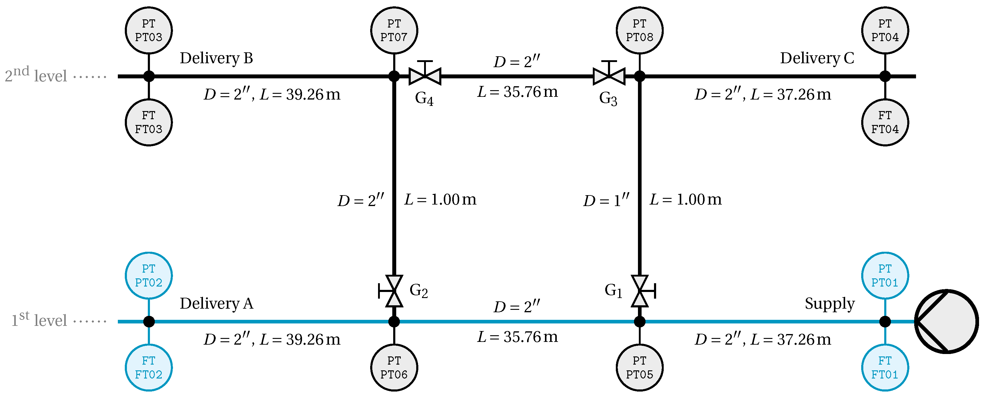
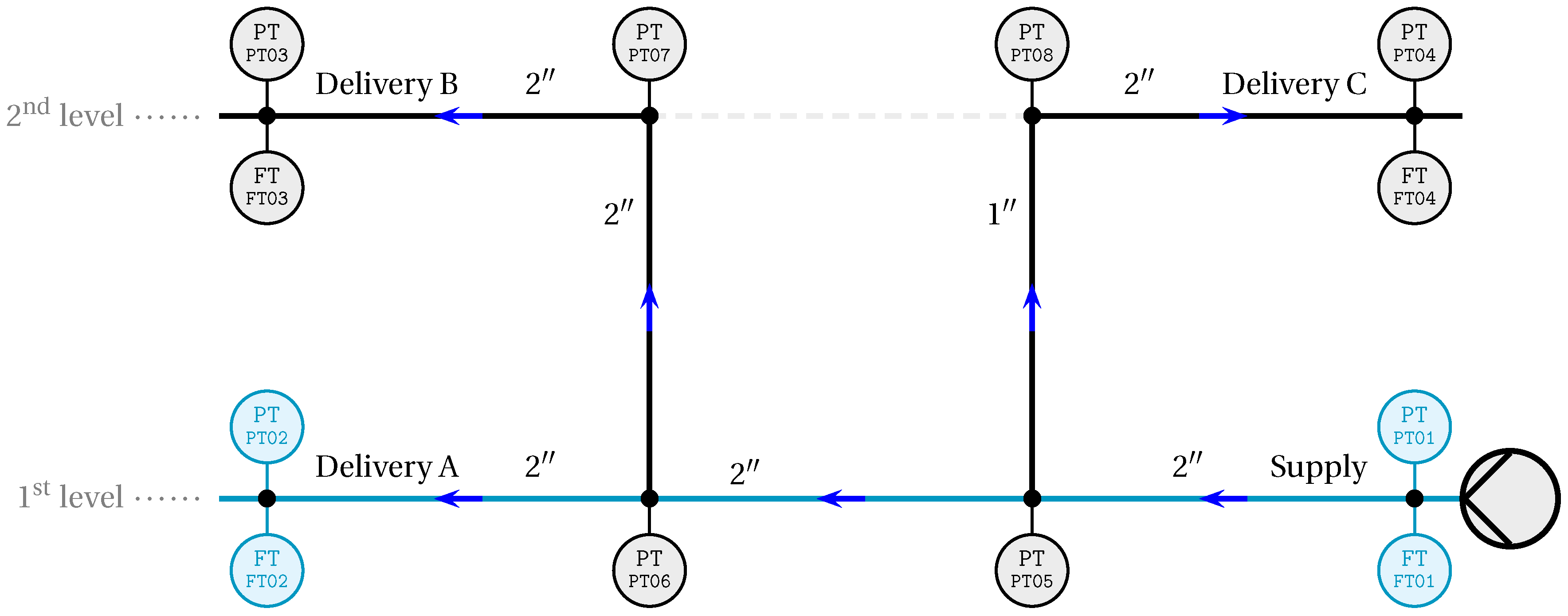
2.3. Configurations of the Proposed Hydraulic Network

The proposed hydraulic network is designed to represent three geometric arrangements; this is possible according to the opening and closing of valves distributed in the system. The first configuration is represented in the instrumentation diagram of Figure 1, where all the valves remain open. The second configuration is achieved by closing valves G1 and G2, to get the shape of a simple pipe, as presented in Figure 2. Finally, the third configuration consist of a duct with two branches, which can be obtained when the valves G3 and G4 are closed, leading to the arrangement shown in Figure 3. This emphasizes that the proposed hydraulic network is reconfigurable, and it will allow the development of leak detection and control algorithms in hydraulic networks with different topologies. The physical layout of the hydraulic network (as it will be at the end of its construction) is shown in Figure 4. The first level of this hydraulic network is already built and instrumented [20] and the construction of the second level is work in process that should be completed by the end of 2018.
The importance of the different configurations of the proposed network is because they represent real cases of hydraulic distribution networks. For example, the configuration of a single pipeline is commonly used in hydrocarbon distribution networks where the fluid is transported by very extensive (kilometers of) single pipelines; the branched network is commonly used to transport fluids in industry, where there is a single source/reservoir of fluid and several demand points at different ends of the network; while the interconnected network (closed network) is used in the transport of drinkable water, allowing, in some cases, the water supply of a complete city.

2.4. Modeling of the Proposed Hydraulic Network

Figure 5 shows the pressures on the nodes and the directions of the flows through the hydraulic network, as well as the nomenclature considered to develop the mathematical model of the network.
To model the hydraulic network, it is necessary to apply the energy loss equations in each line or pipe of the system and a mass balance in each node.
On the other hand, as was previously mentioned, the lower level of the network is a section already built and instrumented at the Instituto Tecnológico de Tuxtla Gutiérrez (ITTG) hydraulics laboratory. The piezometric height values are known according to the water level of the deposit (where the flow is stored and recirculated to flow into the network). Furthermore, the pressure provided by the pump is known through sensors at the first level of the network, and it is considered as the boundary parameter that causes the flow in the network. These are known values in the system of equations that models the proposed network and that will be solved simultaneously. The known parameters include the pressures H 0 , H 4 , H 5 , H 8 referring to the nodes of Figure 5, which conform to 1 mwc, and as for Node 1 of the hydraulic pump H 1 , the values are according to the characteristic curve generated by a pressure of 5.60 mwc and a flow of 3.83 m3/s, while the roughness value of the Schedule 80 PVC material is ϵ = 0.0235 mm, calculated with the Swamee–Jain equation with the experimental values obtained from the simple duct configuration that was already built [20]. The proposed lengths and diameters in each region of the network are presented in Table 1. Using Equations (3), (9) and (11), a system of nonlinear equations is obtained that will be solved in MATLAB®, where it is possible to assign different values arbitrarily to the leakage coefficient λ to simulate different scenarios without leakage and with leakage in Node 9, which represents a hole that introduces to the model a virtual node between Nodes 2 and 3. In this way, the pressure and flow values distributed throughout the hydraulic network will be obtained. Therefore, from the system represented in Figure 5, the next set of equations is generated; for pressure drops in the system, the model is presented as follows,
H 0 H 1 = F ( Q p u m p ) ,
H 1 H 2 = r 12 Q 12 2 ,
H 2 H 9 = r 29 Q 29 2 ,
H 3 H 4 = r 34 Q 34 2 ,
H 2 H 6 = r 26 Q 26 2 ,
H 6 H 5 = r 65 Q 65 2 ,
H 6 H 7 = r 67 Q 67 2 ,
H 7 H 8 = r 65 Q 65 2 ,
H 3 H 7 = r 37 Q 65 2 ,
H 9 H 3 = r 93 Q 93 2 ,
where the coefficient r i j is described in Equation (8) and F indicates that the pressure difference between Nodes 0 and 1 of the network is a function of the flow produced by the pump.
Considering the mass balance in the nodes of the system, the following set of equations is obtained,
Q p u m p Q 12 = 0 ,
Q 12 Q 29 = Q 26 ,
Q 29 Q l e a k = Q 93 ,
Q 93 Q 34 = Q 37 ,
Q 26 Q 65 = Q 67 ,
Q 37 + Q 67 = Q 78 ,
where the leakage flow is calculated with the Torricelli Equation (11):
Q l e a k = λ H 9 .

3. Numerical Experiments

The set of Equations (13)–(29) obtained in the previous section is solved in MATLAB® using the nonlinear optimization method called “trust region”, whose purpose is to solve a system of equations f ( x ) = 0 in order to find the optimal solution through an iterative process minimizing f ( x ) 2 . The efficiency of this numerical method is due to its rapid convergence [21]; in fact, it only takes 3–5 s to simulate, on a PC with a Core i5 processor, 24 h of running time.
The first numerical experiment is performed in the closed network without leaks. The solution of the model provided the values of flow and pressure in different regions of the hydraulic network. The results are shown in Figure 6 where the pressure values (mwc) are located at the nodes and the flows (m3/s) in the lines of the figure. The pressure values at the ends of the hydraulic network (Nodes 0, 4, 5, 8) are known values with a hydraulic height of 1 mwc. This height corresponds to the water reservoir, as there will be a single deposit that will be used to supply, store and demand water to/from the network. Therefore, all the network ends connect to this deposit, and the water is recirculated through the system. It also should be noted here that the displayed pressure values are gauge pressure values, i.e., zero-referenced against ambient air pressure, so they are equal to absolute pressure minus atmospheric pressure.
In the same way, a second numerical experiment is performed considering a leak in Node 9 at a z distance with respect to Node 0; the obtained values are presented in Figure 7. In this case, the results show that, when a leak occurs, the pressures decrease in each node of the network, and there are variations in the flow rates. The leak was proposed in Node 9; however, if the leak is in any other region of the pipe, new values of flows and pressures would be obtained in the network due to the mass and energy conservation, respectively. However, the flow in each section of the hydraulic network is still turbulent considering its speed and its diameters with respect to the Reynolds number.
The numerical experiment whose result is shown in Figure 7 corresponds to a specific and unique leakage configuration. However, using the mathematical model of the network, it is possible to simulate varying conditions over time, e.g., programmed consumptions in the nodes that change during the day or leaks that increase progressively, among others. To execute these numerical experiments—called “extended period” in the specialized literature—from the steady state equations, a sweep is made of the values that the parameters can take over time using “for” cycles, as shown in the following pseudocode:
params = value_list;sols = [];for param = params sol = simulateNetwork(param); sols = [sols,sol];end
With the previous consideration, the network was simulated with a progressive leak in Node 9, and the gradual change in the leak coefficient was modeled using an exponential function:
λ = 1 × 10 4 1 exp ( t × 3600 / 3 ) [ m 5 / 2 s 1 ] ,
where t is time in hours. This function was selected considering that its evolution over time represents an increase from zero to a value λ m a x = 1 × 10 4 that would correspond to a leak through a circular hole of about a quarter of an inch in diameter. In the graphs of Figure 8 and Figure 9, the effects of a leak over the network are shown, i.e., the increase in the flow rate and the loss of the pressure head at the outlet of the pump. In Figure 8, it can be seen that the flow of the pump Q p u m p represented between Nodes 0 and 1 remains constant over time when the system does not leak; however, this flow increases exponentially when a leak is present in the system.
In relation to the pressure variation in the system due to the occurrence of a leak, in Figure 9, it is appreciated how the pressure H 1 remains constant in the absence of leaks in the system, but decreases when the leak appears.

4. Conclusions

This paper presented the design of a prototype of a hydraulic network that allows the development of leakage control and diagnosis algorithms for three different configurations: single ducts, ducts with branches and closed networks. The proposed hydraulic network was modeled, obtaining its system of equations for the steady state case, which was solved using nonlinear optimization algorithms. Numerical experiments in MATLAB® showed that the proposed network structure guarantees turbulent flow in all its lines for the considered configurations and that its construction and use as a scale model of pressurized networks is feasible. It is important to mention that the developed model is part of a section already built of the hydraulic network, which is the simple pipeline section. The known and experimentally-validated parameters of the already built section of the network were taken into account in the extended model of the network. However, it is necessary to perform a mean square error analysis between the experimental values of flow and pressure and the values obtained numerically to further adjust the parameters of the model. This analysis remains as future work. Finally, the goal of the model was to ensure the description of the flow in all sections of the network, leaving the study of the transitory effects for future work. The inclusion of the transitory effects in the model will allow the extension of the leakage diagnosis and control techniques, as well.

Author Contributions

F.-R.L.-E. and G.V.-P. conceived and designed the experiments; J.-R.B. and H.-R.H. performed the experiments; G.B. and L.T. analyzed the data; J.-R.B. wrote the paper.

Funding

This research was funded by the National Council for Science and Technology (CONACYT) of Mexico, Grant Number PN-2016/3595, and Tecnológico Nacional de México (TecNM) under the program Apoyo a la Investigación Científica y Tecnológica, Grant Number 6358.17-P.

Conflicts of Interest

The authors declare no conflict of interest.

References

  1. Solis Luna, N.B. Determinación Remota de Fugas de Gas y Petróleo Por Medio de Cámaras Infrarrojas. Ph.D. Thesis, Instituto Politécnico Nacional, Mexico City, Mexico, 2009. [Google Scholar]
  2. Fuentes-Mariles, O.; Palma-Nava, A.; Rodríguez-Vázquez, K. Estimación y localización de fugas en una red de tuberías de agua potable usando algoritmos genéticos. Ing. Investig. Techol. 2011, 12, 235–242. [Google Scholar]
  3. Doney, K. Leak Detection in Pipelines Using the Extended Kalman Filter and the Extended Boundary Approach. Ph.D. Thesis, University of Saskatchewan, Saskatoon, SK, Canada, 2007. [Google Scholar]
  4. OECD. Water Governance in Cities. In OECD Studies on Water; OECD: Paris, France, 2016. [Google Scholar]
  5. Van Pham, T.; Georges, D.; Besancon, G. Predictive control with guaranteed stability for water hammer equations. IEEE Trans. Autom. Control 2014, 59, 465–470. [Google Scholar] [CrossRef]
  6. Torres, L.; Verde, C.; Carrera, R.; Cayetano, R. Algoritmos de diagnóstico para fallas en ductos. Techol. Cienc. Agua 2014, 5, 57–78. [Google Scholar]
  7. Wang, Y.; Blesa, J.; Puig, V. Robust Periodic Economic Predictive Control based on Interval Arithmetic for Water Distribution Networks. IFAC-PapersOnLine 2017, 50, 5202–5207. [Google Scholar] [CrossRef] [Green Version]
  8. Verde, C. Multi-leak detection and isolation in fluid pipelines. Control Eng. Pract. 2001, 9, 673–682. [Google Scholar] [CrossRef]
  9. Torres, L.; Besancon, G.; Georges, D. A collocation model for water-hammer dynamics with application to leak detection. In Proceedings of the 47th IEEE Conference on Decision and Control, Cancun, Mexico, 9–11 December 2008; pp. 3890–3894. [Google Scholar]
  10. Navarro, A.; Begovich, O.; Besançon, G.; Dulhoste, J. Real-time leak isolation based on state estimation in a plastic pipeline. In Proceedings of the IEEE International Conference on Control Applications (CCA), Denver, CO, USA, 28–30 September 2011; pp. 953–957. [Google Scholar]
  11. Delgado-Aguiñaga, J.; Besançon, G.; Begovich, O.; Carvajal, J. Multi-leak diagnosis in pipelines based on Extended Kalman Filter. Control Eng. Pract. 2016, 49, 139–148. [Google Scholar] [CrossRef]
  12. Ocampo-Martinez, C.; Barcelli, D.; Puig, V.; Bemporad, A. Hierarchical and decentralised model predictive control of drinking water networks: Application to barcelona case study. IET Control Theory Appl. 2012, 6, 62–71. [Google Scholar] [CrossRef]
  13. Scola, I.R.; Besançon, G.; Georges, D. Optimizing Kalman optimal observer for state affine systems by input selection. Automatica 2018, 93, 224–230. [Google Scholar]
  14. Soldevila, A.; Fernandez-Canti, R.M.; Blesa, J.; Tornil-Sin, S.; Puig, V. Leak localization in water distribution networks using Bayesian classifiers. J. Process Control 2017, 55, 1–9. [Google Scholar] [CrossRef]
  15. Wood, D.J.; Rayes, A.G. Reliability of algorithms for pipe network analysis. J. Hydraul. Div. 1981, 107, 1145–1161. [Google Scholar]
  16. Wylie, E.B.; Streeter, V.L. Hydraulic Transients; FEB Press: Ann Arbor, MI, USA, 1983. [Google Scholar]
  17. Crane. Flujo de Fluidos en Válvulas, Accesorios y Tuberías; McGraw-Hill: New York, NY, USA, 1989. [Google Scholar]
  18. Genić, S.; Aranđelović, I.; Kolendić, P.; Jarić, M.; Budimir, N.; Genić, V. A review of explicit approximations of Colebrook’s equation. FME Trans. 2011, 39, 67–71. [Google Scholar]
  19. Mott, R.L. Mecánica de Fluidos Aplicada; Pearson Educación: Turin, Italy, 1996. [Google Scholar]
  20. Bermúdez, J.R.; Santos-Ruiz, I.; López-Estrada, F.R.; Torres, L.; Puig, V. Diseño y modelado dinámico de una planta piloto para detección de fugas hidráulicas. In Proceedings of the Congreso Nacional de Control Automático CNCA 2017, Mexico City, Mexico, 4–6 October 2017; Asociación Mexicana de Control Automático: Mexico City, Mexico, 2017; Volume 1, pp. 2–7. [Google Scholar]
  21. Coleman, T.F.; Li, Y. An interior trust region approach for nonlinear minimization subject to bounds. SIAM J. Optim. 1996, 6, 418–445. [Google Scholar] [CrossRef]
Figure 1. Complete configuration of the hydraulic network.
Mca 23 00070 g001
Figure 2. Simple pipe configuration.
Mca 23 00070 g002
Figure 3. Sectioned hydraulic network configuration.
Mca 23 00070 g003
Figure 4. Front view of the hydraulic network in SolidWorks®.
Mca 23 00070 g004
Figure 5. Nomenclature of the system variables.
Mca 23 00070 g005
Figure 6. Pressures and flows in the network without leakage.
Mca 23 00070 g006
Figure 7. Pressures and flows in the network with a leakage in Node 9.
Mca 23 00070 g007
Figure 8. Flow variation in the presence of a leak.
Mca 23 00070 g008
Figure 9. Pressure head loss at the pump outlet caused by a leak.
Mca 23 00070 g009
Table 1. Dimensions of the pipe sections.
SectionLength (m)Diameter (mm)
1 2 37.2648.6
2 9 x(*)48.6
9 3 35.76 x 48.6
3 4 39.2648.6
2 6 1.0024.3
3 7 1.0048.6
6 5 37.2648.6
6 7 35.7648.6
7 8 39.2648.6
(*) Denotes an arbitrary escape position between Nodes 2 and 3.

