Applying Computer Algebra Systems in Approximating the Trigonometric Functions

Abstract

We propose numerical algorithms which can be integrated with modern computer algebra systems in a way that is easily implemented to approximate the sine and cosine functions with an arbitrary accuracy. Our approach is based on Taylor’s expansion about a point having a form of $kp$, $k\in \mathbb{Z}$ and $p=\pi /2$, and being chosen such that it is closest to the argument. A full error analysis, which takes advantage of current computer algebra systems in approximating $\pi$ with a very high accuracy, of our proposed methods is provided. A numerical integration application is performed to demonstrate the use of algorithms. Numerical and graphical results are implemented by MAPLE.

1. Introduction

It is an undoubted fact that the design of more reliable and accurate algorithms to compute the approximate values to the sine and cosine functions is one of the most fascinating topics of the constructive approximation of functions. This is clearly motivated by numerous applications of these trigonometric functions ranging from mathematics, physics to engineering.

The use of polynomial approximations plays a key role in computing values of the sine and cosine functions, as well as other elementary functions. The most commonly used polynomials are Taylor, Chebyshev, and Remez. Let us briefly mention an early historical fact related to approximating the trigonometric functions. That is the formula proposed by Bhaskara in the 7th century:

$$\sin ({\theta }^{\circ })\approx \frac{4\theta (180-\theta )}{40500-\theta (180-\theta )},0\le \theta \le 180,$$

which is now explained clearly and logically (see [1]). The explanation is based on the view of interpolation by polynomials and rational functions.

For these days, with a rapid development of technology and computer science, there has been great effort to build hardware and software algorithms for evaluating values of the elementary functions, especially the trigonometric functions, to meet an essential need in scientific computations, signal processing, telecommunication and computer graphics [2]. Among these algorithms is the most important and fundamental one called the CORDIC algorithm. The name CORDIC is an acronym for Coordinate Rotation Digital Computer. This is a computing technique for solving the trigonometric relations that consist of plane coordinate rotation, Cartesian and polar coordinates. Details on CORDIC and developments on algorithms for evaluating elementary functions can be found in the excellent monograph by Muller [3] Chapter 7, and also [4,5,6,7,8].

It is worth mentioning that the desirable accuracy of computed transcendental functions mainly depends on the demand of users and/or practical scientific use. On the one hand, it would usually suffice to numerically solve real-world problems with an accuracy to machine precision. This is the reason that the majority of present computing software programs such as MATLAB, and its Chebfun software package, developed by Trefethen and his team [9], aims to support. On the other hand, there has always been an imperative need to seek for simpler and more efficient algorithms with higher accuracy as the interest in improving scientific calculation method itself or from other sources of practical demand. This is purely our intention when writing the present article. The design and development of our algorithms stem from the fact that we are able to easily work with higher-degree polynomials (even degrees of thousands or millions [10] Chapter 1) due to the increasing complexity of computer applications.

The goals of this paper are twofold. Firstly, we present an algorithm that gives pointwise approximate values of the sine and cosine functions at any rational angle with a desired precision. Secondly, our biggest contribution to novelty is the piecewise approximation procedure with an arbitrary small absolute error applied to these trigonometric functions. To this end, we introduce a special partition that can take the advantage of dividing an interval $[a,b]$ into appropriate subintervals for the approximation process. Our construction is merely based on the lookup table-like storage of approximate values of Pi (the number $\pi$). In some computer algebra systems, we can do this with built-in commands such as evalf[n](Pi) from MAPLE, vpa(pi,n) from MATLAB and N[Pi,n] from MATHEMATICA.

In principle, approximating the value $f(x)=\sin x$ by the Taylor polynomial of order n at a point $x_0$ as

$$f(x)\approx P_n(x)=\sum _{m=0}^n\frac{f^{(m)}(x_0)}{m!}{(x-x_0)}^m$$

is meaningful when the point $x_0$ satisfies $|x-x_0|<1$ and all the coefficients $f^{(m)}(x_0)$ can be explicitly calculated. Such a point can be chosen as $kp$, where $k\in \mathbb{Z}$ and $p=\pi /2$. We will choose k to get the inequality even better $|x-x_0|<0.8$. Because we only have rational approximate values of p, this challenges us with several practical questions to be solved: how to evaluate errors arising from replacing p with its approximate value $p^{\prime }$ and how to keep $f^{(m)}(x_0)$ unchanged with this change of value of p? In addition, we also need an efficient mechanism to access rational approximate values of p more enough to reach an acceptable or desired precision. Fortunately, more and more precise values of Pi have been updated from the projects of computation of special numbers (see [11], for instance), and these values are now supplied conveniently and efficiently for use by present computer algebra systems. The current record of the longest decimal number computed for Pi has been 13.3 trillion digits (date announced: 8 October 2014), held by an anonymous programmer known online as “houkouonch”, and will be certainly broken later.

The paper is organized as follows. In Section 2, we define the steps to obtain Taylor polynomials for approximating values of the sine function with an absolute error less than a given tolerance. We then, in Section 3, provide appropriate regulations to show that it is possible to keep coefficients of the approximate Taylor polynomials unchanged when $p=\pi /2$ is replaced with its approximate value $p^{\prime }$. The error analysis is presented in the same section in which the properties of special functions Gamma and Modified Bessel are used. We arrive at our algorithms for pointwise approximating values of the sine and cosine functions, and for piecewise approximating on any interval $[a,b]$ in Section 4 and Section 5. To demonstrate the performance of our methods, Section 6 is devoted to an application of numerical integration. Finally, some concluding remarks are discussed in the last section. For our purpose, we use MAPLE to implement our algorithms, and demonstrate numerical and graphical results.

2. Formulation

Recall that the function $f(x)=\sin x$ is periodic with period $2\pi$, differentiable of any order, and for each $k_0\in \mathbb{Z}$ and $m=0,1,\dots$, we have

$$f^{(m)}(k_0\pi /2)=\left\{\begin{array}{cc}0,& m+k_0=2k,\hfill \\ {(-1)}^k,& m+k_0=2k+1(k\in \mathbb{Z}).\hfill \end{array}\right.$$

(1)

Given a number x, we can choose an integer k such that $k\pi /2\le x<(k+1)\pi /2$, which is $k=\lfloor x/p\rfloor$ (here, we denote $\pi /2$ by p, for brevity, and $\lfloor z\rfloor$ is the integral part of a number z). Now, we determine $k_0\in \mathbb{Z}$ by an if-then statement: if $x/p-\lfloor x/p\rfloor <1/2$, then $k_0=\lfloor x/p\rfloor$, else $k_0=\lfloor x/p\rfloor +1$. In both cases, we have $|x-x_0|\le \pi /4$ with $x_0=k_{0}p$. From the choice of $x_0$, if $P_n$ is the Taylor polynomial at this point, we always have that

$$|f(x)-P_n(x)|\le {\left(\frac{\pi }{4}\right)}^{n+1}\frac{1}{(n+1)!}<{(0.8)}^{n+1}\frac{1}{(n+1)!}.$$

Therefore, for a given number $r\in \mathbb{N}$, to find the degree of $P_n$ such that

$$\delta =\sup \{|f(x)-P_n(x)|:x\in \mathbb{R}\}<\frac{1}{{10}^r},$$

we only need to determine $n\in \mathbb{N}$ satisfying

$${(0.8)}^{n+1}{10}^r-(n+1)!\le 0.$$

(2)

Note that the Taylor polynomial

$$P_n(y)=\sum _{m=0}^n\frac{f^{(m)}(x_0)}{m!}{(y-x_0)}^m,x_0=k_{0}p,$$

which depends on x, only contains the values of m such that $m=2k+1-k_0$ due to (1). Since $0\le m\le n$, k takes all integral values satisfying

$$\frac{k_0-1}{2}\le k\le \frac{n+k_0-1}{2}.$$

(3)

Then we derive $P_n(x)$ for the approximation $f(x)\approx P_n(x)$ from the following cases:

• If $k_0$ is odd, we put $k_1=(k_0-1)/2$, hence $k_1\le k\le k_1+\lfloor n/2\rfloor$. Thus, we can write

  $$\begin{array}{cc}\hfill P_n(x)& =\sum _{k=k_1}^{k_1+\lfloor n/2\rfloor }\frac{{(-1)}^k}{[2(k-k_1)]!}{(x-k_{0}p)}^{2(k-k_1)}\hfill \\ & ={(-1)}^{k_1}\sum _{m=0}^{\lfloor n/2\rfloor }\frac{{(-1)}^m}{(2m)!}{(x-k_{0}p)}^{2m}.\hfill \end{array}$$

  (4)
• If $k_0$ is even, we put $k_1=k_0/2$, hence $k_1\le k\le k_1+\lfloor (n-1)/2\rfloor$, and we have

  $$P_n(x)={(-1)}^{k_1}\sum _{m=0}^{\lfloor (n-1)/2\rfloor }\frac{{(-1)}^m}{(2m+1)!}{(x-k_{0}p)}^{2m+1}.$$

  (5)

3. Regulation

In practice, we are only provided with approximate values of $p=\pi /2$. Assume that such a value is $p^{\prime }$ and let $\sigma =|p-p^{\prime }|$. If $|x|<0.8$, we use the formula (5) with $k_0=k_1=0$ and we have the approximation $\sin x\approx P_n(x)$ with the accuracy of $1/{10}^r$, where n is determined from (2). Therefore, we consider from this point on any rational number x such that $|x|\ge 0.8$ and we then have that

$$0<\frac{x}{p}-⌊\frac{x}{p}⌋<1,\frac{x}{p}-⌊\frac{x}{p}⌋\ne \frac{1}{2}.$$

For an initial setting, we assume that $\sigma$ satisfies

$$\sigma <\frac{1}{|x|{10}^{r+2}}$$

(6)

for a given $r\in \mathbb{N}$.

Because the formulas (4) and (5) depend on the distance between $x/p$ and $\lfloor x/p\rfloor$ according to the choice of $k_0$, we need to choose $p^{\prime }$ so that $k_0$ will not change its values. This can be attained when $\lfloor x/p^{\prime }\rfloor =\lfloor x/p\rfloor$ or equivalently

$$⌊\frac{x}{p^{\prime }}⌋<\frac{x}{p}<⌊\frac{x}{p^{\prime }}⌋+1.$$

(7)

Since

$$|\frac{x}{p}-\frac{x}{p^{\prime }}|=\frac{\sigma |x|}{p{p}^{\prime }},$$

(7) is satisfied if and only if

$$⌊\frac{x}{p^{\prime }}⌋-\frac{x}{p^{\prime }}<\pm \frac{\sigma |x|}{p{p}^{\prime }}<⌊\frac{x}{p^{\prime }}⌋+1-\frac{x}{p^{\prime }}.$$

(8)

Since $p{p}^{\prime }>2.4$, we then have (8) if $\sigma$ simultaneously satisfies the following inequalities

$$\begin{array}{cc}\hfill \sigma & <\frac{2.4}{|x|}\left(\frac{x}{p^{\prime }}-⌊\frac{x}{p^{\prime }}⌋\right),\hfill \end{array}$$

(9)

$$\begin{array}{cc}\hfill \sigma & <\frac{2.4}{|x|}\left(⌊\frac{x}{p^{\prime }}⌋+1-\frac{x}{p^{\prime }}\right).\hfill \end{array}$$

(10)

Before proceeding any further, we emphasize here that we can set $p^{\prime }$ as the approximate value of p with the accuracy up to $m+3$ significant digits when $\sigma <1/{10}^m$ to prevent inexactitude from rounding-off rules. Such an approximate value of p can be declared by, for instance, evalf[m + 3](Pi/2) in MAPLE. As a convention, when the output m has been found for $\sigma$ to satisfy $\sigma <1/{10}^m$, we then set $p^{\prime }$ with evalf[m + 3](p).

Finally, we recall here the cases of choosing $k_0$ and assume some supplementary requirements for $\sigma$ to make $k_0$ unchanged when replacing p with $p^{\prime }$. If $x/p^{\prime }-\lfloor x/p^{\prime }\rfloor <1/2$ and due to

$$0<\frac{x}{p}-⌊\frac{x}{p}⌋=\frac{x}{p^{\prime }}\pm \frac{\sigma |x|}{p{p}^{\prime }}-⌊\frac{x}{p^{\prime }}⌋,$$

we also have $x/p-\lfloor x/p\rfloor <1/2$ when

$$\sigma <\frac{2.4}{|x|}\left(\frac{1}{2}+⌊\frac{x}{p^{\prime }}⌋-\frac{x}{p^{\prime }}\right),$$

(11)

and we then choose $k_0=\lfloor x/p^{\prime }\rfloor$ in this case. Similarly, if $x/p^{\prime }-\lfloor x/p^{\prime }\rfloor >1/2$, then we also have $x/p-\lfloor x/p\rfloor >1/2$ when

$$\sigma <\frac{2.4}{|x|}\left(\frac{x}{p^{\prime }}-⌊\frac{x}{p^{\prime }}⌋-\frac{1}{2}\right),$$

(12)

and we choose $k_0=\lfloor x/p^{\prime }\rfloor +1$. In particular, if $x/p^{\prime }-\lfloor x/p^{\prime }\rfloor =1/2$, then we also choose $k_0=\lfloor x/p^{\prime }\rfloor$ and note that (9) and (10) are obviously satisfied in this case.

Let us take an important notice that: (11) implies (10), and (12) implies (9). Thus, to find an appropriate value of $p^{\prime }$ and then choose $k_0$, we first require $\sigma <1/{10}^m$ by determining a number $m\in \mathbb{N}$ such that

$$\frac{1}{{10}^m}\le \frac{1}{|x|{10}^{r+2}}<\frac{1}{{10}^{m-1}}.$$

(13)

Then, $p^{\prime }$ can be chosen to satisfy simultaneously (9) and (11), which is

$$\min \left\{2.4\times {10}^m\left(\frac{x}{p^{\prime }}-⌊\frac{x}{p^{\prime }}⌋\right),2.4\times {10}^m\left(\frac{1}{2}+⌊\frac{x}{p^{\prime }}⌋-\frac{x}{p^{\prime }}\right)\right\}\ge |x|,$$

(14)

or (10) and (12), which is

$$\min \left\{2.4\times {10}^m\left(⌊\frac{x}{p^{\prime }}⌋+1-\frac{x}{p^{\prime }}\right),2.4\times {10}^m\left(\frac{x}{p^{\prime }}-⌊\frac{x}{p^{\prime }}⌋-\frac{1}{2}\right)\right\}\ge |x|,$$

(15)

depending on $x/p^{\prime }-\lfloor x/p^{\prime }\rfloor <1/2$ or $x/p^{\prime }-\lfloor x/p^{\prime }\rfloor >1/2$, respectively. To prove the existence of such a $p^{\prime }$, we need some results from the notion of sequence limit. This result is an important basis of our approximation algorithm.

Supposing that we have found $m=m_0$ satisfying (13), then we choose $p_0$ = evalf[m₀ + 3](p) and let $t_0=x/p_0-\lfloor x/p_0\rfloor$. Letting an index i take its initial value $i:=0$. If $t_i=1/2$, then we choose $k_0=\lfloor x/p_i\rfloor$; otherwise, we consider the following process. To choose $\sigma$ that satisfies simultaneously (6), (9), (11) or (6), (10), (12), from (14) or (15), we check

$$2.4\times {10}^{m_i}\min \{t_i,0.5-t_i\}\ge |x|,$$

(16)

or

$$2.4\times {10}^{m_i}\min \{1-t_i,t_i-0.5\}\ge |x|.$$

(17)

If both (16) and (17) could not occur, we go to the next step by setting $m_{i+1}=m_i+1$, $p_{i+1}$ = evalf[m_i+1 + 3](p) and $t_{i+1}=x/p_{i+1}-\lfloor x/p_{i+1}\rfloor$. Then, we check again (16) and (17), but with $m_{i+1}$ and $t_{i+1}$ for this time. Continuing this process, we go to the following conclusion:

• One of either (16) and (17) first occurs at some step k, and assume it is (16). Hence, we have $0<t_k=x/p_k-\lfloor x/p_k\rfloor <1/2$ (and also $x/p-\lfloor x/p\rfloor <1/2$). Then we choose $k_0=\lfloor x/p_k\rfloor$ ($=\lfloor x/p\rfloor$). Similarly, we have $1/2<t_k=x/p_k-\lfloor x/p_k\rfloor$ (and also $x/p-\lfloor x/p\rfloor >1/2$) and we choose $k_0=\lfloor x/p_k\rfloor +1=\lfloor x/p\rfloor +1$ if (17) occurs.
• Both of (16) and (17) could not occur at any step. Then, we obtain the infinite sequences $m_i=m_0+i$, $p_i$ = evalf[m₀ + 3 + i](p) and $t_i=x/p_i-\lfloor x/p_i\rfloor$, $i=0,1,\dots$, such that

  $$2.4\times {10}^{m_i}\min \{t_i,0.5-t_i\}<|x|,\mathrm{for}\mathrm{all}i=0,1,\dots ,$$

  (18)

  and

  $$2.4\times {10}^{m_i}\min \{1-t_i,t_i-0.5\}<|x|,\mathrm{for}\mathrm{all}i=0,1,\dots .$$

  (19)

Now, we show the second item of the conclusion cannot be true. Because $p_i\to p$, then $x/p_i\to x/p$, $i\to \infty$. Since $\lfloor x/p\rfloor <x/p<\lfloor x/p\rfloor +1$, there exists an integer $i_0$ such that $\lfloor x/p\rfloor <x/p_i<\lfloor x/p\rfloor +1$ for all $i\ge i_0$, hence $\lfloor x/p_i\rfloor =\lfloor x/p\rfloor$ for all $i\ge i_0$. Therefore,

$$\underset{i\to \infty }{\lim }{t}_i=\underset{i\to \infty }{\lim }\left(\frac{x}{p_i}-⌊\frac{x}{p}⌋\right)=\frac{x}{p}-⌊\frac{x}{p}⌋.$$

If $x/p-\lfloor x/p\rfloor <0.5$, then

$$\min \{t_i,0.5-t_i\}\to \min \left\{\frac{x}{p}-⌊\frac{x}{p}⌋,0.5-x/p+⌊\frac{x}{p}⌋\right\}>0,$$

hence the left side of the inequality (18) leads to ∞ as $i\to \infty$, and this is a contradiction. If $x/p-\lfloor x/p\rfloor >0.5$, by a similar argument, we also derive a contradiction from (19).

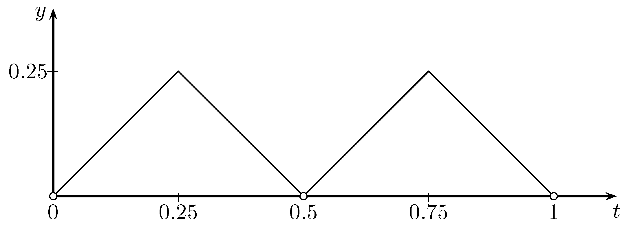
There is one more question that should be considered explicitly. What is the maximum value of k that we may access in the calling sequence evalf[m₀ + 3 + k](p)? We provide here an analysis of this possibility. We set on the intervals $(0,0.5)$ and $(0.5,1)$ the functions $f(t)$ and $g(t)$, respectively, such that

$$f(t)=\min \{t,0.5-t\}=\left\{\begin{array}{cc}t\hfill & \mathrm{as}0<t\le 0.25,\hfill \\ 0.5-t\hfill & \mathrm{as}0.25<t<0.5.\hfill \end{array}\right.$$

and

$$g(t)=\min \{1-t,t-0.5\}=\left\{\begin{array}{cc}t-0.5\hfill & \mathrm{as}0.5<t\le 0.75,\hfill \\ 1-t\hfill & \mathrm{as}0.75<t<1.\hfill \end{array}\right.$$

Then, we define

$$M(t)=\left\{\begin{array}{cc}f(t)\hfill & \mathrm{as}0<t<0.5,\hfill \\ g(t)\hfill & \mathrm{as}0.5<t<1.\hfill \end{array}\right.$$

and give its graph in Figure 1.

Now, reaching (16) or (17) at the step k can be expressed as

$$\frac{|x|}{2.4\times {10}^{m_0}}\le {10}^{k}M(t_k).$$

Because $|x|/{10}^{m_0}\le 1/{10}^{r+2}$, we can attain this when

$$\frac{1}{2.4\times {10}^{r+2}}\le {10}^{k}M(t_k).$$

(20)

Taking integral values from $0,1,\dots$, the variable k makes the value of the right side of (20) increase very fast, whereas the positive values of $M(t_k)$ slightly change when k increases. We also have the estimate $|M(t)-M(t^{\prime })|\le |t-t^{\prime }|$ for all $t,t^{\prime }\in (0,0.5)\cup (0.5,1)$. Thus, the minimum value of $m_k=m_0+k$ satisfying (16) or (17) is governed by $m_0$. In practice, since $|x|$ and r are not too large, we may always determine such a value of $m_k$.

On the other hand, if we find a sequence of rational numbers $\{q_n\}$ converging to $p=\pi /2$ and a strictly increasing sequence of natural numbers $\{m_n\}$ such that

$$|p-q_n|<\frac{1}{{10}^{m_n}}<\frac{1}{|x|{10}^{r+2}},n=0,1,\dots ,$$

we can determine $k_0$, following the above steps without using the command evalf (or other equivalent commands).

According to the choice of $k_0$, we always have $|x-k_0{p}^{\prime }|\le p^{\prime }/2<0.8$. Now, we check that

$$|x-k_{0}p|<0.8$$

(21)

for all choices of $k_0$. In the cases of $x/p^{\prime }-\lfloor x/p^{\prime }\rfloor <1/2$ or $x/p^{\prime }-\lfloor x/p^{\prime }\rfloor >1/2$, we also have $x/p-\lfloor x/p\rfloor <1/2$ or $x/p-\lfloor x/p\rfloor >1/2$ and easily check that $|x/p-k_0|<1/2$ or $|x-k_{0}p|<p/2<0.8$. In the case $x/p^{\prime }-\lfloor x/p^{\prime }\rfloor =1/2$, since (6), (9) and (10) are all satisfied, we have $\lfloor x/p^{\prime }\rfloor =\lfloor x/p\rfloor$ and need to check (21) directly. Indeed, we can write

$$0<\frac{x}{p}-k_0=\frac{x}{p}-⌊\frac{x}{p^{\prime }}⌋=\frac{x}{p^{\prime }}\pm \frac{\sigma |x|}{p{p}^{\prime }}-⌊\frac{x}{p^{\prime }}⌋=\frac{1}{2}\pm \frac{\sigma |x|}{p{p}^{\prime }},$$

hence

$$x-k_{0}p<\frac{p}{2}+\frac{\sigma |x|}{p^{\prime }}<\frac{p}{2}+\frac{1}{p^{\prime }{10}^{r+2}}<\frac{3.1416}{4}+\frac{1}{1.5\times {10}^3}<0.79+0.0067<0.8.$$

We formalize the above discussion by the following lemma.

Lemma 1.

For every rational number x, there exists an integer $k_0$ and a rational approximation $p^{\prime }$ of $p=\pi /2$ such that $\lfloor x/p^{\prime }\rfloor =\lfloor x/p\rfloor$, and $k_0=\lfloor x/p^{\prime }\rfloor$ or $k_0=\lfloor x/p^{\prime }\rfloor +1$, depending on $x/p^{\prime }-\lfloor x/p^{\prime }\rfloor \le 1/2$ or $x/p^{\prime }-\lfloor x/p^{\prime }\rfloor >1/2$, respectively. Moreover, the Taylor polynomial $P_n$ of the sine function at $x_0=k_{0}p$ can give the approximation $\sin x\approx P_n(x)$ with the accuracy up to $1/{10}^r$, where r is a given positive integer and the degree of $P_n$ is determined by(2).

In practice, since we cannot use $P_n$ from (4) or (5) to approximate the value of the sine function at x, we replace $P_n$ with $P_n^c$ instead. Such a changed polynomial can be either

$$\begin{array}{cc}\hfill P_n^c(x)& ={(-1)}^{(k_0-1)/2}\sum _{m=0}^{\lfloor n/2\rfloor }\frac{{(-1)}^m}{(2m)!}{(x-k_0{p}^{\prime })}^{2m},\mathrm{or}\hfill \end{array}$$

(22)

$$\begin{array}{cc}\hfill P_n^c(x)& ={(-1)}^{k_0/2}\sum _{m=0}^{\lfloor (n-1)/2\rfloor }\frac{{(-1)}^m}{(2m+1)!}{(x-k_0{p}^{\prime })}^{2m+1},\hfill \end{array}$$

(23)

depending on $k_0$ odd or even, respectively. Because $|x-k_{0}p|<0.8$, we derive the estimate $|\sin x-P_n(x)|\le \delta$ from (2). Now, we need to estimate ${\delta }^{\prime }=|\sin x-P_n^c(x)|$, which we shall call the practical error.

Firstly, we choose the polynomial (22) and try to make an estimate for

$${\delta }^{\prime }=|\sin x-{(-1)}^{k_1}\sum _{m=0}^{\lfloor n/2\rfloor }\frac{{(-1)}^m}{(2m)!}{(x-k_0{p}^{\prime })}^{2m}|=|\sin x-{(-1)}^{k_1}\sum _{m=0}^{\lfloor n/2\rfloor }\frac{{(-1)}^m}{(2m)!}{(x-k_{0}p\pm k_0\sigma )}^{2m}|$$

or

$${\delta }^{\prime }=|\sin x-{(-1)}^{k_1}\sum _{m=0}^{\lfloor n/2\rfloor }\frac{{(-1)}^m}{(2m)!}\sum _{k=0}^{2m}\left(\genfrac{}{}{0pt}{}{2m}{k}\right){(x-k_{0}p)}^{2m-k}{(\pm k_0\sigma )}^k|.$$

(24)

Since

$$\sum _{k=0}^{2m}\left(\genfrac{}{}{0pt}{}{2m}{k}\right){(x-k_{0}p)}^{2m-k}{(\pm k_0\sigma )}^k={(x-k_{0}p)}^{2m}+\sum _{k=1}^{2m}\frac{(2m)!}{k!(2m-k)!}{(x-k_{0}p)}^{2m-k}{(\pm k_0\sigma )}^k,$$

(24) can be written as

$${\delta }^{\prime }=|\sin x-{(-1)}^{k_1}\sum _{m=0}^{\lfloor n/2\rfloor }\frac{{(-1)}^m}{(2m)!}{(x-k_{0}p)}^{2m}-{(-1)}^{k_1}\sum _{m=1}^{\lfloor n/2\rfloor }{(-1)}^m\sum _{k=1}^{2m}\frac{{(x-k_{0}p)}^{2m-k}{(\pm k_0\sigma )}^k}{k!(2m-k)!}|,$$

hence we obtain the estimate

$${\delta }^{\prime }\le \delta +\left|\sum _{m=1}^{\lfloor n/2\rfloor }{(-1)}^m\sum _{k=1}^{2m}\frac{{(x-k_{0}p)}^{2m-k}{(\pm k_0\sigma )}^k}{k!(2m-k)!}\right|.$$

(25)

Letting $|k_0|\sigma =\beta$, from (21) and (25), we derive

$${\delta }^{\prime }\le \delta +\sum _{m=1}^{\lfloor n/2\rfloor }{(0.8)}^{2m}\sum _{k=1}^{2m}{\left(\frac{\beta }{0.8}\right)}^k\frac{1}{k!(2m-k)!}.$$

(26)

To estimate the sum in (26), we will use inequalities related to factorial numbers, so we need some properties of the generalized factorial function, the Gamma function:

$$\Gamma (z)={\int }_0^{\infty }{e}^{-t}{t}^{z-1}dt.$$

$\Gamma (z)$ has been proven to be a log-convex function on the interval $(0,\infty )$; thus, for $y,z\in (0,\infty )$ we have

$$\Gamma \left(\frac{y+z}{2}\right)\le \sqrt{\Gamma (y)\Gamma (z)}$$

(27)

(see [12] Section 2). In addition, for a non-negative integer n, we have $\Gamma (n+1)=n!$, and for $y=k+1$, $z=2m-k+1$ with integers $m,k$ satisfying $1\le k\le 2m$, we derive the following inequality from (27)

$$m!\le \sqrt{k!(2m-k)!}\mathrm{or}\frac{1}{k!(2m-k)!}\le \frac{1}{{(m!)}^2}.$$

(28)

From (26) and (28), we can write

$${\delta }^{\prime }\le \delta +\sum _{m=1}^{\lfloor n/2\rfloor }\frac{{(0.8)}^{2m}}{{(m!)}^2}\sum _{k=1}^{2m}{\left(\frac{\beta }{0.8}\right)}^k<\delta +\frac{\beta }{0.8-\beta }\sum _{m=1}^{\lfloor n/2\rfloor }\frac{{(0.8)}^{2m}}{{(m!)}^2},$$

(29)

due to $1-{(\beta /0.8)}^{2m}<1$.

To obtain the desired estimate of ${\delta }^{\prime }$, we use an approximate value of the Modified Bessel function of the First kind

$$I_{\nu }(x)=\sum _{m=0}^{\infty }\frac{{(x/2)}^{2m+\nu }}{m!\Gamma (m+1+\nu )},$$

which is

$$I_0(1.6)=\sum _{m=0}^{\infty }\frac{{(0.8)}^{2m}}{{(m!)}^2}<1.75,$$

according to the approximation formula in ([13] Section 3). Moreover, we have the estimate

$$\beta <\frac{2}{{10}^{r+2}}$$

that we now check only for $x>0.8$. Indeed, if $k_0=\lfloor x/p^{\prime }\rfloor$, then $k_0\le x/p^{\prime }$, hence $|k_0/x|\le 1/p^{\prime }$; if $k_0=\lfloor x/p^{\prime }\rfloor +1$, we have $k_0-1\le x/p^{\prime }$ or $|k_0/x|=k_0/x\le 1/p^{\prime }+1/x<1/p^{\prime }+1/0.8<2$. These estimates for $|k_0/x|$ lead to

$$\beta =|k_0|\sigma \le \frac{|k_0|}{|x|{10}^{r+2}}<\frac{2}{{10}^{r+2}}.$$

Finally, from (28), we derive

$${\delta }^{\prime }<\delta \delta +\frac{\beta }{0.8-\beta }(1.75-1)<\frac{40}{40\times {10}^r-1}+\frac{0.75}{40\times {10}^r-1}=\frac{40.75}{40\times {10}^r-1}<\frac{1.1}{{10}^r}.$$

Similarly, if the polynomial (23) has been chosen, we are led to the estimate

$${\delta }^{\prime }\le \delta +\sum _{m=1}^{\lfloor (n-1)/2\rfloor }{(0.8)}^{2m+1}\sum _{k=1}^{2m+1}{\left(\frac{\beta }{0.8}\right)}^k\frac{1}{k!(2m+1-k)!}.$$

(30)

In this case, applying (27), we obtain the inequality

$$\frac{1}{k!(2m+1-k)!}\le \frac{1}{{\left[\Gamma (m+1+1/2)\right]}^2}.$$

(31)

To estimate the right-hand side of (31), we use an appropriate inequality of Lazarević and Lupaş in ([12] p. 95–96), stated in the form of

$${\left(z-\frac{1-\mu }{2}\right)}^{\mu }\le \frac{\Gamma (z+\mu )}{\Gamma (z)},$$

(32)

where $z>(1-\mu )/2$ and $\mu \in [0,1]$. Applying (32) for $z=m+1$ ($m=0,1,\dots$) and $\mu =1/2$, we easily obtain the inequality

$$\frac{1}{{\left[\Gamma (m+1+1/2)\right]}^2}\le \frac{1}{{(m!)}^2(m+3/4)}\le \frac{4}{7{(m!)}^2},m=1,2,\dots .$$

(33)

Combining (30), (31) and (33), we finally get the desired estimate

$${\delta }^{\prime }<\delta +\frac{\beta }{0.8-\beta }\times \frac{4\times (0.8)(1.75-1)}{7}<\frac{40}{40\times {10}^r-1}+\frac{0.35}{40\times {10}^r-1}<\frac{1.1}{{10}^r}.$$

Thus, both of approximate polynomials (22) and (23) satisfy the same inequality for the practical error; that is

$$|\sin x-P_n^c(x)|<\frac{1.1}{{10}^r}.$$

Finally, for a real number x and its rational approximation $x^{\prime }$, we have the following estimation

$$|\sin x-P_n^c(x^{\prime })|\le |\sin x-\sin x^{\prime }|+|\sin x^{\prime }-P_n^c(x^{\prime })|<|x-x^{\prime }|+\frac{1.1}{{10}^r},$$

where $P_n^c$ is obtained from $P_n$, as indicated in Lemma 1, but for $x^{\prime }$ instead. If r is replaced with $r+1$ in (2) and (6), and $|x-x^{\prime }|<1/{10}^{r+1}$, then $|\sin x-P_n^c(x^{\prime })|<1/{10}^r$.

To sum up, we state our main result in this section by the following theorem.

Theorem 1.

Let x be a real number and $x^{\prime }$ be a rational approximation of x such that $|x-x^{\prime }|<1/{10}^{r+1}$, where r is a given positive integer. Then, from Lemma1 applied to $x^{\prime }$, there exists a polynomial $P_n^c$ having the form of (22) or (23) that gives the approximation $|\sin x-P_n^c(x^{\prime })|<1/{10}^r$.

4. Algorithm for Pointwise Polynomial Approximation

Given a rational number x and an integer $h\ge 2$, we will construct an algorithm to evaluate the approximate value a of $\sin x$ so that ${\delta }^{\prime }=|\sin x-a|$ is less than an arbitrarily small tolerance, and to display the result in the correct number h of significant digits. The first task can be completed by the steps in Algorithm 1, following the steps as indicated in Section 3, above Lemma 1. This algorithm can be converted into a MAPLE procedure called ApproxSine that takes the two arguments x and r. The output of ApproxSine(x,r) is a with ${\delta }^{\prime }<1/{10}^r$, $r\ge 1$. This estimation for ${\delta }^{\prime }$ is obtained when r is replaced with $r+1$ in (2) and (6). Before completing the second task, we note that the accuracy up to the r-th decimal digit after decimal point is in general quite different from r significant digits. For instance, if $a=0.123437$ and $b=0.123415$, then $|a-b|<1/{10}^4$ and evalf[4](a) = evalf[4](b), but, if $a=0.0024217$ and $b=0.002421$, then evalf[6](a) ≠ evalf[6](b), whereas $|a-b|<1/{10}^6$. Therefore, we should first count how many zero consecutive digits there are right after decimal point contained in the number a = ApproxSine(x,r), and assume that the number of such digits is k, which is $a=0.\underset{k\mathrm{digits}}{\underbrace{00\cdots 0}}xy\cdots z$ ($x\ne 0$). In fact, the number k can be determined easily, for instance, by a simple while-do loop in MAPLE as follows:

> a:=ApproxSine(x,h):

> k:=0:

> while (abs(a)*10^k-1<0) do

> k:=k+1:

> end do:

Then, the second task can be completed by displaying the output of ApproxSine(x,k + h + 1) in h significant digits, which is the calling evalf[h](ApproxSine(x,k + h + 1)). Now, we can make another MAPLE procedure named Sine to perform the second task when using ApproxSine as its local variable. The calling sequence Sine(x,h) returns an approximate value a of $\sin x$ such that the correct number of significant digits of a is equal to h. In the following, we present Algorithm 1 as a pseudo-code algorithm as

Algorithm 1

Input:x (rational number), r (positive integer)

Output:$a\approx \sin x$ with $|\sin x-a|<1/{10}^r$

Similarly, for approximating values of the cosine function, we use the Taylor polynomial of $g(y)=\cos y$:

$$Q_n(y)=\sum _{m=0}^n\frac{g^{(m)}(x_0)}{m!}{(y-x_0)}^m,$$

where $x_0=k_{0}p$ and

$$g^{(m)}(k_{0}p)=\left\{\begin{array}{cc}0,& m+k_0=2k+1,\hfill \\ {(-1)}^k,& m+k_0=2k(k\in \mathbb{Z}).\hfill \end{array}\right.$$

The integer $k_0$ is determined by the same way as the one in the previous sections and the index k satisfies

$$\frac{k_0}{2}\le k\le \frac{k_0+n}{2},$$

due to $0\le m\le n$. Hence, depending on $k_0$ even or odd, $g(x)=\cos x$ is approximated by

$$Q_n(x)={(-1)}^{k_0/2}\sum _{m=0}^{\lfloor n/2\rfloor }\frac{{(-1)}^m}{(2m)!}{(x-k_{0}p)}^{2m}$$

or

$$Q_n(x)={(-1)}^{(k_0+1)/2}\sum _{m=0}^{\lfloor (n-1)/2\rfloor }\frac{{(-1)}^m}{(2m+1)!}{(x-k_{0}p)}^{2m+1},$$

respectively. Then, we have a similar algorithm to evaluate approximate values of $\cos x$ and a corresponding MAPLE procedure Cosine taking the same arguments x and h. In the body of Cosine, ApproxSine becomes its local variable ApproxCosine when the variable a in ApproxSine (as a in Algorithm 1) is assigned to these corresponding values of $Q_n$. Cosine also returns approximate values of the cosine function in a given correct number of significant digits. In practice, $Q_n(x)$ becomes $Q_n^c(x)$ when $p^{\prime }$ takes the position of p, and again we can check the estimate $|\cos x-Q_n^c(x)|<1.1/{10}^r$. As a convention, we will present all algorithms afterwards in a pseudo–code form and use corresponding MAPLE procedures with names to make calculations. Now, we implement our algorithms with some values of x and h, and the results of the calling sequences Sine(x,r) and Cosine(x,r) are given in

Table 1. Some results from using the procedures Sine and Cosine.

Calling Sequences	Results
Sine(123,25)	$-0.4599034906895912512924357$
Sine(−1500.024,35)	$0.99626189049405202369399458834570209$
Cosine(578.99,40)	$0.5922469285742675816988406427238119209980$
Cosine(3.1415926535,45)	$-0.999999999999999999995968587163195430469041636$

.

5. Algorithm for Piecewise Polynomial Approximation

We recall here what is needed for initial settings to the piecewise approximation process. For a given number $\alpha$, we find an integer $k_0$ such that the Taylor polynomial $P_n$ at $k_{0}p$, $p=\pi /2$, can be used to approximate $\sin \alpha$ with the accuracy of $1/{10}^r$, where r is a given positive integer. Because we only get rational approximate values of p, we have found a way (as presented in previous sections) to determine such a value $p^{\prime }$, remaining the approximation $\sin \alpha \approx P_n^c(\alpha )$ with the accuracy of $1/{10}^r$, where $P_n^c$ is obtained from $P_n$ by replacing p with $p^{\prime }$. In addition, we have proved that $|\alpha -k_{0}p|<0.8$, or likewise $|\alpha -k_0{p}^{\prime }|<0.8$ and

$$\sigma =|p-p^{\prime }|<\frac{1}{\gamma {10}^{r+3}},$$

(34)

where $|k_0|\le \gamma$. In fact, more exactly, we have $|\alpha -k_0{p}^{\prime }|<0.788$ and $0.8-p^{\prime }/2>0.012$ for such a chosen $p^{\prime }$. Moreover, for every $x\in [k_0{p}^{\prime }-p^{\prime }/2,k_0{p}^{\prime }+p^{\prime }/2]$, we can use $P_n^c$ to approximate $\sin x$ because of $|x-k_{0}p|<0.8$ (note that $|x-k_0{p}^{\prime }|\le p^{\prime }/2<0.8$). Indeed, we have the estimate

$$|x-k_{0}p|=|x-k_0{p}^{\prime }+k_0{p}^{\prime }-k_{0}p|\le \frac{p^{\prime }}{2}+|k_0||p-p^{\prime }|<\frac{p^{\prime }}{2}+|k_0|\sigma ,$$

and get the desired inequality when $|k_0|\sigma <0.8-p^{\prime }/2$ or more strictly, $|k_0|\sigma <0.012$. However, this is obviously satisfied because

$$\frac{|k_0|}{\gamma {10}^{r+3}}\le \frac{1}{{10}^{r+3}}<0.012.$$

Therefore, we have the approximation

$$\sin \approx P_n^c\mathrm{on}[k_0{p}^{\prime }-p^{\prime }/2,k_0{p}^{\prime }+p^{\prime }/2],$$

(35)

with the accuracy of $1/{10}^r$ if we replace r with $r+1$. This extension of our pointwise approximating result can be a starting point to construct a piecewise function F that approximates the sine function on an interval $[a,b]$.

From most parts of Algorithm 1 (only without Step 2), we can derive a simpler algorithm that results in three objects k, $p^{\prime }$ and $P_n^c$ (respectively, $k_0$, p and a in Algorithm 1) from an input number $\alpha$. For convenience, we will use the name FindPoint of a MAPLE procedure performing such an algorithm with one real argument, so its usage can be given in one of the forms: FindPoint(α) = [k,$P^{\prime }$,$P_n^c$], FindPoint(α)[1] = k, FindPoint(α)[2] = $P^{\prime }$ and FindPoint(α)[1] = $P_n^c$.

Because the sine function is odd, we only need to find the function F on $[a,b]$ with $a\ge 0$. In the cases of $0\le a<b\le 0.8$ and $0\le a<0.8<b$, we may set $F=F_0$ on $[a,b]$ and $F=F_0$ on $[a,0.8]$, respectively, where

$$F_0(x)=\sum _{m=0}^{\lfloor (n-1)/2\rfloor }\frac{{(-1)}^m}{(2m+1)!}{x}^{2m+1}$$

and n is determined by Algorithm 1. Therefore, it is sufficient to construct a piecewise approximate function F on $[a,b]$ when $0.8\le a<b$.

On the other hand, from the choice of $\sigma =|p-p^{\prime }|<1/(|x|{10}^{r+3})$ in Algorithm 1 to approximate $\sin x$, we now change it to

$$\sigma =|p-p^{\prime }|<\frac{1}{(b+3.2){10}^{r+3}}\mathrm{for}\mathrm{all}x\in [a,b].$$

(36)

This choice is to guarantee the precision for our later construction of F. Moreover, it is easy to check that if $\alpha ,\beta \in [a,b]$ are numbers such that

$$\mathtt{FindPoint}\mathtt{(}\alpha \mathtt{)}\mathtt{[}\mathtt{1}\mathtt{]}=\mathtt{FindPoint}\mathtt{(}\beta \mathtt{)}\mathtt{[}\mathtt{1}\mathtt{]}=k$$

$\mathrm{with}$ $P^{\prime }$ = FindPoint($\alpha$)[2], $P^{″}$ = FindPoint($\beta$)[2] then we have |α − ${\mathrm{kP}}^{″}$| < 0.8 and |β − ${\mathrm{kP}}^{\prime }$| < 0.8.

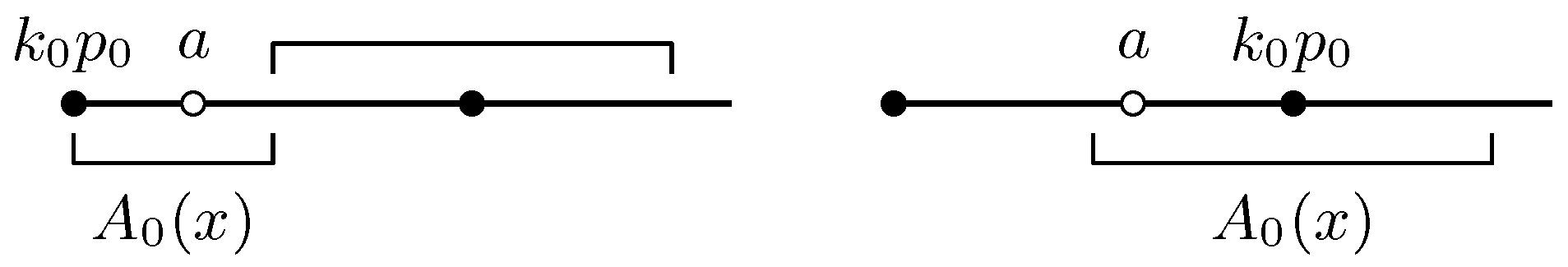
Firstly, we put

$$\begin{array}{cc}\hfill n_0& =\mathtt{FindPoint}(b\mathtt{)}\mathtt{[}\mathtt{1}\mathtt{]},\hfill \\ \hfill q_0& =\mathtt{FindPoint}\mathtt{(}b\mathtt{)}\mathtt{[}\mathtt{2}\mathtt{]}\mathrm{and}\hfill \\ \hfill B_0& =\mathtt{FindPoint}\mathtt{(}b\mathtt{)}\mathtt{[}\mathtt{3}\mathtt{]},\hfill \end{array}$$

and similarly,

$$\begin{array}{cc}\hfill k_0& =\mathtt{FindPoint}\mathtt{(}a\mathtt{)}\mathtt{[}\mathtt{1}\mathtt{]},\hfill \\ \hfill p_0& =\mathtt{FindPoint}\mathtt{(}a\mathtt{)}\mathtt{[}\mathtt{2}\mathtt{]}\mathrm{and}\hfill \\ \hfill A_0& =\mathtt{FindPoint}\mathtt{(}a\mathtt{)}\mathtt{[}\mathtt{3}\mathtt{]}.\hfill \end{array}$$

The cases of $k_0=\lfloor a/p_0\rfloor$ and $k_0=\lfloor a/p_0\rfloor +1$ are illustrated in Figure 2.

Now, we consider the case $k_0=n_0$ (or even $k_0=n_0+1$); then, we choose $F=A_0$ on $[a,b]$ because $|b-k_0{p}_0|<0.8$ as shown above for $\alpha ,\beta$. Next, we consider the case when $k_0<n_0$. We extend the approximation process to determine the next integer by setting $k_1=\mathtt{FindPoint}($(k₀ +1 )p₀$\mathtt{)}\mathtt{[}\mathtt{1}\mathtt{]}$, and also $p_1=\mathtt{FindPoint}($(k₀ + 1)p₀$\mathtt{)}\mathtt{[}\mathtt{2}\mathtt{]}$, $A_1=\mathtt{FindPoint}($(k₀ +1 )p₀$\mathtt{)}\mathtt{[}\mathtt{3}\mathtt{]}$. Because $|(k_0+1)p_0-k_1{p}_1|<0.8$, by the choice of $k_1$, we must have $k_1=k_0+1$. 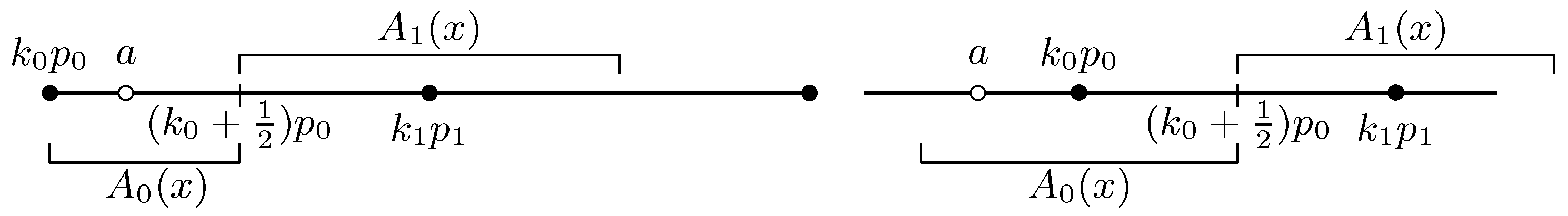Note that, from (36), we also have $|(k_0+\frac{1}{2})p_0-k_1{p}_1|<0.8$. If $k_1=n_0$, we then have cases that are illustrated in Figure 3. It is obvious that we can set $F=A_0$ on $[a,(k_0+\frac{1}{2})p_0]$, regardless of $k_0=\lfloor a/p_0\rfloor$ or $k_0=\lfloor a/p_0\rfloor +1$. However, we will take different settings on the other intervals, depending on where b is from $(k_0+1)p_0$. These settings can be given in the following:

$$\begin{array}{cc}\hfill b\le (k_0+\frac{1}{2})p_0& :F=A_0\mathrm{on}[a,b].\hfill \\ \hfill (k_0+\frac{1}{2})p_0<b\le (k_0+1)p_0& :F=\left\{\begin{array}{cc}{A}_0\hfill & \mathrm{on}[a,(k_0+\frac{1}{2})p_0),\hfill \\ A_1\hfill & \mathrm{on}[(k_0+\frac{1}{2})p_0,b].\hfill \end{array}\right.\hfill \\ \hfill (k_0+1)p_0<b& :F=\left\{\begin{array}{cc}{A}_0\hfill & \mathrm{on}[a,(k_0+\frac{1}{2})p_0),\hfill \\ A_1\hfill & \mathrm{on}[(k_0+\frac{1}{2})p_0,(k_0+1)p_0),\hfill \\ B_0\hfill & \mathrm{on}[(k_0+1)p_0,b].\hfill \end{array}\right.\hfill \end{array}$$

(37)

If $k_1<n_0$, we continue to put

$$\begin{array}{cc}\hfill k_2& =\mathtt{FindPoint}\mathtt{(}(k_{\mathtt{1}}+\mathtt{1})p_1\mathtt{)}\mathtt{[}\mathtt{1}\mathtt{]},\hfill \\ \hfill p_2& =\mathtt{FindPoint}\mathtt{(}(k_{\mathtt{1}}+\mathtt{1})p_1\mathtt{)}\mathtt{[}\mathtt{2}\mathtt{]},\hfill \\ \hfill A_2& =\mathtt{FindPoint}\mathtt{(}(k_{\mathtt{1}}+\mathtt{1})p_1\mathtt{)}\mathtt{[}\mathtt{3}\mathtt{]}.\hfill \end{array}$$

In the case of $k_2=n_0$, we have the following choice for F according to the different positions of b from $(k_1+1)p_1$:

$$\begin{array}{cc}\hfill b\le (k_1+\frac{1}{2})p_1& :F=\left\{\begin{array}{cc}{A}_0\hfill & \mathrm{on}[a,(k_0+\frac{1}{2})p_0),\hfill \\ A_1\hfill & \mathrm{on}[(k_0+\frac{1}{2})p_0,b].\hfill \end{array}\right.\hfill \\ \hfill (k_1+\frac{1}{2})p_1<b\le (k_1+1)p_1& :F=\left\{\begin{array}{cc}{A}_0\hfill & \mathrm{on}[a,(k_0+\frac{1}{2})p_0),\hfill \\ A_1\hfill & \mathrm{on}[(k_0+\frac{1}{2})p_0,(k_1+\frac{1}{2})p_1),\hfill \\ A_2\hfill & \mathrm{on}[(k_1+\frac{1}{2})p_1,b].\hfill \end{array}\right.\hfill \\ \hfill (k_1+1)p_1<b& :F=\left\{\begin{array}{cc}{A}_0\hfill & \mathrm{on}[a,(k_0+\frac{1}{2})p_0),\hfill \\ A_1\hfill & \mathrm{on}[(k_0+\frac{1}{2})p_0,(k_1+\frac{1}{2})p_1),\hfill \\ A_2\hfill & \mathrm{on}[(k_1+\frac{1}{2})p_1,(k_1+1)p_1),\hfill \\ B_0\hfill & \mathrm{on}[(k_1+1)p_1,b].\hfill \end{array}\right.\hfill \end{array}$$

(38)

Finally, continuing the above process, we obtain a finite sequence $k_0$, $k_1$, …, $k_n$ such that $k_i=k_{i-1}+1=\mathtt{FindPoint}\mathtt{(}$(k_i−1 + 1)p_i−1$\mathtt{)}\mathtt{[}\mathtt{1}\mathtt{]}$, $i=1,\dots ,n-1$, and $k_n=n_0$. Then, we also gain two sequences $p_i=\mathtt{FindPoint}\mathtt{(}$(k_i−1 + 1)p_i−1$\mathtt{)}\mathtt{[}\mathtt{2}\mathtt{]}$ and $A_i=\mathtt{FindPoint}\mathtt{(}$(k_i−1 + 1)p_i−1$\mathtt{)}\mathtt{[}\mathtt{3}\mathtt{]}$, $i=1,\dots ,n$. Before giving our settings for this general case, let us consider ending points of the approximate intervals by taking two consecutive nodes $k_i{p}_i$, $k_{i+1}{p}_{i+1}$. If we let $x_i=k_i{p}_i+p_i/2$, then we have $|x_i-k_{i+1}{p}_{i+1}|=k_i(p_{i+1}-p_i)+p_{i+1}-p_i/2$, so that

$$|x_i-k_{i+1}{p}_{i+1}|<0.8\mathrm{if}\mathrm{and}\mathrm{only}\mathrm{if}(k_i+1)(p_{i+1}-p_i)<0.8-p_i/2.$$

(39)

To show the assertion of (39), we refer to (36) again and take the same arguments as above. The inequality (39) explains why we can choose F on $[a,b]$ to guarantee the accuracy of $1/{10}^r$.

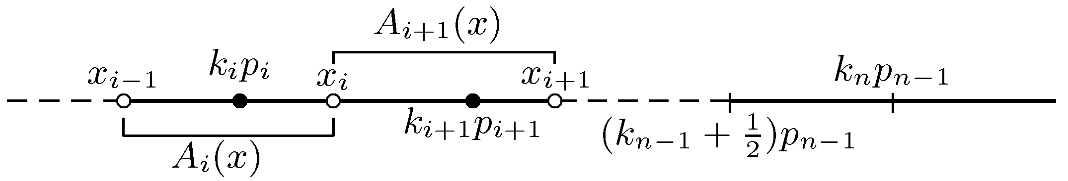
In short, by the setting (36), when $k_n=n_0$ with $n\ge 3$ (see Figure 4), we have constructed the piecewise function F that approximates the sine function on $[a,b]$ ($0.8\le a<b$) with the accuracy of $1/{10}^r$. After getting the finite sequences ${\{k_i\}}_{i=0}^n$, ${\{p_i\}}_{i=0}^n$, ${\{A_i\}}_{i=0}^n$ and the function $B_0$ defined as above, we choose F as follows:

• If $b\le (k_{n-1}+\frac{1}{2})p_{n-1}$:

  $$F=\left\{\begin{array}{cc}{A}_0\hfill & \mathrm{on}[a,(k_0+\frac{1}{2})p_0),\hfill \\ A_i\hfill & \mathrm{on}[(k_{i-1}+\frac{1}{2})p_{i-1},(k_i+\frac{1}{2})p_i),i=1,\dots ,n-2,\hfill \\ A_{n-1}\hfill & \mathrm{on}[(k_{n-2}+\frac{1}{2})p_{n-2},b].\hfill \end{array}\right.$$

  (40)
• If $(k_{n-1}+\frac{1}{2})p_{n-1}<b\le k_n{p}_{n-1}$:

  $$F=\left\{\begin{array}{cc}{A}_0\hfill & \mathrm{on}[a,(k_0+\frac{1}{2})p_0),\hfill \\ A_i\hfill & \mathrm{on}[(k_{i-1}+\frac{1}{2})p_{i-1},(k_i+\frac{1}{2})p_i),i=1,\dots ,n-1,\hfill \\ A_n\hfill & \mathrm{on}[(k_{n-1}+\frac{1}{2})p_{n-1},b].\hfill \end{array}\right.$$

  (41)
• If $k_n{p}_{n-1}<b$:

  $$F=\left\{\begin{array}{cc}{A}_0\hfill & \mathrm{on}[a,(k_0+\frac{1}{2})p_0),\hfill \\ A_i\hfill & \mathrm{on}[(k_{i-1}+\frac{1}{2})p_{i-1},(k_i+\frac{1}{2})p_i),i=1,\dots ,n-1,\hfill \\ A_n\hfill & \mathrm{on}[(k_{n-1}+\frac{1}{2})p_{n-1},k_n{p}_{n-1}),\hfill \\ B_0\hfill & \mathrm{on}[k_n{p}_{n-1},b].\hfill \end{array}\right.$$

  (42)

Although steps for construction of F have been presented, we give here an abbreviated algorithm, Algorithm 2, to specifically determine this function.

In Algorithm 2, the approximate Taylor polynomials $A_i$ are derived from Algorithm 1 and given here as

$$A_i(x)={(-1)}^{(k_i-1)/2}\sum _{m=0}^{\lfloor n/2\rfloor }\frac{{(-1)}^m}{(2m)!}{(x-k_i{p}_i)}^{2m},$$

or

$${(-1)}^{k_i/2}\sum _{m=0}^{\lfloor (n-1)/2\rfloor }\frac{{(-1)}^m}{(2m+1)!}{(x-k_i{p}_i)}^{2m+1},i=0,\dots ,n,$$

depending on $k_i$ odd or even. The polynomial $B_0$ takes a similar expression, where $k_i{p}_i$ is replaced with $n_0{q}_0$.

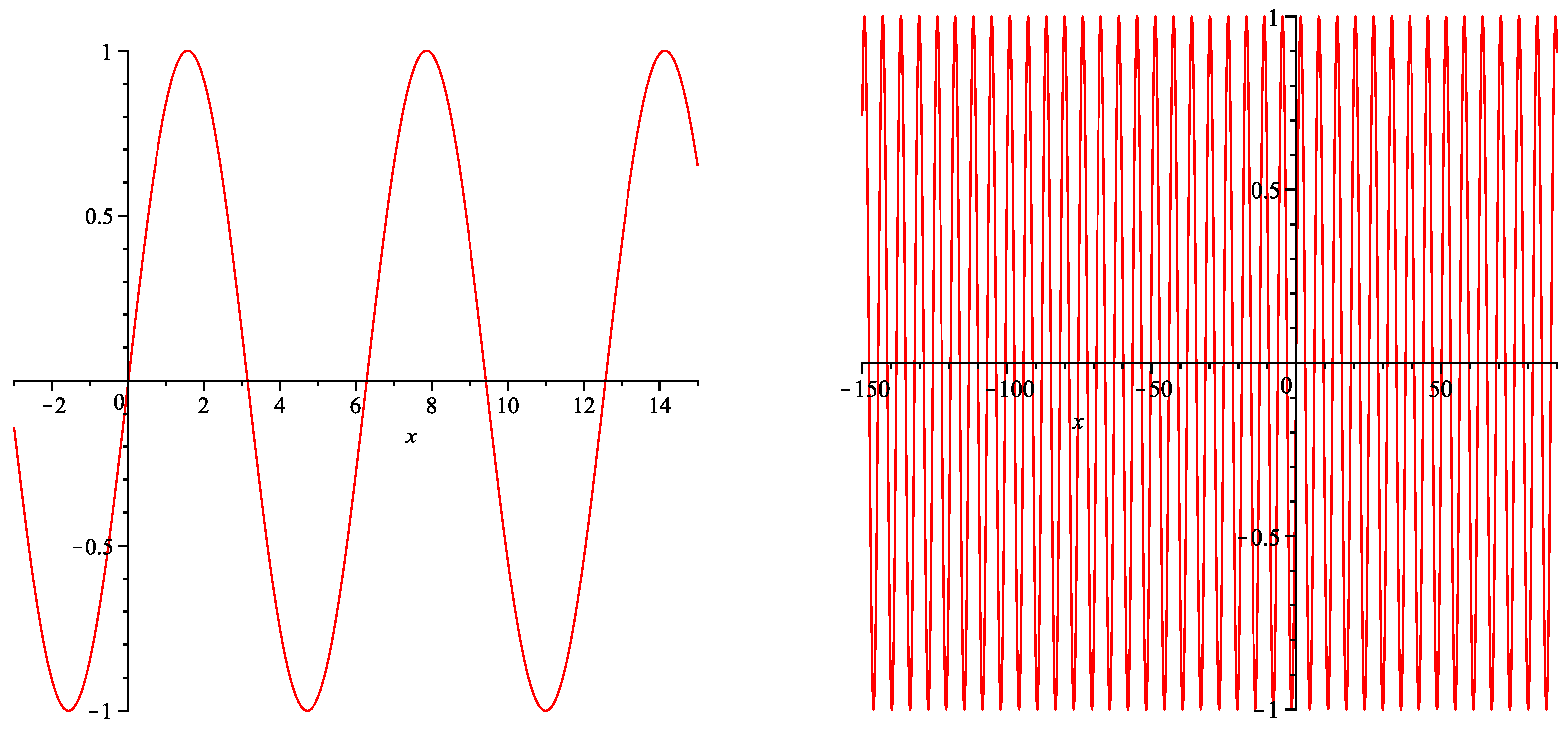
In Figure 5, the graphs of F on intervals $[a,b]$ with different values of r are depicted by a MAPLE procedure corresponding to Algorithm 2.

Algorithm 2

Input:FindPoint (the MAPLE procedure, mentioned above); $a,b$ (real numbers); r (positive integer)

Output:$F(x)$ on $[a,b]$ with $\parallel \sin -F\parallel =\sup \{|\sin x-F(x)|:x\in [a,b]\}<1/{10}^r$

To obtain a similar algorithm to approximate the cosine function, we just replace the functions $A_i$ with

$$Q_i(x)={(-1)}^{k_i/2}\sum _{m=0}^{\lfloor n/2\rfloor }\frac{{(-1)}^m}{(2m)!}{(x-k_i{p}_i)}^{2m}$$

or

$$Q_i(x)={(-1)}^{(k_i+1)/2}\sum _{m=0}^{\lfloor (n-1)/2\rfloor }\frac{{(-1)}^m}{(2m+1)!}{(x-k_i{p}_i)}^{2m+1},i=0,\dots ,n,$$

depending on $k_i$ even or odd, and $B_0$ with

$$P_0(x)=\sum _{m=0}^{\lfloor n/2\rfloor }\frac{{(-1)}^m}{(2m)!}{x}^{2m}.$$

Note that the cosine function is even, so we should regulate appropriately the function F in Algorithm 2.

6. An Application of Numerical Integration

Suppose $\sin x$ is approximated by a polynomial $P(x)$ with the accuracy up to $1/{10}^r$ on an interval $[\alpha ,\beta ]$. Then, we will find an estimation of the absolute error for ${\sin }^{s}x$ and ${[P(x)]}^s$ with some natural number s. One of the possibilities to compute ${\sin }^{s}x$ via $\sin \left((n-k)x\right)$ is given in ([14] Lemma 1.3), but here we use our previously established results as follows. Firstly, we can write

$$\sin x=P(x)+\epsilon ,$$

where $|\sin x-P(x)|=|\epsilon |={\delta }^{\prime }<1/{10}^r$ and we also have $|P(x)|<1+(1/{10}^r)=:d$ for all $x\in [\alpha ,\beta ]$. Hence, we have that

$${\sin }^{s}x={\left[P(x)+\epsilon \right]}^s=\sum _{k=0}^s\left(\genfrac{}{}{0pt}{}{s}{k}\right){[P(x)]}^{s-k}{\epsilon }^k={[P(x)]}^s+\sum _{k=1}^s\left(\genfrac{}{}{0pt}{}{s}{k}\right){[P(x)]}^{s-k}{\epsilon }^k.$$

From this relation, we easily derive the estimate

$$|{\sin }^{s}x-{[P(x)]}^s|\le d^s\sum _{k=1}^s\left(\genfrac{}{}{0pt}{}{s}{k}\right){({\delta }^{\prime }/d)}^k.$$

(43)

Now, applying (28), we obtain

$$\left(\genfrac{}{}{0pt}{}{s}{k}\right)=\frac{s!}{k!(s-k)!}\le \frac{\Gamma (s+1)}{{\left[\Gamma (1+s/2)\right]}^2},$$

(44)

and relying on the inequality ([15] p. 93), we imply

$$\Gamma \left(\frac{s}{2}+\frac{1}{2}\right)\le \sqrt{\frac{s}{2}}\Gamma \left(\frac{s}{2}\right).$$

(45)

Using (44), (45) and the formulas in [15], such as

$$\Gamma (z+1)=z\Gamma (z),2^{z-1}\Gamma \left(\frac{z}{2}\right)\Gamma \left(\frac{z}{2}+\frac{1}{2}\right)=\sqrt{\pi }\Gamma (z),$$

we attain the estimate

$$\frac{\Gamma (s+1)}{{\left[\Gamma (1+s/2)\right]}^2}=\frac{s\Gamma (s)}{{\left({\displaystyle \frac{s}{2}}\right)}^2{\left[\Gamma \left({\displaystyle \frac{s}{2}}\right)\right]}^2}=\frac{4}{s}\frac{\Gamma (s)}{{\left[\Gamma \left({\displaystyle \frac{s}{2}}\right)\right]}^2}\le \sqrt{\frac{2}{\pi }}\frac{2^s}{\sqrt{s}}.$$

(46)

Finally, from (43), (46) and the formula for the sum of a geometric progression, we derive the following estimate

$$|{\sin }^{s}x-{[P(x)]}^s|\le d^s\sqrt{\frac{2}{\pi }}\frac{2^s}{\sqrt{s}}\frac{({\delta }^{\prime }/d)}{1-({\delta }^{\prime }/d)}\left[1-{({\delta }^{\prime }/d)}^s\right]<\sqrt{\frac{2}{\pi }}\frac{{(2d)}^s}{\sqrt{s}}{\delta }^{\prime },$$

also due to $d-{\delta }^{\prime }>d-(1/{10}^r)=1$.

Thus, we have proven the result stated in the following lemma.

Lemma 2.

Assume that $f(x)=\sin x$ is approximated by the polynomial $P_n^c(x)$ on an interval $[\alpha ,\beta ]$ with the accuracy up to $1/{10}^r$, derived from the Taylor polynomial $P_n(x)$ about $kp$, $k\in \mathbb{Z}$ and $p=\pi /2$, by replacing p with its rational approximation $p^{\prime }$, as constructed in the previous sections. Then, if

$$I={\int }_{\alpha }^{\beta }{x}^t{\sin }^{s}xdx(t,s\in \mathbb{N})$$

is approximated by

$$J={\int }_{\alpha }^{\beta }{x}^t{[P_n^c(x)]}^{s}dx,$$

the error $|I-J|$ has the following upper bound

$$|I-J|\le {\int }_{\alpha }^{\beta }|{\sin }^{s}x-{[P_n^c(x)]}^s{||x|}^{t}dx\le \sqrt{\frac{2}{\pi }}\frac{{(2+2/{10}^r)}^s}{\sqrt{s}{10}^r}{\int }_{\alpha }^{\beta }{|x|}^{t}dx.$$

(47)

Because the upper bound of $|I-J|$ in (47) only depends on r, s, except the integral on the right side, we then easily imply the following theorem.

Theorem 2.

Suppose an interval $[a,b]$ can be expressed as a finite union $[a,{\alpha }_1]\cup [{\alpha }_1,{\alpha }_2]\cup \cdots \cup [{\alpha }_n,b]$ and $f(x)=\sin x$ is approximated by the polynomials $P_{m_i}^c(x)$ on the intervals $[{\alpha }_{i-1},{\alpha }_i]$, $i=1,\dots ,n+1$, with the accuracy up to $1/{10}^r$, where ${\alpha }_0=a$ and ${\alpha }_{n+1}=b$. Then, if Q is an arbitrary polynomial and

$$I={\int }_a^{b}Q(x){\sin }^{s}xdx(s\in \mathbb{N})$$

is approximated by

$$J={\int }_a^{{\alpha }_1}Q(x){[P_{m_1}^c(x)]}^{s}dx+\cdots +{\int }_{{\alpha }_n}^{b}Q(x){[P_{m_{n+1}}^c(x)]}^{s}dx=\sum _{i=1}^{n+1}{\int }_{{\alpha }_{i-1}}^{{\alpha }_i}Q(x){[P_{m_i}^c(x)]}^{s}dx,$$

the error $|I-J|$ has the following upper bound

$$|I-J|\le \sqrt{\frac{2}{\pi }}\frac{{(2+2/{10}^r)}^s}{\sqrt{s}{10}^r}\sum _{i=1}^{n+1}{\int }_{{\alpha }_{i-1}}^{{\alpha }_i}|Q(x)|dx=\sqrt{\frac{2}{\pi }}\frac{{(2+2/{10}^r)}^s}{\sqrt{s}{10}^r}{\int }_a^b|Q(x)|dx.$$

(48)

Based on Algorithm 2, we have established a procedure, say AppIntSin, to approximately compute the integral given in Theorem 2 with the desired accuracy. AppIntSin’s arguments may take input values in order as for a, b, r, s and Q, and we can even choose the value for r to get the result satisfying a given tolerance. For instance, to have the estimate $|I-J|<\epsilon$, a positive integral value for r may be chosen as to satisf

$${10}^r>0.8\frac{{(2.2)}^s}{\epsilon \sqrt{s}}{\int }_a^b|Q(x)|dx,$$

(49)

due to $\sqrt{2/\pi }<0.8$ and $2+2/{10}^r<2.2$.

Let us consider the following example. Find the approximate value of

$$I={\int }_1^{100}(2x^5+x-3){\sin }^{20}xdx$$

with the accuracy up to $\epsilon ={10}^{-30}$. We first derive $r=48$ from (49) with the settings $a=1$, $b=100$, $s=20$ and $Q(x)=2x^5+x-3$. Performing Algorithm 2 with $a=1$, $b=100$ and $r=48$, we determine $n=63$, $(k_{62}+\frac{1}{2})p_{62}=99.74556674$, $k_{63}{p}_{62}=100.5309649$ and find the appropriate case (41). Then, the calling AppIntSin($1,100,48,20,Q(x)$) gives us the desired approximation to I, first put in symbolic form as

$$\begin{array}{cc}\hfill J={\int }_a^{(k_0+\frac{1}{2})p_0}Q(x){[A_0(x)]}^{s}dx& +\sum _{i=1}^{n-1}{\int }_{(k_{i-1}+\frac{1}{2})p_{i-1}}^{(k_i+\frac{1}{2})p_i}Q(x){[A_i(x)]}^{s}dx\hfill \\ & +{\int }_{(k_{n-1}+\frac{1}{2})p_{n-1}}^{b}Q(x){[A_n(x)]}^{s}dx\hfill \end{array}$$

and then in numerical value

$$J=6.055874915602438876766631353985011986803\times {10}^{10}.$$

7. Conclusions

Motivated by the powerfulness and popular use of modern computer algebra systems in terms of its ease in programming and accessibility to the value of $\pi$ with a very high accuracy, simple and easily-implemented algorithms have been designed to approximate the trigonometric functions with an arbitrary accuracy by a means of Taylor expansion. We have provided a careful analysis of the proposed approach with numerical illustrations. Nevertheless, our initial intention is not to compare or surpass other well-developed and well-established existing algorithms in the research literature; rather, we emphasize on the simplification of our methods as a computational application of CAS for which we highlight below:

• Approximating values of the trigonometric functions by Taylor polynomials with an arbitrary accuracy, taking the form of $1/{10}^r$, $r\in \mathbb{N}$.
• Using a so-called spreading technique to switch the process of pointwise approximating to that of piecewise approximating all over an arbitrary interval.
• Performing only arithmetics on very small values of finite rational numbers.
• Only using one command of CAS to access approximate values of $\pi /2$.

Our approximation method in Algorithm 2, utilizing the achievements of computing values of Pi with more and more exact significant digits and the power of current computer algebra systems, presents the special partition of an interval $[a,b]$ with nodes $k_i{p}_i$’s, where $k_i\in \mathbb{Z}$ and $p_i$ is an approximate value of $\pi /2$. This is a great advantage for local approximation to values of the sine (or cosine) function f on each definite interval because $p_i$’s are all finite rational numbers. These nodes also play a role as adjoining centers of approximation, whereas the functional coefficients $f^{(m)}$ still take their normal values $0,\pm 1$ at $k_i\pi /2$.

Our procedure, corresponding to Algorithm 1, gives not only numerical results of great precision but also a remedy for mistakes in the use of some existing mathematical software programs when displaying wrong results with a small number n of significant digits (e.g., $n<9$). In such cases, the argument x’s to approximate $\sin x$ are commonly close to $k\pi /2$’s, $k\in \mathbb{Z}$.

In addition, Theorem 2 can be applied to look for desired estimates to the best $L^2$-approximation of the sine function in the vector space ${\mathcal{P}}_{\ell }$ of polynomials of degree at most ℓ, a subspace of $L^2(a,b)$.