Solution of Fuzzy Differential Equations Using Fuzzy Sumudu Transforms

Abstract

The uncertain nonlinear systems can be modeled with fuzzy differential equations (FDEs) and the solutions of these equations are applied to analyze many engineering problems. However, it is very difficult to obtain solutions of FDEs. In this paper, the solutions of FDEs are approximated by utilizing the fuzzy Sumudu transform (FST) method. Significant theorems are suggested in order to explain the properties of FST. The proposed method is validated with three real examples.

1. Introduction

In many physical and dynamical processes, mathematical modeling leads to the deterministic initial and boundary value problems. In practice, the boundary values may be different from crisp and displays in the form of unknown parameters [1]. The qualitative behavior of solutions of the equations is associated with the errors. If the errors are random, in this case, we have a stochastic differential equation along with the random boundary value. Moreover, if the errors are not probabilistic, the fuzzy numbers are substituted by random variables [1,2]. The fuzzy derivative, as well as fuzzy differential equations (FDE), have been discussed in [3,4]. The Peano-like theorems for FDEs, and system of FDE on R (Real line) is investigated in [5]. The first-order fuzzy initial value problem, and the fuzzy partial differential equation, have been studied in [5]. The simulation of the fuzzy system is discussed in [6,7,8,9,10,11]. The application of numerical techniques for resolving FDEs has been illustrated in [12]. The Lipschitz condition and the theorem for existence and uniqueness of the solution related to FDEs, are discussed in [13,14,15]. The fractional fuzzy Laplace transformation has been mentioned in [13].

An advanced method to solve FDEs is laid down based on the Sumudu transform. Sumudu transform along with broad applications has been utilized in the area of system engineering and applied physics. Recently, Sumudu transform is popularized in order to solve fractional local differential equations [16,17,18,19,20]. In [21], Sumudu transform is suggested in order to solve fuzzy partial differential equations. Some fundamental theorems along with some properties for Sumudu transform are mentioned in [22]. In [23] the variational iteration technique is proposed utilizing Sumudu transform for solving ordinary equations.

In this paper, we use FST to approximate the solutions of the FDEs. We extend our previous work [24] by generating more theorems for describing the properties of FST. Moreover, the comparison between our method with other numerical methods has been carried out. The FST reduces the FDE to an algebraic equation. A very important property of the FST is that it can solve the equation without resorting to a new frequency domain. By utilizing the proposed technique, the fuzzy boundary value problem can be resolved directly without determining a general solution.

This paper is organized as follows: in Section 2 some definitions which have been used in this paper are given. Section 3 demonstrates the properties of FST. In Section 4 solving FDEs by utilizing FST approach is described. Three real examples are used to demonstrate the efficiency of the proposed method in Section 5. Section 6 provides the conclusion to the paper.

2. Preliminaries

Some concepts related to the fuzzy calculations are laid down in this section [25,26].

Definition 1.

A fuzzy number B is a function of $B\in E:R\to [0,1]$, in such a manner, (1) B is normal, (there exists a${}_0\in R$ in such a manner $B(a_0)=1$); (2) B is convex, $B(\gamma a+(1-\gamma )c)\ge$ min$\{B(a),B(c)\}$, $\forall a,c\in R,\forall \gamma \in [0,1]$; (3) B is upper semi-continuous on R, i.e., $B(a)\le B(a_0)+ϵ$, $\forall a\in N(a_0),$ $\forall a_0\in R$, $\forall ϵ>0,$ $N(a_0)$ is a neighborhood; (4) The set B${}^{+}=\{a\in R,B(a)>0\}$ is compact.

Definition 2.

The r-level of the fuzzy number B is defined as follows

$${[B]}^r=\{a\in R:B(a)\ge r\}$$

(1)

where $0<r\le 1$, $B\in E.$

Definition 3.

Let $B_1,B_2\in E$ and $\xi \in R$, the operations addition, subtraction, multiplication and scalar multiplication are defined as

$${[B_1\oplus B_2]}^r={[B_1]}^r+{[B_2]}^r=[{\underline{B}}_1^r+{\underline{B}}_2^r,{\overline{B}}_1^r+{\overline{B}}_2^r]$$

(2)

$${[B_1\ominus B_2]}^r={[B_1]}^r-{[B_2]}^r=[{\underline{B}}_1^r-{\underline{B}}_2^r,{\overline{B}}_1^r-{\overline{B}}_2^r]$$

(3)

$${[B_1\odot B_2]}^r=\left(\begin{array}{c}min\{{\underline{B}}_1^r{\underline{B}}_2^r,{\underline{B}}_1^r{\overline{B}}_2^r,{\overline{B}}_1^r{\underline{B}}_2^r,{\overline{B}}_1^r{\overline{B}}_2^r\}\\ max\{{\underline{B}}_1^r{\underline{B}}_2^r,{\underline{B}}_1^r{\overline{B}}_2^r,{\overline{B}}_1^r{\underline{B}}_2^r,{\overline{B}}_1^r{\overline{B}}_2^r\}\end{array}\right)$$

(4)

$${[\xi B_1]}^r=\xi {[B_1]}^r=\left\{\begin{array}{c}(\xi {\underline{B}}_1^r,\xi {\overline{B}}_1^r),\xi \ge 0\\ (\xi {\overline{B}}_1^r,\xi {\underline{B}}_1^r),\xi \le 0\end{array}\right.$$

(5)

Definition 4.

The Hausdroff distance between two fuzzy numbers $B_1$ and $B_2$ is defined as [27,28]

$$D(B_1,B_2)=\underset{0\le r\le 1}{sup}\{max(|{\underline{B}}_1^r-{\underline{B}}_2^r|,|{\overline{B}}_1^r-{\overline{B}}_2^r|)\}$$

(6)

$D(B_1,B_2)$ has the following properties

(i) 

$D(B_1\oplus u,B_2\oplus u)=D(B_1,B_2),$ $\forall B_1,B_2,u\in E$

(ii) 

$D(\xi B_1,\xi B_2)=\mid \xi \mid D(B_1,B_2),$ $\forall \xi \in R,B_1,B_2\in E$

(iii) 

$D(B_1\oplus B_2,u\oplus v)\le D(B_1,u)+D(B_2,v),$ $\forall B_1,B_2,u,v\in E$

(iv) 

$(D,E)$ is stated as complete metric space.

Definition 5.

The function $\psi :[a_1,a_2]⟶E$ is integrable on $[a_1,a_2]$, if it satisfies in the below mentioned relation

$${\int }_{a_1}^{\infty }\psi (x)dx=({\int }_{a_1}^{\infty }\underline{\psi }(x,r)dx,{\int }_{a_1}^{\infty }\overline{\psi }(x,r)dx)$$

(7)

If $\psi (x)$ be a fuzzy value function, as well as $q(x)$ be a fuzzy Riemann integrable on $[a_1,\infty ]$ so $\psi (x)\oplus q(x)$ can be a fuzzy Riemann integrable on $[a_1,\infty ]$. Therefore,

$${\int }_{a_1}^{\infty }(\psi (x)\oplus q(x))dx={\int }_a^{\infty }\psi (x)dx\oplus {\int }_a^{\infty }q(x)dx$$

(8)

According to fuzzy concept or in the case of interval arithmetic, equation $B_1=B_2\oplus s$ is not equivalent with $s=B_1\ominus B_2=B_1\oplus (-1)B_2$ or to $B_2=B_1\ominus s=B_1\oplus (-1)s$ and this is the main reason in introducing the following Hukuhara difference (H-difference).

Definition 6.

The definition of H-difference [29,30], is proposed by $B_1{\ominus }_H{B}_2=s⟺B_1=B_2\oplus s$. If $B_1{\ominus }_H{B}_2$ prevails, its r-level is ${[B_1{\ominus }_H{B}_2]}^r=[{\underline{B}}_1^r-{\underline{B}}_2^r,{\overline{B}}_1^r-{\overline{B}}_2^r]$. Precisely, $B_1{\ominus }_H{B}_1=0$ but $B_1\ominus B_1\ne 0$.

Definition 7.

Suppose $\psi :[a_1,a_2]⟶E$ and $x_0=[a_1,a_2]$. ψ is strongly generalized differentiable at $x_0,$ if for all $k>0$ adequately minute, ${\psi }^{\prime }(x_0)\in E$ exists in such a manner that

(i) 

$\exists \psi (x_0+k){\ominus }_H\psi (x_0)$, $\psi (x_0){\ominus }_H\psi (x_0-k)$ and

$$\begin{array}{c}\underset{k\to 0^{+}}{lim}\frac{\psi (x_0+k){\ominus }_H\psi (x_0)}{k}=\underset{k\to 0^{+}}{lim}\frac{\psi (x_0){\ominus }_H\psi (x_0-k)}{k}={\psi }^{\prime }(x_0)\hfill \end{array}$$

(ii) 

$\exists \psi (x_0){\ominus }_H\psi (x_0+k)$, $\psi (x_0-k){\ominus }_H\psi (x_0)$ and

$$\begin{array}{c}\underset{k\to 0^{+}}{lim}\frac{\psi (x_0){\ominus }_H\psi (x_0+k)}{(-k)}=\underset{k\to 0^{+}}{lim}\frac{\psi (x_0-k){\ominus }_H\psi (x_0)}{(-k)}={\psi }^{\prime }(x_0),\hfill \end{array}$$

(iii) 

$\exists \psi (x_0+k){\ominus }_H\psi (x_0)$, $\psi (x_0-k){\ominus }_H\psi (x_0)$ and

$$\begin{array}{c}\underset{k\to 0^{+}}{lim}\frac{\psi (x_0+k){\ominus }_H\psi (x_0)}{k}=\underset{k\to 0^{+}}{lim}\frac{\psi (x_0-k){\ominus }_H\psi (x_0)}{(-k)}={\psi }^{\prime }(x_0)\hfill \end{array}$$

(iv) 

$\exists \psi (x_0){\ominus }_H\psi (x_0+k)$, $\psi (x_0){\ominus }_H\psi (x_0-k)$ and

$$\begin{array}{c}\underset{k\to 0^{+}}{lim}\frac{\psi (x_0){\ominus }_H\psi (x_0+k)}{(-k)}=\underset{k\to 0^{+}}{lim}\frac{\psi (x_0){\ominus }_H\psi (x_0-k)}{k}={\psi }^{\prime }(x_0)\hfill \end{array}$$

Remark 1.

It is clear that case $(i)$ is H-derivative. Furthermore, a function is (i)-differentiable only when it is H-derivative.

Remark 2.

It can be concluded from [29] that, the definition of differentiability is non contradictory [31].

Let us consider $\psi :R\to E$ where $\psi (t)$ has a parametric form as $[\psi (t,r)]=[\underline{\psi }(t,r),\overline{\psi }(t,r)]$, for all $0\le r\le 1$, thus [31]

(i)

If $\psi$ be (i)-differentiable, so $\underline{\psi }(t,r)$ and $\overline{\psi }(t,r)$ are differentiable functions, moreover ${\psi }^{\prime }(t)=({\underline{\psi }}^{\prime }(t,r),{\overline{\psi }}^{\prime }(t,r))$.

(ii)

If $\psi$ be (ii)-differentiable, so $\underline{\psi }(t,r)$ and $\overline{\psi }(t,r)$ are differentiable functions, moreover ${\psi }^{\prime }(t)=({\overline{\psi }}^{\prime }(t,r),{\underline{\psi }}^{\prime }(t,r))$.

Suppose $f:(a_1,a_2)\to R$ is differentiable on $(a_1,a_2)$, furthermore ${\psi }^{\prime }$ has finite root in $(a_1,a_2)$, and $m\in E$, therefore, $\psi (x)=mf(x)$ is strongly generalized differentiable on $(a_1,a_2)$ along with ${\psi }^{\prime }(x)=m{f}^{\prime }(x)$, $\forall x\in (a_1,a_2)$.

Theorem 1.

In [30] Assume $\psi :R\times E\to E$ is taken to be a continuous fuzzy function. If $x_0\in R$, the fuzzy initial value constraint

$$\left\{\begin{array}{c}{\varphi }^{\prime }(t)=\psi (x,\varphi )\hfill \\ \varphi (x_0)={\varphi }_0\hfill \end{array}\right.$$

(9)

is incorporated with two solutions: (i)-differentiable, also (ii)-differentiable. Hence the successive iterations

$${\varphi }_{n+1}(x)={\varphi }_0+{\int }_{x_0}^x\psi (t,{\varphi }_n(t))dt,\forall x\in [x_0,x_1]$$

(10)

and

$${\varphi }_{n+1}(x)={\varphi }_0{\ominus }_H(-1){\int }_{x_0}^x\psi (t,{\varphi }_n(t))dt,\forall x\in [x_0,x_1]$$

(11)

approaches towards the two solutions sequentially.

Theorem 2.

[29] The FDE is equivalent to a system of ordinary differential equations under generalized differentiability.

3. Fuzzy Sumudu Transform

Fuzzy initial and boundary value problems can be resolved by utilizing fuzzy Laplace transform [13]. In this paper, the FST methodology is illustrated; furthermore, the properties of this methodology are stated. By applying the FST methodology, the FDE is reduced to an algebraic equation. The main advantageous of the FST is that it can resolve the equation without resorting to a new frequency domain. The methodology of converting FDEs to an algebraic equation is expressed in [13].

Definition 8.

Suppose $\psi (t)$ be a continuous fuzzy value function, also, $\psi (Bt)\odot e^{-t}$ be an improper fuzzy Riemann integrable on $[0,\infty )$. Accordingly, ${\int }_0^{\infty }\psi (Bt)\odot e^{-t}dt$ is expressed as FST and it is defined by $\mathsf{\Omega }(B)=\mathit{S}[\psi (t)]={\int }_0^{\infty }\psi (Bt)\odot e^{-t}dt$, where $0\le B<K$, $K\ge 0$, also $e^{-t}$ is real valued function. Based on the Theorem 4 we have the following relation

$${\int }_0^{\infty }\psi (Bt)\odot e^{-t}dt=({\int }_0^{\infty }\underline{\psi }(Bt,r)e^{-t}dt,{\int }_0^{\infty }\overline{\psi }(Bt,r)e^{-t}dt)$$

(12)

Let

$$\begin{array}{c}\mathit{S}[\underline{\psi }(t,r)]={\int }_0^{\infty }\underline{\psi }(Bt,r)e^{-t}dt\\ \mathit{S}[\overline{\psi }(t,r)]={\int }_0^{\infty }\overline{\psi }(Bt,r)e^{-t}dt\end{array}$$

(13)

hence we obtain the following relation

$$\mathit{S}[\psi (t)]=(\mathit{S}[\underline{\psi }(t,r),\mathit{S}\overline{\psi }(t,r)])$$

(14)

Theorem 3.

Suppose ${\psi }^{\prime }(t)$ be a fuzzy value integrable function, as well as $\psi (t)$ be the primitive of ${\psi }^{\prime }(t)$ on $[0,\infty )$. Therefore,

$$\mathit{S}[{\psi }^{\prime }(t)]=\frac{1}{B}\odot \mathit{S}[\psi (t)]\ominus (\frac{1}{B}\odot [\psi (0)])$$

(15)

where ψ is considered to be (i)-differentiable, or

$$\mathit{S}[{\psi }^{\prime }(t)]=\frac{-1}{B}\odot [\psi (0)]\ominus (\frac{-1}{B}\odot \mathit{S}[\psi (t)])$$

(16)

where ψ is considered to be (ii)-differentiable.

Proof. 

For arbitrary fixed $r\in [0,1]$ we have

$$\begin{array}{c}\frac{1}{B}\odot \mathit{S}[\psi (t)]\ominus (\frac{1}{B}\odot \psi (0))\hfill \\ =(\frac{1}{B}\mathit{S}[\underline{\psi }(t,r)]-\frac{1}{B}\mathit{S}[\underline{\psi }(0,r)],\frac{1}{B}\mathit{S}[\overline{\psi }(t,r)]-\frac{1}{B}\mathit{S}[\overline{\psi }(0,r)])\hfill \end{array}$$

(17)

We have the following relations

$$\begin{array}{c}\mathit{S}[{\overline{\psi }}^{\prime }(t,r)]=\frac{1}{B}\mathit{S}[\overline{\psi }(t,r)]-\frac{1}{B}[\overline{\psi }(0,r)]\\ \mathit{S}[{\underline{\psi }}^{\prime }(t,r)]=\frac{1}{B}\mathit{S}[\underline{\psi }(t,r)]-\frac{1}{B}[\underline{\psi }(0,r)]\end{array}$$

(18)

Hence, we obtain

$$\frac{1}{B}\odot \mathit{S}[\psi (t)]\ominus (\frac{1}{B}\odot \psi (0))=(\mathit{S}[{\underline{\psi }}^{\prime }(t,r)],\mathit{S}[{\overline{\psi }}^{\prime }(t,r)])$$

(19)

If $\psi$ is cosidered to be (i)-differentiable, so

$$\frac{1}{B}\odot \mathit{S}[\psi (t)]\ominus (\frac{1}{B}\odot \psi (0))=\mathit{S}[{\psi }^{\prime }(t)]$$

(20)

Let $\psi$ is (ii)-differentiable. For arbitrary fixed $\alpha \in [0,1]$ we obtain

$$\begin{array}{c}\frac{-1}{B}\odot [\psi (0)]\ominus (\frac{-1}{B}\odot \mathit{S}[\psi (t)])\hfill \\ =(\frac{-1}{B}\overline{\psi }(0,r)+\frac{1}{B}\mathit{S}[\overline{\psi }(t,r)],\frac{-1}{B}\underline{\psi }(0,r)+\frac{1}{B}\mathit{S}[\underline{\psi }(t,r)])\hfill \end{array}$$

(21)

The above equation can be written as the following relation

$$\begin{array}{c}\frac{-1}{B}\odot [\psi (0)]\ominus (\frac{-1}{B}\odot \mathit{S}[\psi (t)])\hfill \\ =(\frac{1}{B}\mathit{S}[\overline{\psi }(t,r)]-\frac{1}{B}\overline{\psi }(0,r),\frac{1}{B}\mathit{S}[\underline{\psi }(t,r)]-\frac{1}{B}\underline{\psi }(0,r))\hfill \end{array}$$

(22)

We obtain

$$\begin{array}{c}\mathit{S}[{\overline{\psi }}^{\prime }(t,r)]=\frac{1}{B}\mathit{S}[\overline{\psi }(t,r)]-\frac{1}{B}\overline{\psi }(0,r)\\ \mathit{S}[{\underline{\psi }}^{\prime }(t,r)]=\frac{1}{B}\mathit{S}[\underline{\psi }(t,r)]-\frac{1}{B}\underline{\psi }(0,r)\end{array}$$

(23)

So, we have

$$(\frac{-1}{B}\psi (0))\ominus (\frac{-1}{B}\odot \mathit{S}[\psi (t)])=(\mathit{S}[{\overline{\psi }}^{\prime }(t,r)],\mathit{S}[{\underline{\psi }}^{\prime }(t,r)])$$

(24)

Hence

$$(\frac{-1}{B}\psi (0))\ominus (\frac{-1}{B}\odot \mathit{S}[\psi (t)])=\mathit{S}([{\overline{\psi }}^{\prime }(t,r)],[{\underline{\psi }}^{\prime }(t,r)])$$

(25)

Since $\psi$ is (ii)-differentiable, therefore,

$$(\frac{-1}{B}\psi (0))\ominus (\frac{-1}{B}\odot \mathit{S}[\psi (t)])=\mathit{S}[{\psi }^{\prime }(t)]$$

(26)

 ☐

Theorem 4.

Taking into consideration that Sumudu transform is a linear transformation, so if $\psi (t)$ and $\vartheta (t)$ be continuous fuzzy valued functions, moreover $k_1$ as well as $k_2$ be constant, therefore the following relation can be obtained

$$\mathit{S}[(k_1\odot \psi (t))\oplus (k_2\odot \vartheta (t))]=(k_1\odot \mathit{S}[\psi (t)])\oplus (k_2\odot \mathit{S}[\vartheta (t)])$$

(27)

Proof. 

We have

$$\begin{array}{c}\mathit{S}[(k_1\odot \psi (t))\oplus (k_2\odot \vartheta (t))]={\int }_0^{\infty }(k_1\odot \phi (Bt)\oplus k_2\odot \vartheta (Bt))\odot e^{-t}dt\hfill \\ ={\int }_0^{\infty }{k}_1\odot \psi (Bt)\odot e^{-t}dt\oplus {\int }_0^{\infty }{k}_2\odot \vartheta (Bt)\odot e^{-t}dt\hfill \\ =k_1\odot ({\int }_0^{\infty }\psi (Bt)\odot e^{-t}dt)\oplus k_2\odot ({\int }_0^{\infty }\vartheta (Bt)\odot e^{-t}dt)\hfill \\ =k_1\odot \mathit{S}[\psi (t)]\oplus k_2\odot \mathit{S}[\vartheta (t)]\hfill \end{array}$$

(28)

Therefore, we conclude

$$\mathit{S}[(k_1\odot \psi (t))\oplus (k_2\odot \vartheta (t))]=(k_1\odot \mathit{S}[\psi (t)])\oplus (k_2\odot \mathit{S}[\vartheta (t)])$$

(29)

 ☐

Lemma 1.

Assume that the $\psi (t)$ is a continuous fuzzy value function on $[0,\infty )$, also $\gamma \ge 0$, thus

$$\mathit{S}[\gamma \odot \psi (t)]=\gamma \odot \mathit{S}[\psi (t)]$$

(30)

Proof. 

Fuzzy Sumudu transform $\gamma \odot \psi (t)$ is defined as

$$\mathit{S}[\gamma \odot \psi (t)]={\int }_0^{\infty }\gamma \odot \psi (Bt)\odot e^{-t}dt$$

(31)

furthermore, we have

$${\int }_0^{\infty }\gamma \odot \psi (Bt)\odot e^{-t}dt=\gamma \odot {\int }_0^{\infty }\psi (Bt)\odot e^{-t}dt$$

(32)

therefore,

$$\mathit{S}[\gamma \odot \psi (t)]=\gamma \odot \mathit{S}[\psi (t)]$$

(33)

 ☐

Lemma 2.

Assume that the $\psi (t)$ is a continuous fuzzy value function, and $\vartheta (t)\ge 0$. Furthermore, if we suppose that the $(\psi (t)\odot \vartheta (t))\odot e^{-t}$ is improper fuzzy Reiman integrable on $[0,\infty )$, then

$$\begin{array}{c}{\int }_0^{\infty }(\psi (Bt)\odot \vartheta (Bt))\odot e^{-t}dt\hfill \\ =({\int }_0^{\infty }\vartheta (Bt)\underline{\psi }(Bt,r)e^{-t}dt,{\int }_0^{\infty }\vartheta (Bt)\overline{\psi }(Bt,r)e^{-t}dt)\hfill \end{array}$$

(34)

Theorem 5.

Suppose $\psi (t)$ is a continuous fuzzy value function, also $\mathit{S}[\psi (t)]=D(B)$, therefore,

$$\mathit{S}[e^{a_{1}t}\odot \psi (t)]=\frac{1}{1-a_{1}B}D(\frac{B}{1-a_{1}B})$$

(35)

where $e^{a_{1}t}$ is considered to be a real value function, also $1-a_{1}B>0$.

Proof. 

We have the following relation

$$\begin{array}{c}\mathit{S}[e^{a_{1}t}\odot \psi (t)]={\int }_0^{\infty }{e}^{a_{1}Bt}{e}^{-t}\psi (Bt)dt\hfill \\ =({\int }_0^{\infty }{e}^{-(1-a_{1}B)t}\underline{\psi }(Bt,r)dt,{\int }_0^{\infty }{e}^{-(1-a_{1}B)t}\overline{\psi }(Bt,r)dt)\hfill \end{array}$$

(36)

Let us consider $z=1-a_{1}Bt$, then

$$\begin{array}{c}\mathit{S}[e^{a_{1}t}\odot \psi (t)]=\frac{1}{1-a_{1}B}({\int }_0^{\infty }\underline{\psi }(\frac{Bz}{1-a_{1}B},r)e^{-z}dz,{\int }_0^{\infty }\overline{\psi }(\frac{Bz}{1-a_{1}B},r)e^{-z}dz)\hfill \\ =\{\frac{1}{1-a_{1}B}\underline{D}(\frac{B}{1-a_{1}B}),\frac{1}{1-a_{1}B}\overline{D}(\frac{B}{1-a_{1}B})\}=\frac{1}{1-a_{1}B}D(\frac{B}{1-a_{1}B})\hfill \end{array}$$

(37)

 ☐

4. Solving Fuzzy Initial Value Problem with Fuzzy Sumudu Transform Method

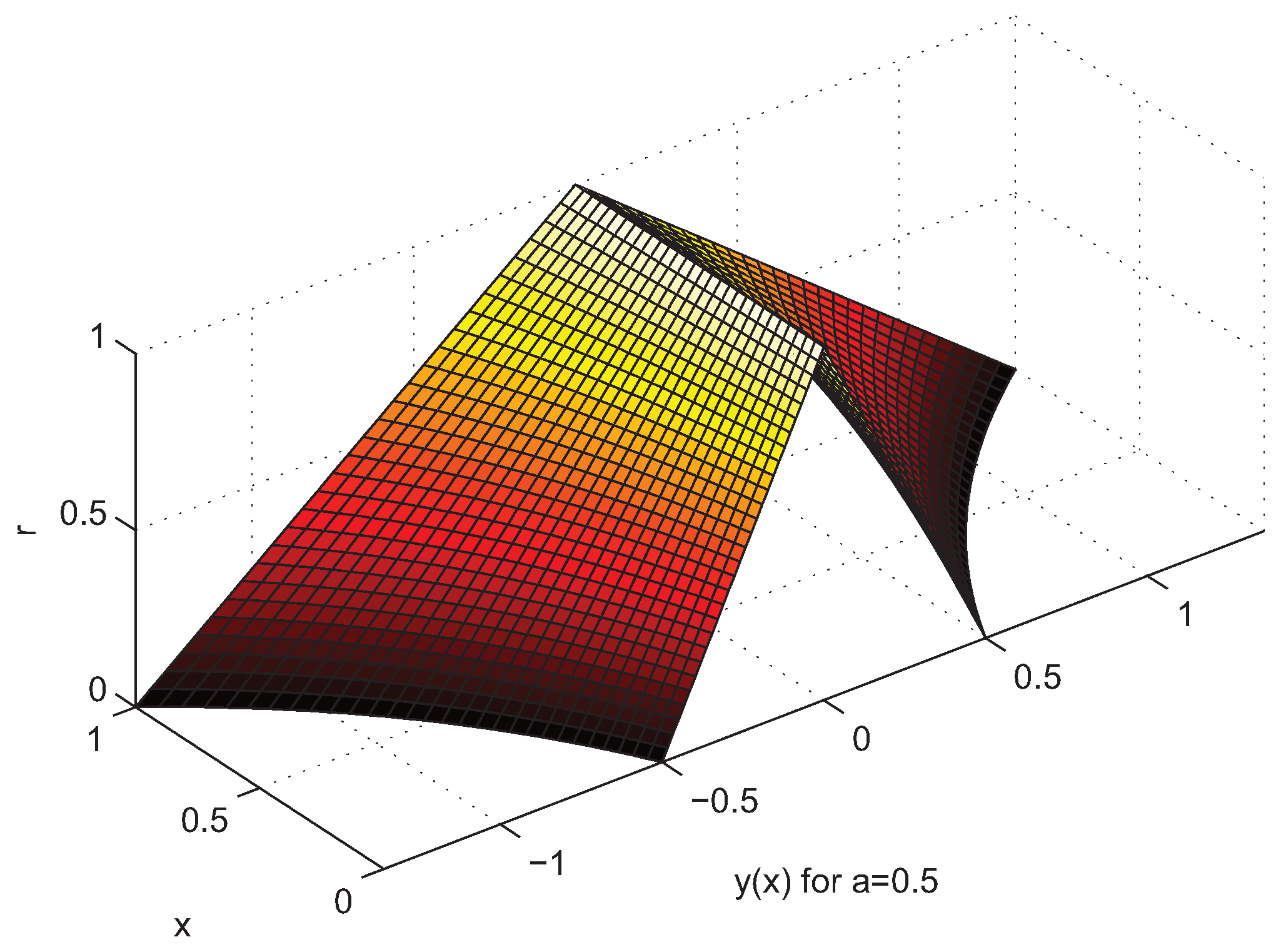
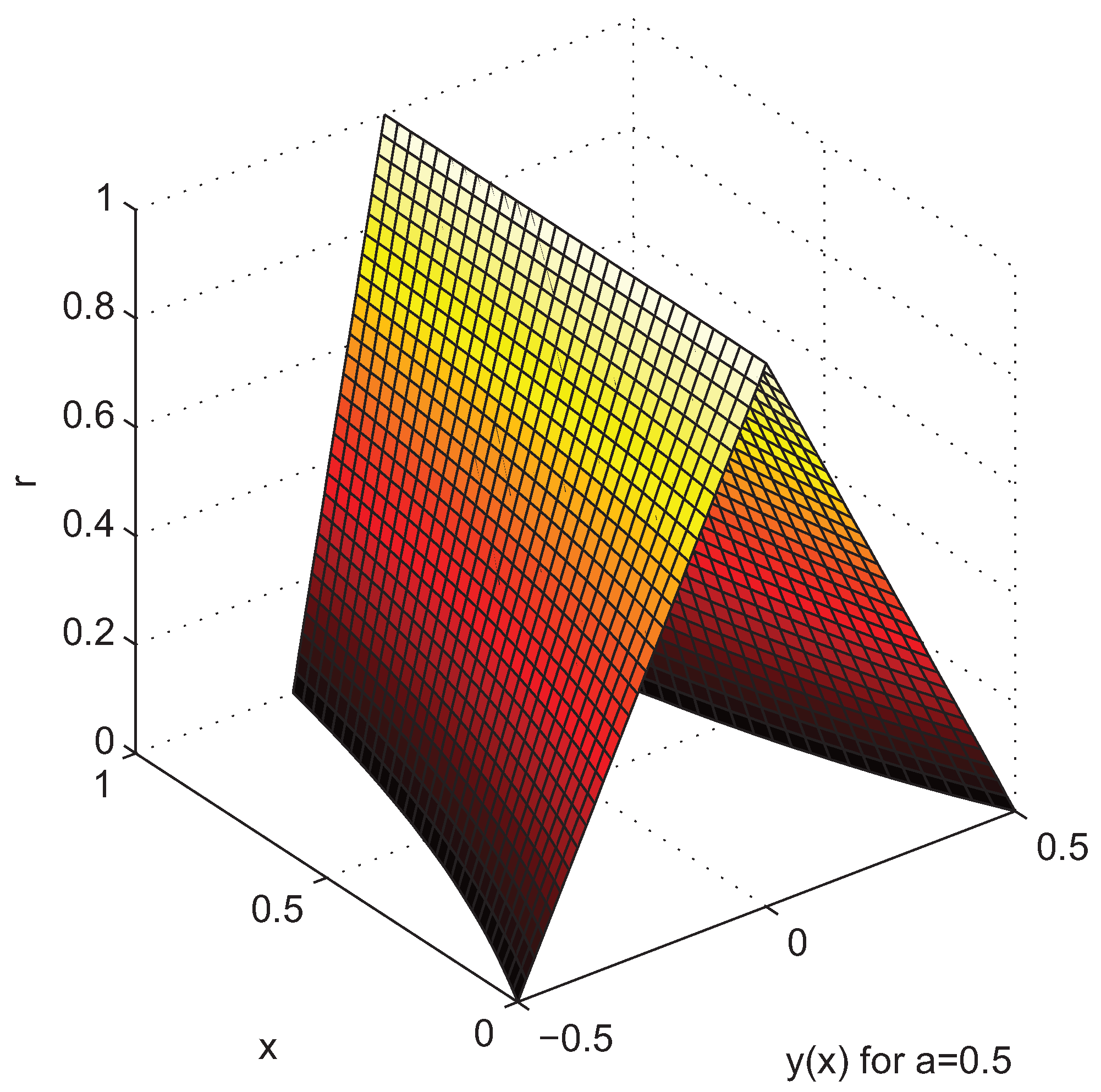
Consider the following fuzzy initial value problem

$$\left\{\begin{array}{c}{\varphi }^{\prime }(t)=\psi (t,\varphi (t)),\hfill \\ \varphi (0)=(\underline{\varphi }(0,r),\overline{\varphi }(0,r)),0<r\le 1\hfill \end{array}\right.$$

(38)

where $\psi (t,\varphi (t))$ is a fuzzy function. The fuzzy function $\psi (t,\varphi (t))$ is the mapping of $\psi :R\times E\to E$. By utilizing FST method, we obtain

$$\mathit{S}[{\varphi }^{\prime }(t)]=\mathit{S}[\psi (t,\varphi (t))]$$

(39)

The resolving process of Equation (39) is based on the following cases.

Case 1: Assume that the ${\varphi }^{\prime }(t)$ is (i)-differentiable. Based on the Theorem 4 we extract

$${\varphi }^{\prime }(t)=({\underline{\varphi }}^{\prime }(t,r),{\overline{\varphi }}^{\prime }(t,r))$$

(40)

$$\mathit{S}[{\varphi }^{\prime }(t)]=(\frac{1}{B}\odot \mathit{S}[\varphi (t)])\ominus \frac{1}{B}\varphi (0)$$

(41)

Equation (41) can be displayed as following relation

$$\left\{\begin{array}{c}\mathit{S}[\underline{\psi }(t,\varphi (t),r)]=\frac{1}{B}\mathit{S}[\underline{\varphi }(t,r)]-\frac{1}{B}\underline{\varphi }(0,\alpha )\\ \mathit{S}[\overline{\psi }(t,\varphi (t),r)]=\frac{1}{B}\mathit{S}[\overline{\varphi }(t,r)]-\frac{1}{B}\overline{\varphi }(0,r)\end{array}\right.$$

(42)

where

$$\left\{\begin{array}{c}\underline{\psi }(t,\varphi (t),r)=min\left\{\psi (t,B)\right|B\in (\underline{\varphi }(t,r),\overline{\varphi }(t,r))\}\\ \overline{\psi }(t,\varphi (t),r)=max\left\{\psi (t,B)\right|B\in (\underline{\varphi }(t,r),\overline{\varphi }(t,r))\}\end{array}\right.$$

(43)

Accordingly, Equation (43) can be resolved on the basis of the following assumptions

$$\mathit{S}[\underline{\varphi }(t,r)]=U_1(B,r)$$

(44)

$$\mathit{S}[\overline{\varphi }(t,r)]=U_2(B,r)$$

(45)

where $U_1(B,r)$, as well as $U_2(B,r)$ are the solutions of the Equation (43). By applying inverse Sumudu transform, $\underline{\varphi }(t,r)$ as well as $\overline{\varphi }(t,r)$ are computed as

$$\underline{\varphi }(t,r)={\mathit{S}}^{-1}[U_1(B,r)]$$

(46)

$$\overline{\varphi }(t,r)={\mathit{S}}^{-1}[U_2(B,r)]$$

(47)

Case 2: Assume that the ${\varphi }^{\prime }(t)$ is (ii)-differentiable. Based on the Theorem 4 we extract

$${\varphi }^{\prime }(t)=({\overline{\varphi }}^{\prime }(t,r),{\underline{\varphi }}^{\prime }(t,r))$$

(48)

$$\mathit{S}[{\varphi }^{\prime }(t)]=(\frac{-1}{B}\odot \varphi (0))\ominus (\frac{-1}{B}\odot \mathit{S}[\varphi (t)])$$

(49)

Equation (49) can be displayed as following relation

$$\left\{\begin{array}{c}\mathit{S}[\underline{\psi }(t,\varphi (t),r)]=\frac{1}{B}\mathit{S}[\underline{\varphi }(t,r)]-\frac{1}{B}\underline{\varphi }(0,r)\\ \mathit{S}[\overline{\psi }(t,\varphi (t),r)]=\frac{1}{B}\mathit{S}[\overline{\varphi }(t,r)]-\frac{1}{B}\overline{\varphi }(0,r)\end{array}\right.$$

(50)

where

$$\left\{\begin{array}{c}\underline{\psi }(t,\varphi (t),r)=min\left\{\psi (t,B)\right|B\in (\underline{\varphi }(t,r),\overline{\varphi }(t,r))\}\\ \overline{\psi }(t,\varphi (t),r)=max\left\{\psi (t,B)\right|B\in (\underline{\varphi }(t,r),\overline{\varphi }(t,r))\}\end{array}\right.$$

(51)

Accordingly, Equation (51) can be resolved on the basis of the following assumptions

$$\begin{array}{c}\mathit{S}(\underline{\varphi }(t,r)=V_1(B,r)\\ \mathit{S}(\overline{\varphi }(t,r)=V_2(B,r)\end{array}$$

(52)

where $V_1(B,r)$, and $V_2(B,r)$ are the solutions of the Equation (51). By applying inverse Sumudu transform, $\underline{\varphi }(t,r)$ as well as $\overline{\varphi }(t,r)$ are computed as

$$\begin{array}{c}\underline{\varphi }(t,r)={\mathit{S}}^{-1}[V_1(B,r)]\\ \overline{\varphi }(t,r)={\mathit{S}}^{-1}[V_2(B,r)]\end{array}$$

(53)

5. Examples

The following examples have been used to narrate the methodology proposed in this paper.

Example 1.

A tank with a heating system is displayed in Figure 1, where $\tilde{R}=0.5$, the thermal capacitance is $\tilde{C}=2$ also the temperature is ψ. The model is formulated as follows [13,32],

$$\left\{\begin{array}{l}{\varphi }^{\prime }(t)=-\frac{1}{\tilde{R}\tilde{C}}\varphi (t),0\le t\le T\\ \varphi (0)=(\underline{\varphi }(0,r),\overline{\varphi }(0,r))\end{array}\right.$$

(54)

Figure 1. Thermal system.

By utilizing the FST method, we obtain

$$\mathit{S}[{\varphi }^{\prime }(t)]=\mathit{S}[-\varphi (t)]$$

(55)

$$\mathit{S}[{\varphi }^{\prime }(t)]={\int }_0^{\infty }{\varphi }^{\prime }(Bt)\odot e^{-t}dt$$

(56)

where $0\le B<K$. If $\varphi (t)$ is (i)-differentiable and case 1 holds, we extract

$$\mathit{S}[{\varphi }^{\prime }(t)]=\frac{1}{B}\odot (\mathit{S}[\varphi (t)]\ominus \varphi (0))=\frac{1}{B}\mathit{S}[\varphi (t)]\ominus \frac{1}{B}\varphi (0)$$

(57)

Therefore

$$-\mathit{S}[\varphi (t)]=\frac{1}{B}\mathit{S}[\varphi (t)]\ominus \frac{1}{B}\varphi (0)$$

(58)

Based on the Equation (42), we have

$$\left\{\begin{array}{c}-\mathit{S}[\overline{\varphi }(t,r)]=\frac{1}{B}\mathit{S}[\underline{\varphi }(t,r)]-\frac{1}{B}\underline{\varphi }(0,r)\\ -\mathit{S}[\underline{\varphi }(t,r)]=\frac{1}{B}\mathit{S}[\overline{\varphi }(t,r)]-\frac{1}{B}\overline{\varphi }(0,r)\end{array}\right.$$

(59)

Therefore, the solution of Equation (59) is as follows

$$\left\{\begin{array}{c}\mathit{S}[\overline{\varphi }(t,r)]=(\frac{-1}{B^2-1})\overline{\varphi }(0,r)+(\frac{B}{B^2-1})\underline{\varphi }(0,r)\\ \mathit{S}[\underline{\varphi }(t,r)]=(\frac{-1}{B^2-1})\underline{\varphi }(t,r)+(\frac{B}{B^2-1})\overline{\varphi }(0,r)\end{array}\right.$$

(60)

By utilizing the inverse Sumudu transform we have

$$\left\{\begin{array}{c}\mathit{S}[\overline{\varphi }(t,r)]=\overline{\varphi }(0,r){\mathit{S}}^{-1}(\frac{-1}{B^2-1})+\underline{\varphi }(0,r){\mathit{S}}^{-1}(\frac{B}{B^2-1})\\ \mathit{S}[\underline{\varphi }(t,r)]=\underline{\varphi }(0,r){\mathit{S}}^{-1}(\frac{-1}{B^2-1})+\overline{\varphi }(0,r){\mathit{S}}^{-1}(\frac{B}{B^2-1})\end{array}\right.$$

(61)

where

$$\left\{\begin{array}{c}\overline{\varphi }(t,r)=e^t(\frac{\overline{\varphi }(0,r)-\underline{\varphi }(0,r)}{2})+e^{-t}(\frac{\overline{\varphi }(0,r)+\underline{\varphi }(0,r)}{2})\\ \underline{\varphi }(t,r)=e^t(\frac{\underline{\varphi }(0,r)-\overline{\varphi }(0,r)}{2})+e^{-t}(\frac{\underline{\varphi }(0,r)+\overline{\varphi }(0,r)}{2})\end{array}\right.$$

(62)

Now if $\varphi (t)$ be (ii)-differentiable and case 2 holds, we have

$$\mathit{S}[{\varphi }^{\prime }(t)]=(\frac{-1}{B}\mathit{S}[\varphi (t)])\ominus (\frac{-1}{B}\varphi (0))$$

(63)

Hence

$$-\mathit{S}[\varphi (t)]=(\frac{-1}{B}\mathit{S}[\varphi (t)])\ominus (\frac{-1}{B}\varphi (0))$$

(64)

Based on the above relations, Equation (54) can be written as follows

$$\left\{\begin{array}{c}-\mathit{S}[\underline{\varphi }(t,r)]=\frac{1}{B}\mathit{S}[\underline{\varphi }(t,r)]-\frac{1}{B}\underline{\varphi }(0,r)\\ -\mathit{S}[\overline{\varphi }(t,r)]=\frac{1}{B}\mathit{S}[\overline{\varphi }(t,r)]-\frac{1}{B}\overline{\varphi }(0,r)\end{array}\right.$$

(65)

So, the solution of Equation (65) is displayed as

$$\left\{\begin{array}{c}\mathit{S}[\underline{\varphi }(t,r)]=\underline{\varphi }(0,r)(\frac{1}{B+1})\\ \mathit{S}[\overline{\varphi }(t,r)]=\overline{\varphi }(t,r)(\frac{1}{B+1})\end{array}\right.$$

(66)

By utilizing the inverse Sumudu transform, we have

$$\left\{\begin{array}{c}\underline{\varphi }(t,r)=\underline{\varphi }(0,r){\mathit{S}}^{-1}(\frac{1}{B+1})\\ \overline{\varphi }(t,r)=\overline{\varphi }(0,r){\mathit{S}}^{-1}(\frac{1}{B+1})\end{array}\right.$$

(67)

where

$$\left\{\begin{array}{c}\underline{\varphi }(t,r)=e^{-t}\underline{\varphi }(0,r)\\ \overline{\varphi }(t,r)=e^{-t}\overline{\varphi }(0,r)\end{array}\right.$$

(68)

If the initial condition be a symmetric triangular fuzzy number as $\varphi (0)=(-a(1-r),a(1-r)),$ then the following cases will hold

Case 1:

$$\left\{\begin{array}{c}\underline{\varphi }(t,r)=e^t(-a(1-r))\\ \overline{\varphi }(t,r)=e^t(a(1-r))\end{array}\right.$$

(69)

Case 2:

$$\left\{\begin{array}{c}\underline{\varphi }(t,r)=e^{-t}(-a(1-r))\\ \overline{\varphi }(t,r)=e^{-t}(a(1-r))\end{array}\right.$$

(70)

Corresponding solution plots are displayed in Figure 2 and Figure 3. Corresponding error plots are shown in Figure 4. These errors are the differences of the exact and the approximation solutions for two different methods: FST and Average Euler method [33]. FST is more accurate than the Average Euler method.

Figure 2. The solution of fuzzy differential equations (FDE) under case 1 consideration.

Figure 3. The solution of FDE under case 2 consideration.

Figure 4. The lower and upper bounds of absolute errors.

Example 2.

A tank system is displayed in Figure 5. Suppose $I=t+1$ is inflow disturbances of the tank that generates vibration in liquid level ϕ, also $H=1$ is the flow obstruction, which can be curbed utilizing the valve. $Q=1$ is the cross section of the tank. The liquid level is illustrated as following relation [34],

$$\left\{\begin{array}{l}{\varphi }^{\prime }(t)=-\frac{1}{QH}\varphi (t)+\frac{I}{Q},0\le t\le T\\ \varphi (0)=(\underline{\varphi }(0,r),\overline{\varphi }(0,r))\end{array}\right.$$

(71)

Figure 5. Liquid tank system.

By utilizing the FST method we obtain

$$-\mathit{S}[\varphi (t)]=(\frac{1}{B}\odot \mathit{S}[\varphi (t)])\ominus (\frac{1}{B}\mathit{S}[\varphi (0)])$$

(72)

$$\mathit{S}[{\varphi }^{\prime }(t)]({\int }_{a_1}^{\infty }{\varphi }^{\prime }(Bt)e^{-t}dt$$

(73)

The following relation is extracted by taking into consideration case 2

$$\mathit{S}[{\varphi }^{\prime }(t)]=(\frac{-1}{B}\odot \mathit{S}[\varphi (t)])\ominus (\frac{-1}{B}\mathit{S}[\varphi (0)])$$

(74)

So

$$-\mathit{S}[\varphi (t)]+\mathit{S}[t]+\mathit{S}[1]=(\frac{-1}{B}\odot \mathit{S}[\varphi (t)])\ominus (\frac{-1}{B}\mathit{S}[\varphi (0)])$$

(75)

Based on the Equation (42), we have

$$\left\{\begin{array}{c}-\mathit{S}[\underline{\varphi }(t,r)]+\mathit{S}[t]+\mathit{S}[1]=\frac{1}{B}\mathit{S}[\underline{\varphi }(t,r)]-\frac{1}{B}\underline{\varphi }(0,r)\\ -\mathit{S}[\overline{\varphi }(t,r)]+\mathit{S}[t]+\mathit{S}[1]=\frac{1}{B}\mathit{S}[\overline{\varphi }(t,r)]-\frac{1}{B}\overline{\varphi }(0,r)\end{array}\right.$$

(76)

Therefore, the solution of Equation (76) is extracted as

$$\left\{\begin{array}{l}\mathit{S}[\underline{\varphi }(t,r)]=\mathit{S}[t]+\mathit{S}[1]+\frac{-1}{B}\mathit{S}[\underline{\varphi }(t,r)]-\frac{1}{B}\underline{\varphi }(0,r)\\ \mathit{S}[\overline{\varphi }(t,r)]=\mathit{S}[t]+\mathit{S}[1]+\frac{1}{B}\mathit{S}[\overline{\varphi }(t,r)]-\frac{1}{B}\overline{\varphi }(0,r)\end{array}\right.$$

(77)

hence,

$$\left\{\begin{array}{c}\mathit{S}[\underline{\varphi }(t,r)]=(\frac{1}{B+1})\underline{\varphi }(0,r)+B\\ \mathit{S}[\overline{\varphi }(t,r)]=(\frac{1}{B+1})\overline{\varphi }(t,r)+B\end{array}\right.$$

(78)

By utilizing the inverse Sumudu transform, we obtain

$$\left\{\begin{array}{c}\underline{\varphi }(t,r)=\underline{\varphi }(0,r){\mathit{S}}^{-1}(\frac{1}{B+1})+{\mathit{S}}^{-1}(B)\\ \overline{\varphi }(t,r)=\overline{\varphi }(0,r){\mathit{S}}^{-1}(\frac{1}{B+1})+{\mathit{S}}^{-1}(B)\end{array}\right.$$

(79)

where

$$\left\{\begin{array}{c}\underline{\varphi }(t,r)=e^{-t}\underline{\varphi }(0,r)+t\\ \overline{\varphi }(t,r)=e^{-t}\overline{\varphi }(0,r)+t\end{array}\right.$$

(80)

If the initial condition is taken to be a symmetric triangular fuzzy number as $\varphi (0)=(-a(1-r),a(1-r))$, so

$$\left\{\begin{array}{l}\underline{\varphi }(t,r)=e^{-t}(-a(1-r))+t\\ \overline{\varphi }(t,r)=e^{-t}(a(1-r))+t\end{array}\right.$$

(81)

Corresponding solution plot is displayed in Figure 6.

Figure 6. The solution of FDE under case 2 consideration.

Example 3.

The nuclear decay equation can be described as [30],

$$\left\{\begin{array}{l}{N}^{\prime }(t)=-\lambda N(t)\\ N(0)=(\underline{N}(0,r),\overline{N}(0,r))\end{array}\right.$$

(82)

where $N(t)$ is considered to be the number of radionuclides present, λ is state as the decay constant, also $N_0$ is taken to be the initial number of radionuclides. Let $N_0$ be a fuzzy number. By utilizing the FST method the following outcomes can be demonstrated

$$\mathit{S}[N^{\prime }(t)]=\mathit{S}[-\lambda N(t)]=-\lambda \mathit{S}[N(t)]$$

(83)

$$\mathit{S}[N^{\prime }(t)]={\int }_a^{\infty }{N}^{\prime }(st)e^{-t}dt$$

(84)

If $N(t)$ is (ii)-differentiable and case 2 holds, we obtain

$$\mathit{S}[N^{\prime }(t)]=(\frac{-1}{B}\mathit{S}[N(t)])\ominus (\frac{-1}{B}N(0))$$

(85)

Therefore

$$-\lambda \mathit{S}[N(t)]=(\frac{-1}{B}\mathit{S}[N(t)])\ominus (\frac{-1}{B}N(0))$$

(86)

According to Equation (42), we will have the below mentioned relation

$$\left\{\begin{array}{c}-\lambda \mathit{S}[\underline{N}(t,r)]=\frac{1}{B}\mathit{S}[\underline{N}(t,r)]-\frac{1}{B}\underline{N}(0,r)\\ -\lambda \mathit{S}[\overline{N}(t,r)]=\frac{1}{B}\mathit{S}[\overline{N}(t,r)]-\frac{1}{B}\overline{N}(0,r)\end{array}\right.$$

(87)

Hence, the solution of Equation (87) is as follows:

$$\left\{\begin{array}{c}\mathit{S}[\underline{N}(t,r)](\lambda -\frac{1}{B})=\frac{1}{B}\underline{N}(0,r)\\ \mathit{S}[\overline{N}(t,r)](\lambda -\frac{1}{B})=\frac{1}{B}\overline{N}(t,r)\end{array}\right.$$

(88)

Thus we extract

$$\left\{\begin{array}{c}\mathit{S}[\underline{N}(t,r)]=\frac{1}{-\lambda B+1}\underline{N}(0,r)\\ \mathit{S}[\overline{N}(t,r)]=\frac{1}{-\lambda B+1}\overline{N}(t,r)\end{array}\right.$$

(89)

So, by utilizing the inverse Sumudu transform the following outcomes can be observed

$$\left\{\begin{array}{c}\underline{N}(t,r)=\underline{N}(0,r){\mathit{S}}^{-1}(\frac{1}{-\lambda B+1})\\ \overline{N}(t,r)=\overline{N}(0,r){\mathit{S}}^{-1}(\frac{1}{-\lambda B+1})\end{array}\right.$$

(90)

where

$$\left\{\begin{array}{c}\underline{N}(t,r)=e^{-\lambda t}\underline{N}(0,r)\\ \overline{N}(t,r)=e^{-\lambda t}\overline{N}(0,r)\end{array}\right.$$

(91)

Let $\lambda =1$ and $N_0=(1,2,5)$, then

$$\left\{\begin{array}{c}\underline{N}(0,r)=(1+r)\\ \overline{N}(0,r)=(5-3r)\end{array}\right.$$

(92)

So

$$\left\{\begin{array}{c}\underline{N}(t,r)=e^{-t}(1+r)\\ \overline{N}(t,r)=e^{-t}(5-3r)\end{array}\right.$$

(93)

Corresponding solution plot is displayed in Figure 7.

Figure 7. The solution of the nuclear decay equation under case 2 consideration.

6. Conclusions

In this paper, the utilization of FST results in the solution of the first order FDEs in such a manner that it is clarified by using the notion of strongly generalized differentiability. By implementing the methodology of FST, the FDE reduces to an algebraic problem. Some theorems are given to illustrate the properties of the FST. The novel method is validated by three real examples. Numerical experiments along with comparisons demonstrate the excellent behavior of the proposed method. This work makes a significant contribution in initializing a superior starting point for such extensions. Future work involves studying the application of this method in solving FDEs where the uncertainties are in the form of Z-numbers.

References

- Zwillinger, D. Handbook of Differential Equations; Gulf Professional Publishing: Houston, TX, USA, 1998. [Google Scholar]
- Khalili Golmankhaneh, A.; Porghoveh, N.; Baleanu, D. Mean square solutions of second-order random differential equations by using Homotopy analysis method. Rom. Rep. Phys. 2013, 65, 350–361. [Google Scholar]
- Buckley, J.J.; Eslami, E.; Feuring, T. Fuzzy Mathematics in Economics and Engineering; Physica-Verlag: Heidelberg, Germany, 2002. [Google Scholar]
- Diamond, P.; Kloeden, P. Metric Spaces of Fuzzy Sets: Theory and Applications; World Scientific: Singapore, 1994. [Google Scholar]
- Kloeden, P. Remarks on Peano-like theorems for fuzzy differential equations. Fuzzy Set Syst. 1991, 44, 161–164. [Google Scholar] [CrossRef]
- Jafari, R.; Yu, W. Fuzzy Control for Uncertainty Nonlinear Systems with Dual Fuzzy Equations. J. Intell. Fuzzy Syst. 2015, 29, 1229–1240. [Google Scholar] [CrossRef]
- Jafari, R.; Yu, W. Fuzzy Differential Equation for Nonlinear System Modeling with Bernstein Neural Networks. IEEE Access 2016. [Google Scholar] [CrossRef]
- Jafari, R.; Yu, W. Uncertainty Nonlinear Systems Modeling with Fuzzy Equations. Math. Probl. Eng. 2017. [Google Scholar] [CrossRef]
- Jafarian, A.; Jafari, R. Approximate solutions of dual fuzzy polynomials by feed-back neural networks. J. Soft Comput. Appl. 2012. [Google Scholar] [CrossRef]
- Jafari, R.; Yu, W.; Li, X.; Razvarz, S. Numerical Solution of Fuzzy Differential Equations with Z-numbers Using Bernstein Neural Networks. Int. J. Comput. Int. Sys. 2017, 10, 1226–1237. [Google Scholar] [CrossRef]
- Jafari, R.; Yu, W.; Li, X. Numerical solution of fuzzy equations with Z-numbers using neural networks. Intell. Autom. Soft Comput. 2017, 1–7. [Google Scholar] [CrossRef]
- Friedman, M.; Ming, M.; Kandel, A. Numerical solution of fuzzy differential and integral equations. Fuzzy Set Syst. 1999, 106, 35–48. [Google Scholar] [CrossRef]
- Allahviranloo, T.; Ahmadi, M.B. Fuzzy Laplace Transform. Soft Comput. 2010, 14, 235–243. [Google Scholar] [CrossRef]
- Ding, Z.; Ma, M.; Kandel, A. Existence of the solutions of fuzzy differential equations with parameters. Inf. Sci. 1997, 99, 205–217. [Google Scholar] [CrossRef]
- Truong, V.A.; Ngo, V.H.; Nguyen, D.P. Global existence of solutions for interval-valued integro-differential equations under generalized H-differentiability. Adv. Differ. Equ. 2013, 1, 217–233. [Google Scholar] [CrossRef]
- Asiru, M.A. Further properties of the Sumudu transform and its applications. Int. J. Math. Educ. Sci. Tech. 2002, 33, 441–449. [Google Scholar] [CrossRef]
- Belgacem, F.B.M.; Karaballi, A.A.; Kalla, S.L. Analytical investigations of the Sumudu transform and applications to integral production equations. Math. Probl. Eng. 2003, 103, 103–118. [Google Scholar] [CrossRef]
- Deakin, M.A.B. The Sumudu transform and the Laplace transform. Int. J. Math. Educ. Sci. Technol. 1997, 28, 159–160. [Google Scholar] [CrossRef]
- Eltayeb, H.; Kilicman, A. A note on the Sumudu transforms and differential equations. Appl. Math. Sci. 2010, 4, 1089–1098. [Google Scholar]
- Srivastava, H.M.; Khalili Golmankhaneh, A.; Baleanu, D.; Yang, X.J. Local Fractional Sumudu Transform with Application to IVPs on Cantor Sets. Abstr. Appl. Anal. 2014. [Google Scholar] [CrossRef]
- Abdul Rahman, N.A.; Ahmad, M.Z. Fuzzy Sumudu transform for solving fuzzy partial differential equations. J. Nonlinear Sci. Appl. 2016, 9, 3226–3239. [Google Scholar] [CrossRef]
- Belgacem, F.B.M.; Karaballi, A.A. Sumudu transform fundamental properties investigations and applications. J. Appl. Math. Stoch. Anal. 2006. [Google Scholar] [CrossRef]
- Liu, Y.; Chen, W. A new iterational method for ordinary equations using Sumudu transform. Adv. Anal. 2016. [Google Scholar] [CrossRef]
- Jafari, R.; Razvarz, S. Solution of Fuzzy Differential Equations using Fuzzy Sumudu Transforms. IEEE Int. Conf. Innov. Intell. Syst. Appl. 2017. [Google Scholar] [CrossRef]
- Bede, B.; Stefanini, L. Generalized differentiability of fuzzy-valued functions. Fuzzy Set Syst. 2013, 230, 119–141. [Google Scholar] [CrossRef]
- Seikkala, S. On the fuzzy initial value problem. Fuzzy Set Syst. 1987, 24, 319–330. [Google Scholar] [CrossRef]
- Puri, M.L.; Ralescu, D. Fuzzy random variables. J. Math. Anal. Appl. 1986, 114, 409–422. [Google Scholar] [CrossRef]
- Wu, H.-C. The improper fuzzy Riemann integral and its numerical integration. Inform. Sci. 1999, 111, 109–137. [Google Scholar] [CrossRef]
- Bede, B.; Gal, S.G. Generalizations of the differentiability of fuzzy-number-valued functions with applications to fuzzy differential equations. Fuzzy Set Syst. 2005, 151, 581–599. [Google Scholar] [CrossRef]
- Bede, B.; Rudas, I.J.; Bencsik, A.L. First order linear fuzzy differential equations under generalized differentiability. Inf. Sci. 2006, 177, 1648–1662. [Google Scholar] [CrossRef]
- Chalco-Cano, Y.; Roman-Flores, H. On new solutions of fuzzy differential equations. Chaos Solitons Fractals 2006, 38, 112–119. [Google Scholar] [CrossRef]
- Pletcher, R.H.; Tannehill, J.C.; Anderson, D. Computational Fluid Mechanics and Heat Transfer; Taylor and Francis: Abingdon, UK, 1997. [Google Scholar]
- Tapaswini, S.; Chakraverty, S. Euler-based new solution method for fuzzy initial value problems. Int. J. Artif. Intell. Soft Comput. 2014, 4, 58–79. [Google Scholar] [CrossRef]
- Streeter, V.L.; Wylie, E.B.; Bedford, K.W. Fluid Mechanics; McGraw Hill: New York, NY, USA, 1998. [Google Scholar]
© 2018 by the authors. Licensee MDPI, Basel, Switzerland. This article is an open access article distributed under the terms and conditions of the Creative Commons Attribution (CC BY) license (http://creativecommons.org/licenses/by/4.0/).