An M/G/1 Retrial G-Queue with General Retrial Times and Working Breakdowns

Abstract

This paper considers an M/G/1 retrial G-queue with general retrial times, in which the server is subject to working breakdowns and repairs. If the system is not empty during a normal service period, the arrival of a negative customer can cause the server breakdown, and the failed server still works at a lower service rate rather than stopping the service completely. Applying the embedded Markov chain, we obtain the necessary and sufficient condition for the stability of the system. Using the supplementary variable method, we deal with the generating functions of the number of customers in the orbit. Various system performance measures are also developed. Finally, some numerical examples and a cost optimization analysis are presented.

1. Introduction

Queues with negative arrivals, called G-queues, were first introduced by Gelenbe [1]. A negative customer will vanish if it arrives to the queue when the server is down or on vacation. Negative customers cannot accumulate in a queue and do not receive services. In some cases, the arrival of a negative customer can cause the server breakdown. Queues with server breakdowns can be applied in manufacturing systems, production systems, telecommunication systems, inventory systems and computer systems. Wu and Lian [2] analyzed an M/G/1 retrial G-queue with priority under the Bernoulli vacation schedule subject to the server breakdowns and repairs. Gao and Wang [3] investigated an M/G/1 retrial G-queue with orbital search and non-persistent customers, where the server is subject to failure due to the negative arrivals. Using the matrix geometric method, Rakhee et al. [4] studied a Geo/Geo/1 G-queue with an unreliable server, where the breakdown of the server is represented due to the arrival of a negative customer. Some authors like Wang and Zhang [5], Do [6], Yang et al. [7], Peng et al. [8], Chen et al. [9] and Bhagat and Jain [10] also discussed a retrial G-queue with server breakdowns.

In the study of queueing models with server breakdowns, the underlying assumption has been that a server breakdown disrupts the service completely in the system. However, in many practical cases, the failed server still can serve a customer at a lower service rate during the breakdown period. This type of breakdown is called a working breakdown, as introduced by Kalidass and Kasturi [11], and the M/M/1 queue they analyzed can be applied to studying the behavior of the communication system or the machine replacement problem. Liu and Song [12] extended the M/M/1 queue to the M${}^X$/M/1 queue, where customers arrive in batches. Kim and Lee [13] discussed an M/G/1 queue with disasters and working breakdowns, where the system size distribution and the sojourn time distribution are obtained. Recently, Liou [14] considered the profit optimization of an M/M/1 machine repair problem with warm standbys, multiple vacations and working breakdowns. Jiang and Liu [15] investigated a GI/M/1 queue with disasters and working breakdowns in a multi-phase service environment. Using the matrix geometric method, Ma et al. [16] computed the steady-state distribution of an M/M/1 queue with multiple vacations and working breakdowns. For more queueing models with working breakdowns, readers can also refer to Li et al. [17], Liou [18], Chen et al. [19] and Yen et al. [20]. Note that the concept of working breakdown is different from the concept of working vacation introduced by Servi and Finn [21]. A working vacation is taken only when the system becomes empty, while a working breakdown can occur at any time point at which the server is busy with the service of a customer in the system. Some authors like Yi et al. [22], Yang and Wu [23], Zhang and Liu [24] and Murugan and Santhi [25] have studied a queueing system with server breakdowns and working vacations.

Retrial queues can be applied in telecommunication networks, switching systems and computer networks, and there has been an increasing interest in the analysis of retrial systems in recent years. Retrial queues are described by the feature that the arriving customers who find the server busy join the retrial orbit to try again for their requests. A review of retrial queue literature can be found in Artalejo and Corral [26] and Artalejo [27]. Retrial queueing systems with working vacations were first studied by Do [28], and the M/M/1 model is motivated by the performance analysis of a media access control function in wireless networks. For more retrial queues with working vacations, readers can refer to Jailaxmi et al. [29] and Rajadurai et al. [30,31]. The concept of working breakdown introduced by Kalidass and Kasturi [11] does make sense in real life. For example, when a computer is infected with a virus, it may still be able to perform at a slower rate. Up to now, only a few authors have discussed a single server queue with working breakdowns. To the authors’ best knowledge, there is no research work investigating a retrial queue with working breakdowns. This motivates us to deal with an M/G/1 retrial G-queue with working breakdowns in this paper, where a breakdown may occur due to the arrival of a negative customer.

A practical application example of the proposed model is referred to in the manufacturing system. Assume that a manufacturing factory has a machine shared by all units (called positive customers) of the factory, and the machine is operated by an operator. If the machine is busy, a new positive arrival will sign up on a waiting line, which corresponds to the retrial queue. Otherwise, the unit is served immediately. After the completion of a service, if there is no unit (the system is empty), the operator will turn the machine off. Otherwise, the operator will contact the next unit on the list unless another external unit arrives before the contact is made. The contact time is assumed to be generally distributed (corresponding to the general retrial time). Due to the machine problem, a machine may suddenly break down when it is running (corresponding to the negative customer arrival). The broken down machine is immediately replaced by another standby machine, which may work at a lower rate, and a repair procedure also starts. The operator will sign up the unit being in service (if any) on the waiting line, i.e., join the retrial orbit, and the service is restarted by the standby machine after some random time. As soon as the broken down machine is repaired, it is put back into service, if there are units in the system. To guarantee the service quality, the repaired machine will restart service no matter how long the standby machine has served. If the system is empty, on the other hand, the operator will turn off the repaired machine, which cannot break down. On the arrival of a unit, the operator turns on the machine immediately, and the service begins.

This paper is organized as follows. Section 2 gives a brief description of the model. Using the embedded Markov chain, the stable condition is obtained in Section 3. In Section 4, we deal with the steady state joint distribution of the server state and the number of customers in the retrial orbit. In Section 5, some numerical examples are presented to show the effect of the parameters on the system performance measures, and a cost minimization problem is also considered. Finally, Section 6 concludes the paper.

2. System Model

In this paper, we consider an M/G/1 retrial queue with two types of arrivals, where positive customers and negative customers arrive according to two independent Poisson processes with rates ${\lambda }_1$ and ${\lambda }_2$, respectively. On the arrival of a positive customer, if the server is found to be idle, the arriving positive customer occupies the server and begins its service immediately. If the server is busy, on the other hand, the arriving positive customer will join the retrial orbit. We assume that only the positive customer at the head of the orbit queue is allowed to retry access to the server at a service completion instant. The retrial time R is assumed to be generally distributed with distribution function $R\left(x\right)=1-exp\{-{\int }_0^x\alpha \left(t\right)dt\}$. On the arrival of a negative customer, if the system is not empty, the server will break down, no matter whether the server is busy or free. The positive customer being in service, if any, will join the orbit and try to restart its service after some random time. We also assume that the negative customers cannot accumulate in a queue and do not receive services. When the server breaks down, the service rate decreases, and a repair procedure starts immediately; the repair time V follows an exponential distribution with a parameter θ. The repaired server is assumed to be as good as a new server. At the end of the repair, if the server is busy, the service will be restarted. If the server is free, on the other hand, the server stays idle. Furthermore, the arriving negative customer has nothing to do with the server when the system is empty or the server is under repair. In a regular busy period, the normal service time $S_b$ follows an arbitrary distribution with distribution function $G_b\left(x\right)=1-exp\{-{\int }_0^x\mu \left(t\right)dt\}$. During a working breakdown period, the lower service time $S_v$ follows an arbitrary distribution with distribution function $G_v\left(x\right)=1-exp\{-{\int }_0^x\eta \left(t\right)dt\}$.

We assume that all of the random variables defined above are independent. Throughout the rest of the paper, we denote $\lambda ={\lambda }_1+{\lambda }_2$. For a distribution function $F\left(x\right)$, we define $\overline{F}\left(x\right)=1-F\left(x\right)$ to be the tail of $F\left(x\right)$. We also denote $\tilde{F}\left(s\right)={\int }_0^{\infty }{e}^{-sx}dF\left(x\right)$, ${\overline{F}}^{\ast }\left(s\right)={\int }_0^{\infty }{e}^{-sx}\overline{F}\left(x\right)dx$. Clearly, we have ${\overline{F}}^{\ast }\left(s\right)=\frac{1-\tilde{F}\left(s\right)}{s}$.

Let $N\left(t\right)$ represent the number of positive customers in the retrial orbit at time t and $I\left(t\right)$ denote the server state, defined as follows:

$$\begin{array}{c}\hfill \begin{array}{c}\hfill I\left(t\right)=\left\{\begin{array}{cc}0,\hfill & \mathrm{the}\mathrm{server}\mathrm{is}\mathrm{in}\mathrm{a}\mathrm{working}\mathrm{breakdown}\mathrm{period}\mathrm{at}\mathrm{time}t\mathrm{and}\mathrm{the}\mathrm{server}\mathrm{is}\mathrm{free},\hfill \\ 1,\hfill & \mathrm{the}\mathrm{server}\mathrm{is}\mathrm{in}\mathrm{a}\mathrm{working}\mathrm{breakdown}\mathrm{period}\mathrm{at}\mathrm{time}t\mathrm{and}\mathrm{the}\mathrm{server}\mathrm{is}\mathrm{busy},\hfill \\ 2,\hfill & \mathrm{the}\mathrm{server}\mathrm{is}\mathrm{in}\mathrm{a}\mathrm{working}\mathrm{breakdown}\mathrm{period}\mathrm{at}\mathrm{time}t\mathrm{and}\mathrm{the}\mathrm{server}\mathrm{is}\mathrm{free},\hfill \\ 3,\hfill & \mathrm{the}\mathrm{server}\mathrm{is}\mathrm{in}\mathrm{a}\mathrm{working}\mathrm{breakdown}\mathrm{period}\mathrm{at}\mathrm{time}t\mathrm{and}\mathrm{the}\mathrm{server}\mathrm{is}\mathrm{busy}.\hfill \end{array}\right.\end{array}\end{array}$$

At time $t\ge 0$, we define the random variable $\xi \left(t\right)$ as follows: if $I\left(t\right)$ = 0 or $I\left(t\right)$ = 2 and $N\left(t\right)>0$, $\xi \left(t\right)$ represents the elapsed retrial time; if $I\left(t\right)$ = 1, $\xi \left(t\right)$ denotes the elapsed lower service time; if $I\left(t\right)$ = 3, $\xi \left(t\right)$ stands for the elapsed normal service time. Therefore, the system can be described by a Markov process $X\left(t\right)=\left\{I\right(t),N(t),\xi (t\left)\right\}$ with state space:

$$\begin{array}{c}\hfill \mathsf{\Omega }=\left\{\right(0,0\left)\right\}\cup \left\{\right(1,0,x),x\ge 0\}\cup \left\{\right(2,0\left)\right\}\cup \left\{\right(3,0,x),x\ge 0\}\cup \left\{\right(i,n,x),i=0,1,2,3,n\ge 1,x\ge 0\}.\end{array}$$

Let {$t_n$; $n=1,2,\cdots$} be the sequence of epochs at which a service completion or a breakdown occurs and $Y_n=\{I\left(t_n^{+}\right),N\left(t_n^{+}\right)\}$. Then, the sequence of random variables {$Y_n;n\ge 1$} forms an embedded Markov chain with state space $\left\{\right(i,k),i=0,2,k\ge 0\}$.

3. Stable Condition

To develop the transition matrix of {$Y_n$; $n\ge 1$}, we introduce a few definitions:

Definition 1.

$a_k={\int }_0^{\infty }\frac{{\left({\lambda }_{1}x\right)}^k}{k!}{e}^{-{\lambda }_{1}x}{e}^{-{\lambda }_{2}x}d{G}_b\left(x\right),k\ge 0,$

which represents the probability that k positive customers arrive during $S_b$ and no negative customer arrives; we can have:

$$\begin{array}{cc}\hfill A\left(z\right)& \stackrel{▵}{=}\sum _{k=0}^{\infty }{a}_k{z}^k={\int }_0^{\infty }{e}^{-(\lambda -{\lambda }_{1}z)x}d{G}_b\left(x\right)={\tilde{G}}_b(\lambda -{\lambda }_{1}z),A\left(1\right)={\tilde{G}}_b\left({\lambda }_2\right),\hfill \\ \hfill A^{\prime }\left(1\right)& ={\lambda }_1{\int }_0^{\infty }x{e}^{-{\lambda }_{2}x}d{G}_b\left(x\right),A^{\prime \prime }\left(1\right)={\lambda }_1^2{\int }_0^{\infty }{x}^2{e}^{-{\lambda }_{2}x}d{G}_b\left(x\right).\hfill \end{array}$$

Definition 2.

$b_k={\int }_0^{\infty }\frac{{\left({\lambda }_{1}x\right)}^k}{k!}{e}^{-{\lambda }_{1}x}{\lambda }_2{e}^{-{\lambda }_{2}x}{\overline{G}}_b\left(x\right)dx,k\ge 0,$

which explains the probability that k positive customers arrive before the negative customer arrives and no services complete; we can get:

$$\begin{array}{cc}\hfill B\left(z\right)& \stackrel{▵}{=}\sum _{k=0}^{\infty }{b}_k{z}^k={\int }_0^{\infty }{\lambda }_2{e}^{-(\lambda -{\lambda }_{1}z)x}{\overline{G}}_b\left(x\right)dx=\frac{{\lambda }_2}{\lambda -{\lambda }_{1}z}\left(1-A\left(z\right)\right),B\left(1\right)=1-A\left(1\right),\hfill \\ \hfill B^{\prime }\left(1\right)& =\frac{{\lambda }_1}{{\lambda }_2}\left(1-A\left(1\right)\right)-A^{\prime }\left(1\right),B^{\prime \prime }\left(1\right)=2{\left(\frac{{\lambda }_1}{{\lambda }_2}\right)}^2\left(1-A\left(1\right)\right)-2\frac{{\lambda }_1}{{\lambda }_2}{A}^{\prime }\left(1\right)-A^{\prime \prime }\left(1\right).\hfill \end{array}$$

Definition 3.

$c_k={\int }_0^{\infty }\frac{{\left({\lambda }_{1}x\right)}^k}{k!}{e}^{-{\lambda }_{1}x}{e}^{-\theta x}d{G}_v\left(x\right),k\ge 0,$

which represents the probability that $V\ge S_v$ and k positive customers arrive during $S_v$; we can obtain:

$$\begin{array}{cc}\hfill C\left(z\right)& \stackrel{▵}{=}\sum _{k=0}^{\infty }{c}_k{z}^k={\int }_0^{\infty }{e}^{-\left(\theta +{\lambda }_1(1-z)\right)x}d{G}_v\left(x\right)={\tilde{G}}_v\left(\theta +{\lambda }_1(1-z)\right),C\left(1\right)={\tilde{G}}_v\left(\theta \right),\hfill \\ \hfill C^{\prime }\left(1\right)& ={\lambda }_1{\int }_0^{\infty }x{e}^{-\theta x}d{G}_v\left(x\right),C^{\prime \prime }\left(1\right)={\lambda }_1^2{\int }_0^{\infty }{x}^2{e}^{-\theta x}d{G}_v\left(x\right).\hfill \end{array}$$

Definition 4.

$d_k={\int }_0^{\infty }\frac{{\left({\lambda }_{1}x\right)}^k}{k!}{e}^{-{\lambda }_{1}x}\theta e^{-\theta x}{\overline{G}}_v\left(x\right)dx,k\ge 0,$

which explains the probability that $V<S_v$ and k positive customers arrive during V; we can derive:

$$\begin{array}{cc}\hfill D\left(z\right)& \stackrel{▵}{=}\sum _{k=0}^{\infty }{d}_k{z}^k=\theta {\overline{G}}_v^{\ast }\left(\theta +{\lambda }_1(1-z)\right)=\frac{\theta }{\theta +{\lambda }_1(1-z)}\left[1-C\left(z\right)\right],D\left(1\right)=1-C\left(1\right),\hfill \\ \hfill D^{\prime }\left(1\right)& =\frac{{\lambda }_1}{\theta }\left(1-C\left(1\right)\right)-C^{\prime }\left(1\right),D^{\prime \prime }\left(1\right)=2{\left(\frac{{\lambda }_1}{\theta }\right)}^2\left(1-C\left(1\right)\right)-2\frac{{\lambda }_1}{\theta }{C}^{\prime }\left(1\right)-C^{\prime \prime }\left(1\right).\hfill \end{array}$$

Definition 5.

$u_k={\sum }_{j=0}^k{d}_j{a}_{k-j},k\ge 0,$

which represents the probability that $V<S_v$ and k positive customers arrive during V plus $S_b$; we can have:

$$\begin{array}{cc}\hfill U\left(z\right)& \stackrel{▵}{=}\sum _{k=0}^{\infty }{u}_k{z}^k=D\left(z\right)A\left(z\right),U\left(1\right)=D\left(1\right)A\left(1\right),\hfill \\ \hfill U^{\prime }\left(1\right)& =D^{\prime }\left(1\right)A\left(1\right)+D\left(1\right)A^{\prime }\left(1\right),U^{\prime \prime }\left(1\right)=D^{\prime \prime }\left(1\right)A\left(1\right)+2D^{\prime }\left(1\right)A^{\prime }\left(1\right)+D\left(1\right)A^{\prime \prime }\left(1\right).\hfill \end{array}$$

Definition 6.

$v_k={\sum }_{j=0}^k{d}_j{b}_{k-j},k\ge 0,$

which explains the probability that $V<S_v$ and the new started service does not complete before the negative customer arrives, and k positive customers arrive during the whole period; we can get:

$$\begin{array}{cc}\hfill V\left(z\right)& \stackrel{▵}{=}\sum _{k=0}^{\infty }{v}_k{z}^k=D\left(z\right)B\left(z\right),V\left(1\right)=D\left(1\right)B\left(1\right),\hfill \\ \hfill V^{\prime }\left(1\right)& =D^{\prime }\left(1\right)B\left(1\right)+D\left(1\right)B^{\prime }\left(1\right),V^{\prime \prime }\left(1\right)=D^{\prime \prime }\left(1\right)B\left(1\right)+2D^{\prime }\left(1\right)B^{\prime }\left(1\right)+D\left(1\right)B^{\prime \prime }\left(1\right).\hfill \end{array}$$

Using the lexicographical sequence for the states, the transition probability matrix of {$Y_n;n\ge 1$} can be written as the block-Jacobi matrix:

$$P=\left(\begin{array}{ccccc}{W}_0& W_1& W_2& W_3& \cdots \\ A_0& A_1& A_2& A_3& \cdots \\ & A_0& A_1& A_2& \cdots \\ & & A_0& A_1& \cdots \\ & & & \ddots & \ddots \end{array}\right),$$

where:

$$\begin{array}{cc}\hfill W_0& =\left(\begin{array}{cc}{\displaystyle \frac{{\lambda }_1}{{\lambda }_1+\theta }}{c}_0& {\displaystyle \frac{{\lambda }_1}{{\lambda }_1+\theta }}{u}_0+{\displaystyle \frac{\theta }{{\lambda }_1+\theta }}\\ 0& a_0\end{array}\right),W_k=\left(\begin{array}{cc}{\displaystyle \frac{{\lambda }_1}{{\lambda }_1+\theta }}(c_k+v_{k-1})& {\displaystyle \frac{{\lambda }_1}{{\lambda }_1+\theta }}{u}_k\\ b_{k-1}& a_k\end{array}\right),k\ge 1,\hfill \\ \hfill A_0& =\left(\begin{array}{cc}\tilde{R}\left({\lambda }_1\right)c_0& \tilde{R}\left({\lambda }_1\right)u_0\\ 0& \tilde{R}\left(\lambda \right)a_0\end{array}\right),A_1=\left(\begin{array}{cc}\tilde{R}\left({\lambda }_1\right)(c_1+v_0)+{\lambda }_1{\overline{R}}^{\ast }\left({\lambda }_1\right)c_0& \tilde{R}\left({\lambda }_1\right)u_1+{\lambda }_1{\overline{R}}^{\ast }\left({\lambda }_1\right)u_0\\ \tilde{R}\left(\lambda \right)b_0+{\lambda }_2{\overline{R}}^{\ast }\left(\lambda \right)& \tilde{R}\left(\lambda \right)a_1+{\lambda }_1{\overline{R}}^{\ast }\left(\lambda \right)a_0\end{array}\right),\hfill \\ \hfill A_k& =\left(\begin{array}{cc}\tilde{R}\left({\lambda }_1\right)(c_k+v_{k-1})+{\lambda }_1{\overline{R}}^{\ast }\left({\lambda }_1\right)(c_{k-1}+v_{k-2})& \tilde{R}\left({\lambda }_1\right)u_k+{\lambda }_1{\overline{R}}^{\ast }\left({\lambda }_1\right)u_{k-1}\\ \tilde{R}\left(\lambda \right)b_{k-1}+{\lambda }_1{\overline{R}}^{\ast }\left(\lambda \right)b_{k-2}& \tilde{R}\left(\lambda \right)a_k+{\lambda }_1{\overline{R}}^{\ast }\left(\lambda \right)a_{k-1}\end{array}\right),k\ge 2.\hfill \end{array}$$

We can easily check that:

$$\begin{array}{c}\hfill \sum _{k=0}^{\infty }{W}_{k}e=e,\sum _{k=0}^{\infty }{A}_{k}e=e,\end{array}$$

where $e={(1,1)}^T$.

If we define $\rho =\left[1-\left(\tilde{R}\left(\lambda \right)+{\lambda }_1{\overline{R}}^{\ast }\left(\lambda \right)\right)A\left(1\right)\right]\left({\lambda }_1{\overline{R}}^{\ast }\left({\lambda }_1\right)+C^{\prime }\left(1\right)+U^{\prime }\left(1\right)+V^{\prime }\left(1\right)+V\left(1\right)\right)+\left(\lambda {\overline{R}}^{\ast }\left(\lambda \right)-1\right)U\left(1\right)+\left(\tilde{R}\left(\lambda \right)+{\lambda }_1{\overline{R}}^{\ast }\left(\lambda \right)\right)\left[\left(A^{\prime }\left(1\right)+B^{\prime }\left(1\right)+B\left(1\right)\right)U\left(1\right)+A\left(1\right)\right]$, we can have the following theorem.

Theorem 1.

The embedded Markov chain {$Y_n;n\ge 1$} is ergodic if and only if $\rho <1$.

Proof 1.

It is not difficult to see that {$Y_n;n\ge 1$} is an irreducible and aperiodic Markov chain, so we just need to prove that {$Y_n;n\ge 1$} is positive recurrent if and only if $\rho <1$. We have:

$$\begin{array}{c}\hfill A=\sum _{k=0}^{\infty }{A}_k=\left(\begin{array}{cc}C\left(1\right)+V\left(1\right)& U\left(1\right)\\ \left(\tilde{R}\left(\lambda \right)+{\lambda }_1{\overline{R}}^{\ast }\left(\lambda \right)\right)B\left(1\right)+{\lambda }_2{\overline{R}}^{\ast }\left(\lambda \right)& \left(\tilde{R}\left(\lambda \right)+{\lambda }_1{\overline{R}}^{\ast }\left(\lambda \right)\right)A\left(1\right)\end{array}\right),\end{array}$$

and the invariant probability vector of matrix A is $\pi =({\pi }_1,{\pi }_2)$, where:

$$\begin{array}{c}\hfill {\pi }_1=\frac{1-\left(\tilde{R}\left(\lambda \right)+{\lambda }_1{\overline{R}}^{\ast }\left(\lambda \right)\right)A\left(1\right)}{1-\left(\tilde{R}\left(\lambda \right)+{\lambda }_1{\overline{R}}^{\ast }\left(\lambda \right)\right)A\left(1\right)+U\left(1\right)},{\pi }_2=\frac{U\left(1\right)}{1-\left(\tilde{R}\left(\lambda \right)+{\lambda }_1{\overline{R}}^{\ast }\left(\lambda \right)\right)A\left(1\right)+U\left(1\right)}.\end{array}$$

The vector β is defined by:

$$\begin{array}{c}\hfill \beta =\sum _{k=0}^{\infty }k{A}_{k}e.\end{array}$$

Additionally, β is explicitly given by:

$$\begin{array}{c}\hfill \beta ={\left({\lambda }_1{\overline{R}}^{\ast }\left({\lambda }_1\right)+C^{\prime }\left(1\right)+U^{\prime }\left(1\right)+V^{\prime }\left(1\right)+V\left(1\right),(\tilde{R}\left(\lambda \right)+{\lambda }_1{\overline{R}}^{\ast }\left(\lambda \right))(A^{\prime }\left(1\right)+B^{\prime }\left(1\right)+B\left(1\right))+\lambda {\overline{R}}^{\ast }\left(\lambda \right)\right)}^T.\end{array}$$

It is clear from Chapter 2 of Neuts [32] that the embedded Markov chain {$Y_n;n\ge 1$} is positive recurrent if and only if $\pi \beta <1⟺\rho <1$.  □

Since the arrival process is Poisson, using the PASTA (Poisson Arrivals See Time Averages) property, it can be shown from Burke’s theorem [33] that the steady state probabilities of the Markov process $X\left(t\right)$ exist if and only if the stable condition $\rho <1$ holds.

After some computations, we can obtain that:

$$\begin{array}{cc}\hfill \rho <1& ⟺\left(1-C\left(1\right)\right)\left(A^{\prime }\left(1\right)+B^{\prime }\left(1\right)+B\left(1\right)+\frac{{\lambda }_1}{\theta }\right)<\hfill \\ & \tilde{R}\left({\lambda }_1\right)+\left(1-C\left(1\right)\right)A\left(1\right)\tilde{R}\left(\lambda \right)+\left[\frac{{\lambda }_1}{\theta }\left(1-C\left(1\right)\right)-\tilde{R}\left({\lambda }_1\right)\right]A\left(1\right)\left(\tilde{R}\left(\lambda \right)+{\lambda }_1{\overline{R}}^{\ast }\left(\lambda \right)\right).\hfill \end{array}$$

(1)

In the following, we discuss two special cases of the model, which are in agreement with the existing results in the literature.

Case 1: Suppose that ${\lambda }_2$ = 0, i.e., $\lambda ={\lambda }_1$, and our model reduces to the M/G/1 retrial queue with general retrial times. In this case, $B\left(z\right)$ = 0, $B\left(1\right)$ = 0, $B^{\prime }\left(1\right)$ = 0, $A\left(1\right)$ = 1 and $\tilde{R}\left(\lambda \right)+{\lambda }_1{\overline{R}}^{\ast }\left(\lambda \right)$ = 1. Equation (1) can be written as $A^{\prime }\left(1\right)<\tilde{R}\left({\lambda }_1\right)$, i.e., ${\lambda }_{1}E\left[S_b\right]<\tilde{R}\left({\lambda }_1\right)$, which is in accordance with the stable condition obtained by Gómez-Corral [34].

Case 2: Suppose that there is no retrial time in the system, i.e., the retrial time is zero, and our system becomes the M/G/1 queue with working breakdowns. In this case, $\tilde{R}\left({\lambda }_1\right)$ = 1, $\tilde{R}\left(\lambda \right)$ = 1 and ${\overline{R}}^{\ast }\left(\lambda \right)$ = 0. Equation (1) can be written as:

$$\begin{array}{c}\hfill \left(1-C\left(1\right)\right)\left[\left(\frac{\lambda }{{\lambda }_2}+\frac{{\lambda }_1}{\theta }\right)\left(1-A\left(1\right)\right)-A\left(1\right)\right]<1-A\left(1\right).\end{array}$$

(2)

Moreover, if we assume that the normal service time and the lower service time are governed by the exponential distribution with parameters μ and η, respectively, our model reduces to the M/M/1 queue with working breakdowns. We can get $A\left(1\right)={\tilde{G}}_b\left({\lambda }_2\right)=\frac{\mu }{{\lambda }_2+\mu }$, $C\left(1\right)={\tilde{G}}_v\left(\theta \right)=\frac{\eta }{\theta +\eta }$, and Equation (2) becomes ${\lambda }_1({\lambda }_2+\theta )<{\lambda }_2\eta +\theta \mu$, which is in agreement with the stable condition obtained by Kalidass and Kasturi [11].

4. Steady State Analysis

Under the stable condition, we define the limiting probabilities and the limiting probability densities:

$$\begin{array}{cc}\hfill P_{0,0}& {\displaystyle =\underset{t\to \infty }{lim}P(I\left(t\right)=0,N\left(t\right)=0),}\hfill \\ \hfill P_{2,0}& {\displaystyle =\underset{t\to \infty }{lim}P(I\left(t\right)=2,N\left(t\right)=0),}\hfill \\ \hfill P_{0,n}\left(x\right)dx& {\displaystyle =\underset{t\to \infty }{lim}P(I\left(t\right)=0,N\left(t\right)=n,x\le \xi \left(t\right)<x+dx),n\ge 1,}\hfill \\ \hfill P_{1,n}\left(x\right)dx& {\displaystyle =\underset{t\to \infty }{lim}P(I\left(t\right)=1,N\left(t\right)=n,x\le \xi \left(t\right)<x+dx),n\ge 0,}\hfill \\ \hfill P_{2,n}\left(x\right)dx& {\displaystyle =\underset{t\to \infty }{lim}P(I\left(t\right)=2,N\left(t\right)=n,x\le \xi \left(t\right)<x+dx),n\ge 1,}\hfill \\ \hfill P_{3,n}\left(x\right)dx& {\displaystyle =\underset{t\to \infty }{lim}P(I\left(t\right)=3,N\left(t\right)=n,x\le \xi \left(t\right)<x+dx),n\ge 0.}\hfill \end{array}$$

By the method of the supplementary variable technique, we obtain the following equations that govern the dynamics of the system:

$$\begin{array}{cc}\hfill ({\lambda }_1+\theta )P_{0,0}& ={\int }_0^{\infty }{P}_{1,0}\left(x\right)\eta \left(x\right)dx,\hfill \end{array}$$

(3)

$$\begin{array}{cc}\hfill {\lambda }_1{P}_{2,0}& =\theta P_{0,0}+{\int }_0^{\infty }{P}_{3,0}\left(x\right)\mu \left(x\right)dx,\hfill \end{array}$$

(4)

$$\begin{array}{cc}\hfill \frac{d}{dx}{P}_{0,n}\left(x\right)& =-({\lambda }_1+\theta +\alpha \left(x\right))P_{0,n}\left(x\right),n\ge 1,\hfill \end{array}$$

(5)

$$\begin{array}{cc}\hfill \frac{d}{dx}{P}_{1,n}\left(x\right)& =-({\lambda }_1+\theta +\eta \left(x\right))P_{1,n}\left(x\right)+(1-{\delta }_{n,0}){\lambda }_1{P}_{1,n-1}\left(x\right),n\ge 0,\hfill \end{array}$$

(6)

$$\begin{array}{cc}\hfill \frac{d}{dx}{P}_{2,n}\left(x\right)& =-(\lambda +\alpha \left(x\right))P_{2,n}\left(x\right),n\ge 1,\hfill \end{array}$$

(7)

$$\begin{array}{cc}\hfill \frac{d}{dx}{P}_{3,n}\left(x\right)& =-(\lambda +\mu \left(x\right))P_{3,n}\left(x\right)+(1-{\delta }_{n,0}){\lambda }_1{P}_{3,n-1}\left(x\right),n\ge 0,\hfill \end{array}$$

(8)

where ${\delta }_{n,0}$ is Kronecker’s symbol. The boundary conditions are:

$$\begin{array}{cc}\hfill P_{0,n}\left(0\right)& ={\int }_0^{\infty }{P}_{1,n}\left(x\right)\eta \left(x\right)dx+{\lambda }_2{\int }_0^{\infty }{P}_{2,n}\left(x\right)dx+{\lambda }_2{\int }_0^{\infty }{P}_{3,n-1}\left(x\right)dx,n\ge 1,\hfill \end{array}$$

(9)

$$\begin{array}{cc}\hfill P_{1,n}\left(0\right)& ={\delta }_{n,0}{\lambda }_1{P}_{0,0}+(1-{\delta }_{n,0}){\lambda }_1{\int }_0^{\infty }{P}_{0,n}\left(x\right)dx+{\int }_0^{\infty }{P}_{0,n+1}\left(x\right)\alpha \left(x\right)dx,n\ge 0,\hfill \end{array}$$

(10)

$$\begin{array}{cc}\hfill P_{2,n}\left(0\right)& =\theta {\int }_0^{\infty }{P}_{0,n}\left(x\right)dx+{\int }_0^{\infty }{P}_{3,n}\left(x\right)\mu \left(x\right)dx,n\ge 1,\hfill \end{array}$$

(11)

$$P_{3,n}\left(0\right)={\delta }_{n,0}{\lambda }_1{P}_{2,0}+\theta {\int }_0^{\infty }{P}_{1,n}\left(x\right)dx+(1-{\delta }_{n,0}){\lambda }_1{\int }_0^{\infty }{P}_{2,n}\left(x\right)dx+{\int }_0^{\infty }{P}_{2,n+1}\left(x\right)\alpha \left(x\right)dx,n\ge 0,$$

(12)

and the normalization condition is:

$$\begin{array}{c}\hfill P_{0,0}+P_{2,0}+\sum _{n=1}^{\infty }\left({\int }_0^{\infty }{P}_{0,n}\left(x\right)dx+{\int }_0^{\infty }{P}_{2,n}\left(x\right)dx\right)+\sum _{n=0}^{\infty }\left({\int }_0^{\infty }{P}_{1,n}\left(x\right)dx+{\int }_0^{\infty }{P}_{3,n}\left(x\right)dx\right)=1.\end{array}$$

(13)

By introducing the generating functions $P_i(x,z)={\sum }_{n=b}^{\infty }{P}_{i,n}\left(x\right)z^n,i=0,2,b=1;i=1,3,b=0$, from Equations (5)–(8), we have:

$$\begin{array}{cc}\hfill P_0(x,z)& =P_0(0,z)e^{-({\lambda }_1+\theta )x}\overline{R}\left(x\right),\hfill \end{array}$$

(14)

$$\begin{array}{cc}\hfill P_1(x,z)& =P_1(0,z)e^{-(\theta +{\lambda }_1(1-z))x}{\overline{G}}_v\left(x\right),\hfill \end{array}$$

(15)

$$\begin{array}{cc}\hfill P_2(x,z)& =P_2(0,z)e^{-\lambda x}\overline{R}\left(x\right),\hfill \end{array}$$

(16)

$$\begin{array}{cc}\hfill P_3(x,z)& =P_3(0,z)e^{-(\lambda -{\lambda }_{1}z)x}{\overline{G}}_b\left(x\right).\hfill \end{array}$$

(17)

From Equations (3), (4) and (9)–(12), after some computations, we can obtain:

$$\begin{array}{c}({\lambda }_1+\theta )P_{0,0}=P_{1,0}\left(0\right)c_0,\hfill \end{array}$$

(18)

$$\begin{array}{c}{\lambda }_1{P}_{2,0}=\theta P_{0,0}+P_{3,0}\left(0\right)a_0,\hfill \end{array}$$

(19)

$$\begin{array}{c}{P}_0(0,z)=C\left(z\right)P_1(0,z)+{\lambda }_2{\overline{R}}^{\ast }\left(\lambda \right)P_2(0,z)+zB\left(z\right)P_3(0,z)-({\lambda }_1+\theta )P_{0,0},\hfill \end{array}$$

(20)

$$\begin{array}{c}z{P}_1(0,z)=\left(\tilde{R}({\lambda }_1+\theta )+{\lambda }_1{\overline{R}}^{\ast }({\lambda }_1+\theta )z\right)P_0(0,z)+{\lambda }_1{P}_{0,0}z,\hfill \end{array}$$

(21)

$$\begin{array}{c}{P}_2(0,z)=\theta {\overline{R}}^{\ast }({\lambda }_1+\theta )P_0(0,z)+A\left(z\right)P_3(0,z)-P_{3,0}\left(0\right)a_0,\hfill \end{array}$$

(22)

$$\begin{array}{c}z{P}_3(0,z)=zD\left(z\right)P_1(0,z)+\left(\tilde{R}\left(\lambda \right)+{\lambda }_1{\overline{R}}^{\ast }\left(\lambda \right)z\right)P_2(0,z)+\left(\theta P_{0,0}+P_{3,0}\left(0\right)a_0\right)z.\hfill \end{array}$$

(23)

From Equations (22) and (23), we can get:

$$\begin{array}{c}\hfill P_2(0,z)=\frac{\theta {\overline{R}}^{\ast }({\lambda }_1+\theta )P_0(0,z)+U\left(z\right)P_1(0,z)-\left(1-A\left(z\right)\right)P_{3,0}\left(0\right)a_0+\theta A\left(z\right)P_{0,0}}{z-\left(\tilde{R}\left(\lambda \right)+{\lambda }_1{\overline{R}}^{\ast }\left(\lambda \right)z\right)A\left(z\right)}z\stackrel{▵}{=}\frac{h\left(z\right)}{g\left(z\right)}z.\end{array}$$

(24)

Taking (23) into (20) and then inserting (24) and (21) into (20), after some tedious algebraic manipulations, we can obtain:

$$\begin{array}{c}\hfill P_0(0,z)=\frac{M\left(z\right)}{N\left(z\right)}z,\end{array}$$

(25)

where:

$$\begin{array}{cc}\hfill M\left(z\right)& =\left[B\left(z\right)g\left(z\right)-\left(1-A\left(z\right)\right)f\left(z\right)\right]z{P}_{3,0}\left(0\right)a_0\hfill \\ & +\left[{\lambda }_1\varphi \left(z\right)-\left({\lambda }_1+\theta -\theta B\left(z\right)z\right)g\left(z\right)+\theta A\left(z\right)zf\left(z\right)\right]P_{0,0},\hfill \\ \hfill N\left(z\right)& =zg\left(z\right)-\theta {\overline{R}}^{\ast }({\lambda }_1+\theta )z^{2}f\left(z\right)-\left(\tilde{R}({\lambda }_1+\theta )+{\lambda }_1{\overline{R}}^{\ast }({\lambda }_1+\theta )z\right)\varphi \left(z\right),\hfill \end{array}$$

and:

$$\begin{array}{c}f\left(z\right)={\lambda }_2{\overline{R}}^{\ast }\left(\lambda \right)+\left(\tilde{R}\left(\lambda \right)+{\lambda }_1{\overline{R}}^{\ast }\left(\lambda \right)z\right)B\left(z\right),\hfill \\ \varphi \left(z\right)=\left(C\left(z\right)+V\left(z\right)z\right)g\left(z\right)+U\left(z\right)zf\left(z\right).\hfill \end{array}$$

Clearly, once $P_0(0,z)$ is derived, $P_1(0,z),P_2(0,z)$ and $P_3(0,z)$ can be obtained from recursive Equations (21), (23) and (24). In the next part, we will obtain the relationship between $P_{0,0}$ and $P_{3,0}\left(0\right)$; we first give a lemma here.

Lemma 1.

The equation $g\left(z\right)=0$ has a unique root $z=\beta$ in the interval (0,1).

Proof 2.

For any $0<z<1$, we have:

$$\begin{array}{cc}\hfill g^{\prime }\left(z\right)& =1-{\lambda }_1{\overline{R}}^{\ast }\left(\lambda \right)A\left(z\right)-\left(\tilde{R}\left(\lambda \right)+{\lambda }_1{\overline{R}}^{\ast }\left(\lambda \right)z\right)A^{\prime }\left(z\right),\hfill \\ \hfill g^{\prime \prime }\left(z\right)& =-2{\lambda }_1{\overline{R}}^{\ast }\left(\lambda \right)A^{\prime }\left(z\right)-\left(\tilde{R}\left(\lambda \right)+{\lambda }_1{\overline{R}}^{\ast }\left(\lambda \right)z\right)A^{\prime \prime }\left(z\right)<0,\hfill \end{array}$$

which means $g\left(z\right)$ is a concave function in the interval (0,1). Thus, $g\left(0\right)=-\tilde{R}\left(\lambda \right)A\left(0\right)<0$ and $g\left(1\right)=1-\left(\tilde{R}\left(\lambda \right)+{\lambda }_1{\overline{R}}^{\ast }\left(\lambda \right)\right)A\left(1\right)>0$ indicate that $g\left(z\right)=0$ has a unique root $z=\beta$ in the interval (0,1).  □

Furthermore, we can easily get $N\left(0\right)>0$ and $N\left(\beta \right)<0$, so $N\left(z\right)=0$ has a root $z=\gamma$ in the interval (0,β), which means that the numerator of $P_0(0,z)$ is equal to zero when $z=\gamma$, i.e., $M\left(\gamma \right)=0$, and we can have:

$$\begin{array}{c}\hfill P_{3,0}\left(0\right)a_0=\frac{{\lambda }_1\varphi \left(\gamma \right)-\left({\lambda }_1+\theta -\theta B\left(\gamma \right)\gamma \right)g\left(\gamma \right)+\theta A\left(\gamma \right)\gamma f\left(\gamma \right)}{\left[\left(1-A\left(\gamma \right)\right)f\left(\gamma \right)-B\left(\gamma \right)g\left(\gamma \right)\right]\gamma }{P}_{0,0}\stackrel{▵}{=}L\left(\gamma \right)P_{0,0}.\end{array}$$

Using the above equation, once $P_{0,0}$ is derived, $P_0(0,z),P_1(0,z),P_2(0,z)$ and $P_3(0,z)$ can be obtained by recursive Equations (21), (23)–(25). The expression of $P_{0,0}$ is given in Appendix A.

In order to get generating functions and performance measures, we introduce two lemmas here. The proofs can be obtained by some computations, and we omit it here.

Lemma 2.

$$\begin{array}{cc}\hfill g\left(1\right)& =1-\left(\tilde{R}\left(\lambda \right)+{\lambda }_1{\overline{R}}^{\ast }\left(\lambda \right)\right)A\left(1\right),g^{\prime }\left(1\right)=1-{\lambda }_1{\overline{R}}^{\ast }\left(\lambda \right)A\left(1\right)-\left(\tilde{R}\left(\lambda \right)+{\lambda }_1{\overline{R}}^{\ast }\left(\lambda \right)\right)A^{\prime }\left(1\right),\hfill \\ \hfill g^{\prime \prime }\left(1\right)& =-2{\lambda }_1{\overline{R}}^{\ast }\left(\lambda \right)A^{\prime }\left(1\right)-\left(\tilde{R}\left(\lambda \right)+{\lambda }_1{\overline{R}}^{\ast }\left(\lambda \right)\right)A^{\prime \prime }\left(1\right),f\left(1\right)=g\left(1\right),\hfill \\ \hfill f^{\prime }\left(1\right)& ={\lambda }_1{\overline{R}}^{\ast }\left(\lambda \right)B\left(1\right)+\left(\tilde{R}\left(\lambda \right)+{\lambda }_1{\overline{R}}^{\ast }\left(\lambda \right)\right)B^{\prime }\left(1\right),\hfill \\ \hfill f^{\prime \prime }\left(1\right)& =2{\lambda }_1{\overline{R}}^{\ast }\left(\lambda \right)B^{\prime }\left(1\right)+\left(\tilde{R}\left(\lambda \right)+{\lambda }_1{\overline{R}}^{\ast }\left(\lambda \right)\right)B^{\prime \prime }\left(1\right),\varphi \left(1\right)=g\left(1\right),\hfill \\ \hfill {\varphi }^{\prime }\left(1\right)& =\left(C^{\prime }\left(1\right)+V\left(1\right)+V^{\prime }\left(1\right)\right)g\left(1\right)+\left(C\left(1\right)+V\left(1\right)\right)g^{\prime }\left(1\right)+\left(U\left(1\right)+U^{\prime }\left(1\right)\right)f\left(1\right)+U\left(1\right)f^{\prime }\left(1\right),\hfill \\ \hfill {\varphi }^{\prime \prime }\left(1\right)& =\left(C^{\prime \prime }\left(1\right)+2V^{\prime }\left(1\right)+V^{\prime \prime }\left(1\right)\right)g\left(1\right)+2\left(C^{\prime }\left(1\right)+V\left(1\right)+V^{\prime }\left(1\right)\right)g^{\prime }\left(1\right)+\left(C\left(1\right)+V\left(1\right)\right)g^{\prime \prime }\left(1\right)\hfill \\ & +\left(2U^{\prime }\left(1\right)+U^{\prime \prime }\left(1\right)\right)f\left(1\right)+2\left(U\left(1\right)+U^{\prime }\left(1\right)\right)f^{\prime }\left(1\right)+U\left(1\right)f^{\prime \prime }\left(1\right),\hfill \\ \hfill M^{\prime }\left(1\right)& =\left[B^{\prime }\left(1\right)g\left(1\right)+B\left(1\right)g^{\prime }\left(1\right)+A^{\prime }\left(1\right)f\left(1\right)-\left(1-A\left(1\right)\right)f^{\prime }\left(1\right)\right]P_{3,0}\left(0\right)a_0\hfill \\ & +\left[{\lambda }_1{\varphi }^{\prime }\left(1\right)+\theta \left(B\left(1\right)+B^{\prime }\left(1\right)\right)g\left(1\right)-\left({\lambda }_1+\theta -\theta B\left(1\right)\right)g^{\prime }\left(1\right)\right]P_{0,0},\hfill \\ & +\left[\theta \left(A\left(1\right)+A^{\prime }\left(1\right)\right)f\left(1\right)+\theta A\left(1\right)f^{\prime }\left(1\right)\right]P_{0,0},\hfill \\ \hfill M^{\prime \prime }\left(1\right)& =\left[B^{\prime \prime }\left(1\right)g\left(1\right)+2B^{\prime }\left(1\right)g^{\prime }\left(1\right)+B\left(1\right)g^{\prime \prime }\left(1\right)+A^{\prime \prime }\left(1\right)f\left(1\right)-\left(1-A\left(1\right)\right)f^{\prime \prime }\left(1\right)\right]P_{3,0}\left(0\right)a_0\hfill \\ & +2\left[A^{\prime }\left(1\right)f^{\prime }\left(1\right)+B^{\prime }\left(1\right)g\left(1\right)+B\left(1\right)g^{\prime }\left(1\right)+A^{\prime }\left(1\right)f\left(1\right)-\left(1-A\left(1\right)\right)f^{\prime }\left(1\right)\right]P_{3,0}\left(0\right)a_0\hfill \\ & +\left[{\lambda }_1{\varphi }^{\prime \prime }\left(1\right)+\theta \left(2B^{\prime }\left(1\right)+B^{\prime \prime }\left(1\right)\right)g\left(1\right)+2\theta \left(B\left(1\right)+B^{\prime }\left(1\right)\right)g^{\prime }\left(1\right)-\left({\lambda }_1+\theta -\theta B\left(1\right)\right)g^{\prime \prime }\left(1\right)\right]P_{0,0}\hfill \\ & +\left[\theta \left(2A^{\prime }\left(1\right)+A^{\prime \prime }\left(1\right)\right)f\left(1\right)+2\theta \left(A\left(1\right)+A^{\prime }\left(1\right)\right)f^{\prime }\left(1\right)+\theta A\left(1\right)f^{\prime \prime }\left(1\right)\right]P_{0,0},\hfill \\ \hfill N^{\prime }\left(1\right)& =g\left(1\right)+g^{\prime }\left(1\right)-\theta {\overline{R}}^{\ast }({\lambda }_1+\theta )\left(2f\left(1\right)+f^{\prime }\left(1\right)\right)\hfill \\ & -\left(\tilde{R}({\lambda }_1+\theta )+{\lambda }_1{\overline{R}}^{\ast }({\lambda }_1+\theta )\right){\varphi }^{\prime }\left(1\right)-{\lambda }_1{\overline{R}}^{\ast }({\lambda }_1+\theta )\varphi \left(1\right),\hfill \\ \hfill N^{\prime \prime }\left(1\right)& =2g^{\prime }\left(1\right)+g^{\prime \prime }\left(1\right)-\theta {\overline{R}}^{\ast }({\lambda }_1+\theta )\left(2f\left(1\right)+4f^{\prime }\left(1\right)+f^{\prime \prime }\left(1\right)\right)\hfill \\ & -\left(\tilde{R}({\lambda }_1+\theta )+{\lambda }_1{\overline{R}}^{\ast }({\lambda }_1+\theta )\right){\varphi }^{\prime \prime }\left(1\right)-2{\lambda }_1{\overline{R}}^{\ast }({\lambda }_1+\theta ){\varphi }^{\prime }\left(1\right).\hfill \end{array}$$

Lemma 3.

$$\begin{array}{c}{\displaystyle P_0(0,1)=\frac{M^{\prime }\left(1\right)}{N^{\prime }\left(1\right)},P_0^{\prime }(0,1)=\underset{z\to 1}{lim}{P}_0^{\prime }(0,z)=\frac{M^{\prime \prime }\left(1\right)N^{\prime }\left(1\right)-M^{\prime }\left(1\right)N^{\prime \prime }\left(1\right)+2M^{\prime }\left(1\right)N^{\prime }\left(1\right)}{2{\left(N^{\prime }\left(1\right)\right)}^2},}\hfill \\ P_1(0,1)=\left(\tilde{R}({\lambda }_1+\theta )+{\lambda }_1{\overline{R}}^{\ast }({\lambda }_1+\theta )\right)P_0(0,1)+{\lambda }_1{P}_{0,0},\hfill \\ {\displaystyle P_1^{\prime }(0,1)=\underset{z\to 1}{lim}{P}_1^{\prime }(0,z)=-\tilde{R}({\lambda }_1+\theta )P_0(0,1)+\left(\tilde{R}({\lambda }_1+\theta )+{\lambda }_1{\overline{R}}^{\ast }({\lambda }_1+\theta )\right)P_0^{\prime }(0,1),}\hfill \\ h\left(1\right)=\theta {\overline{R}}^{\ast }({\lambda }_1+\theta )P_0(0,1)+U\left(1\right)P_1(0,1)-\left(1-A\left(1\right)\right)P_{3,0}\left(0\right)a_0+\theta A\left(1\right)P_{0,0},\hfill \\ h^{\prime }\left(1\right)=\theta {\overline{R}}^{\ast }({\lambda }_1+\theta )P_0^{\prime }(0,1)+U^{\prime }\left(1\right)P_1(0,1)+U\left(1\right)P_1^{\prime }(0,1)+A^{\prime }\left(1\right)P_{3,0}\left(0\right)a_0+\theta A^{\prime }\left(1\right)P_{0,0},\hfill \\ {\displaystyle P_2(0,1)=\frac{h\left(1\right)}{g\left(1\right)},P_2^{\prime }(0,1)=\underset{z\to 1}{lim}{P}_2^{\prime }(0,z)=\frac{\left(h^{\prime }\left(1\right)+h\left(1\right)\right)g\left(1\right)-h\left(1\right)g^{\prime }\left(1\right)}{g^2\left(1\right)},}\hfill \\ P_3(0,1)=D\left(1\right)P_1(0,1)+\left(\tilde{R}\left(\lambda \right)+{\lambda }_1{\overline{R}}^{\ast }\left(\lambda \right)\right)P_2(0,1)+\theta P_{0,0}+P_{3,0}\left(0\right)a_0,\hfill \\ {\displaystyle P_3^{\prime }(0,1)=\underset{z\to 1}{lim}{P}_3^{\prime }(0,z)=D^{\prime }\left(1\right)P_1(0,1)+D\left(1\right)P_1^{\prime }(0,1)-\tilde{R}\left(\lambda \right)P_2(0,1)+\left(\tilde{R}\left(\lambda \right)+{\lambda }_1{\overline{R}}^{\ast }\left(\lambda \right)\right)P_2^{\prime }(0,1).}\hfill \end{array}$$

Remark 1.

When we compute $P_0(0,1)$ and $P_0^{\prime }(0,1)$, we need to use the L’Hospital rule.

Now, we have discussed $P_i(0,z),P_i(0,1)$ and $P_i^{\prime }(0,1),i=0,1,2,3$. Using these expressions, we can obtain some interesting performance measures. Define the marginal generating functions ${\mathsf{\Phi }}_i\left(z\right)={\int }_0^{\infty }{P}_i(x,z)dx,i=0,1,2,3$. From Equations (14)–(17), we have the following theorem.

Theorem 2.

$$\begin{array}{cc}\hfill {\mathsf{\Phi }}_0\left(z\right)& =P_0(0,z){\overline{R}}^{\ast }({\lambda }_1+\theta ),\hfill \\ \hfill {\mathsf{\Phi }}_1\left(z\right)& =P_1(0,z)\frac{D\left(z\right)}{\theta },\hfill \\ \hfill {\mathsf{\Phi }}_2\left(z\right)& =P_2(0,z){\overline{R}}^{\ast }\left(\lambda \right),\hfill \\ \hfill {\mathsf{\Phi }}_3\left(z\right)& =P_3(0,z)\frac{B\left(z\right)}{{\lambda }_2},\hfill \end{array}$$

where $P_{0,0}$ can be determined by the normalization condition:

$$\begin{array}{c}\hfill P_{0,0}+P_{2,0}+{\mathsf{\Phi }}_0\left(1\right)+{\mathsf{\Phi }}_1\left(1\right)+{\mathsf{\Phi }}_2\left(1\right)+{\mathsf{\Phi }}_3\left(1\right)=1.\end{array}$$

The probability generating function of the positive number of customers in the orbit is given by:

$$\mathsf{\Phi }\left(z\right)=P_{0,0}+P_{2,0}+{\mathsf{\Phi }}_0\left(z\right)+{\mathsf{\Phi }}_1\left(z\right)+{\mathsf{\Phi }}_2\left(z\right)+{\mathsf{\Phi }}_3\left(z\right).$$

The probability generating function of the number of positive customers in the system is given by:

$$\tilde{\mathsf{\Phi }}\left(z\right)=P_{0,0}+P_{2,0}+{\mathsf{\Phi }}_0\left(z\right)+z{\mathsf{\Phi }}_1\left(z\right)+{\mathsf{\Phi }}_2\left(z\right)+z{\mathsf{\Phi }}_3\left(z\right).$$

The probability that the server is busy is:

$$\begin{array}{c}\hfill P_b={\mathsf{\Phi }}_1\left(1\right)+{\mathsf{\Phi }}_3\left(1\right)=P_1(0,1)\frac{D\left(1\right)}{\theta }+P_3(0,1)\frac{B\left(1\right)}{{\lambda }_2}.\end{array}$$

The probability that the server is free is:

$$\begin{array}{c}\hfill P_f=P_{0,0}+P_{2,0}+{\mathsf{\Phi }}_0\left(1\right)+{\mathsf{\Phi }}_2\left(1\right)=P_{0,0}+P_{2,0}+P_0(0,1){\overline{R}}^{\ast }({\lambda }_1+\theta )+P_2(0,1){\overline{R}}^{\ast }\left(\lambda \right)=1-P_b.\end{array}$$

The probability that the server is in a working breakdown period is given by:

$$\begin{array}{c}\hfill P_w=P_{0,0}+{\mathsf{\Phi }}_0\left(1\right)+{\mathsf{\Phi }}_1\left(1\right)=P_{0,0}+P_0(0,1){\overline{R}}^{\ast }({\lambda }_1+\theta )+P_1(0,1)\frac{D\left(1\right)}{\theta }.\end{array}$$

The probability that the server is in a normal service period is given by:

$$\begin{array}{c}\hfill P_n=P_{2,0}+{\mathsf{\Phi }}_2\left(1\right)+{\mathsf{\Phi }}_3\left(1\right)=P_{2,0}+P_2(0,1){\overline{R}}^{\ast }\left(\lambda \right)+P_3(0,1)\frac{B\left(1\right)}{{\lambda }_2}=1-P_w.\end{array}$$

Let $E\left[L_j\right]$ denote the average number of positive customers in the orbit when the server’s state is $i,i=0,1,2,3$.

From Theorem 2, after some calculations, we can get:

$$\begin{array}{cc}\hfill {\displaystyle E\left[L_0\right]=\underset{z\to 1}{lim}{\mathsf{\Phi }}_0^{\prime }\left(z\right)}& =P_0^{\prime }(0,1){\overline{R}}^{\ast }({\lambda }_1+\theta ),\hfill \\ \hfill {\displaystyle E\left[L_1\right]=\underset{z\to 1}{lim}{\mathsf{\Phi }}_1^{\prime }\left(z\right)}& =P_1^{\prime }(0,1)\frac{D\left(1\right)}{\theta }+P_1(0,1)\frac{D^{\prime }\left(1\right)}{\theta },\hfill \\ \hfill {\displaystyle E\left[L_2\right]=\underset{z\to 1}{lim}{\mathsf{\Phi }}_2^{\prime }\left(z\right)}& =P_2^{\prime }(0,1){\overline{R}}^{\ast }\left(\lambda \right),\hfill \\ \hfill {\displaystyle E\left[L_3\right]=\underset{z\to 1}{lim}{\mathsf{\Phi }}_3^{\prime }\left(z\right)}& =P_3^{\prime }(0,1)\frac{B\left(1\right)}{{\lambda }_2}+P_3(0,1)\frac{B^{\prime }\left(1\right)}{{\lambda }_2}.\hfill \end{array}$$

The mean orbit length is given by:

$${\displaystyle E\left[L\right]=\underset{z\to 1}{lim}{\mathsf{\Phi }}^{\prime }\left(z\right)=E\left[L_0\right]+E\left[L_1\right]+E\left[L_2\right]+E\left[L_3\right].}$$

Additionally, the mean system length is derived as:

$${\displaystyle E[\tilde{L}]=\underset{z\to 1}{lim}{\tilde{\mathsf{\Phi }}}^{\prime }\left(z\right)=E\left[L\right]+{\mathsf{\Phi }}_1\left(1\right)+{\mathsf{\Phi }}_3\left(1\right)=E\left[L\right]+P_b.}$$

5. Numerical Results

In this section, we present some numerical examples to illustrate the effect of the varying parameters on the mean orbit length $E\left[L\right]$, the probability of server’s state $P_b$, $P_f$, $P_w$, $P_n$ and the probability that the system is busy 1-$P_{0,0}$-$P_{2,0}$. Moreover, a cost minimization problem is also considered. For simplicity, we assume that the normal service time, the lower service time and the retrial time are governed by the exponential distribution with parameters μ, η and α, respectively. Under the stable condition, all of the computations are done by developing a program in MATLAB software (MATLAB 7.13, MathWorks, Natick, MA, USA) , and the values of parameters are arbitrarily chosen as ${\lambda }_1$ = 1.5, ${\lambda }_2$ = 0.5, μ = 4, η = 1, α = 3 and θ = 2, unless they are considered as variables in the respective figures.

5.1. Sensitivity Analysis

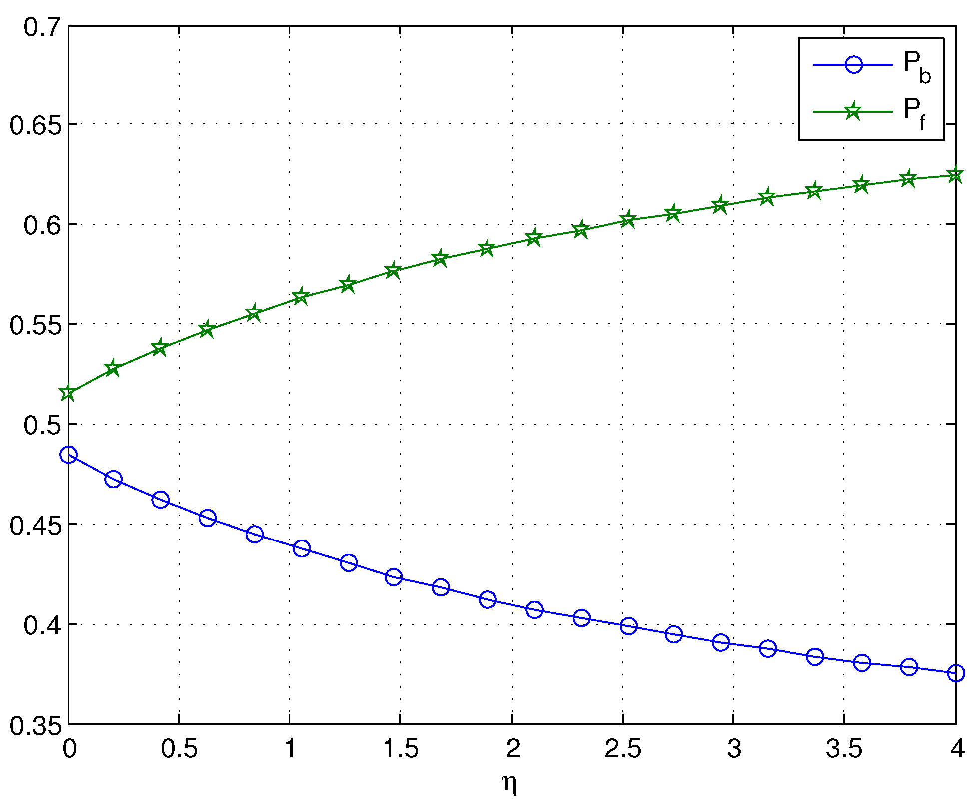
In our model, only the arrival of a negative customer can make the server break down. From Figure 1, when ${\lambda }_2$ = 0.01, we can find that $E\left[L\right]$ is almost unchanged as η increases. As expected, when ${\lambda }_2$ is not small, $E\left[L\right]$ decreases dramatically with increasing values of η. Since the service rate η is less than μ, Figure 1 indicates that $E\left[L\right]$ increases as ${\lambda }_2$ increases, and the effect of ${\lambda }_2$ on $E\left[L\right]$ is more obvious when η is smaller. In Figure 2, if we assume ${\lambda }_2$ = 0.5, it is obvious that $P_b$ decreases with increasing values of η, while $P_f$ increases as η increases. The reason is that the mean orbit length $E\left[L\right]$ and the mean service time 1/η both decrease with increasing values of η.

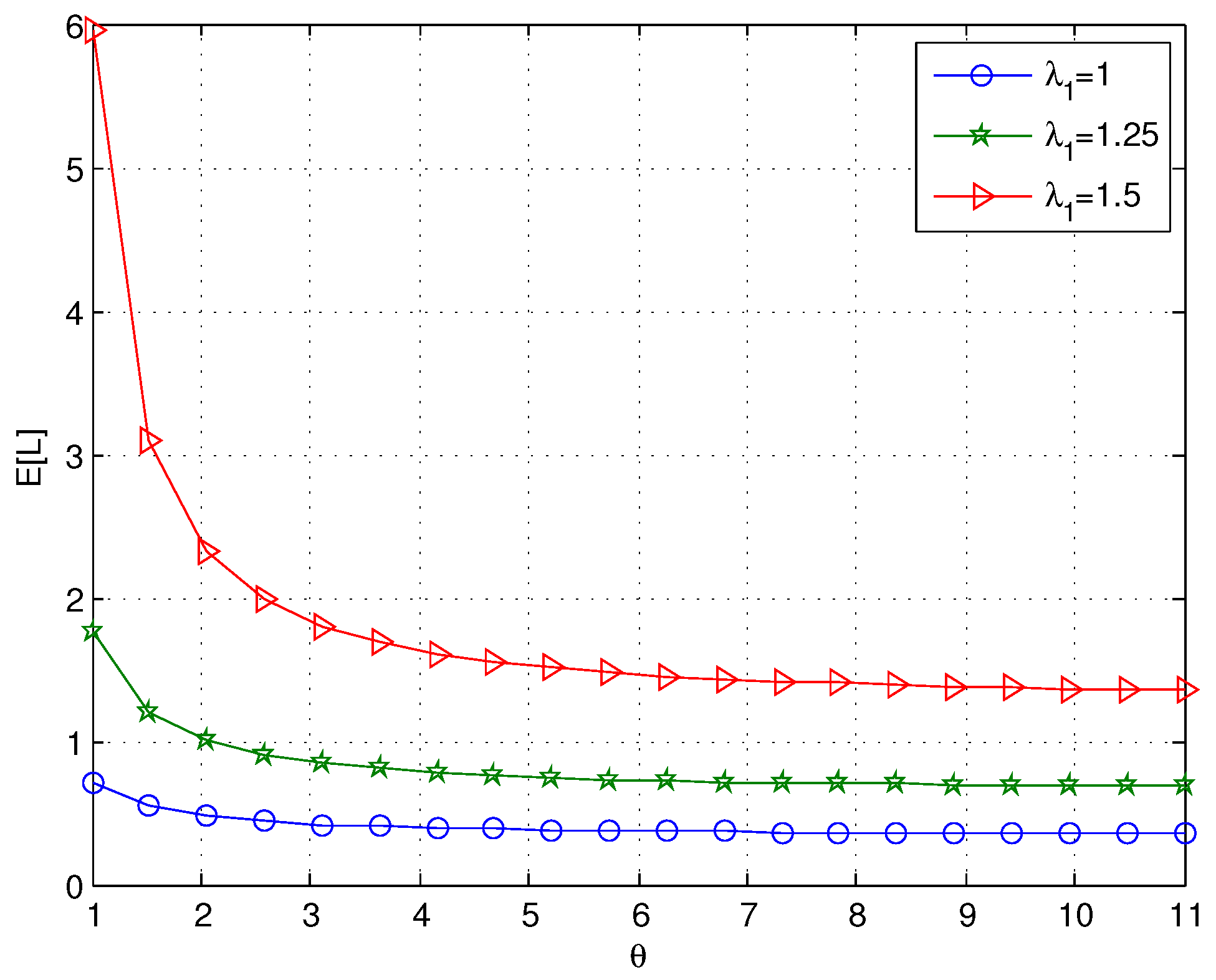
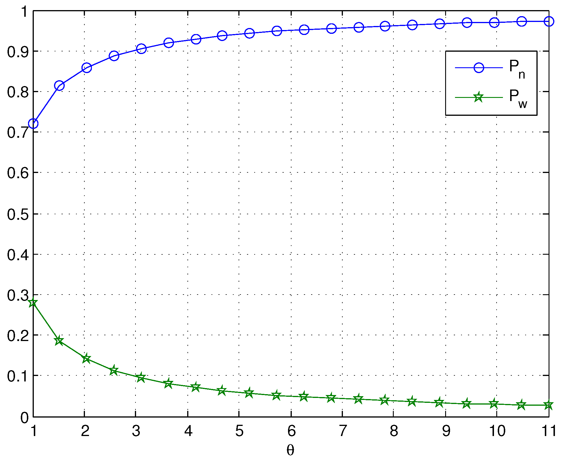
When we choose $\eta <\mu$, as shown in Figure 3 and Figure 4, $E\left[L\right]$ and $P_w$ both decrease with increasing values of θ. However, when θ is large, θ has little effect on $E\left[L\right]$ and $P_w$ as θ increases; this is because the expected working breakdown time is $1/\theta$. As expected, the probability that the server is in a normal service period approaches one for large values of θ. In Figure 3, we can see that the arrival rate ${\lambda }_1$ has a noticeable effect on $E\left[L\right]$, especially when θ is small.

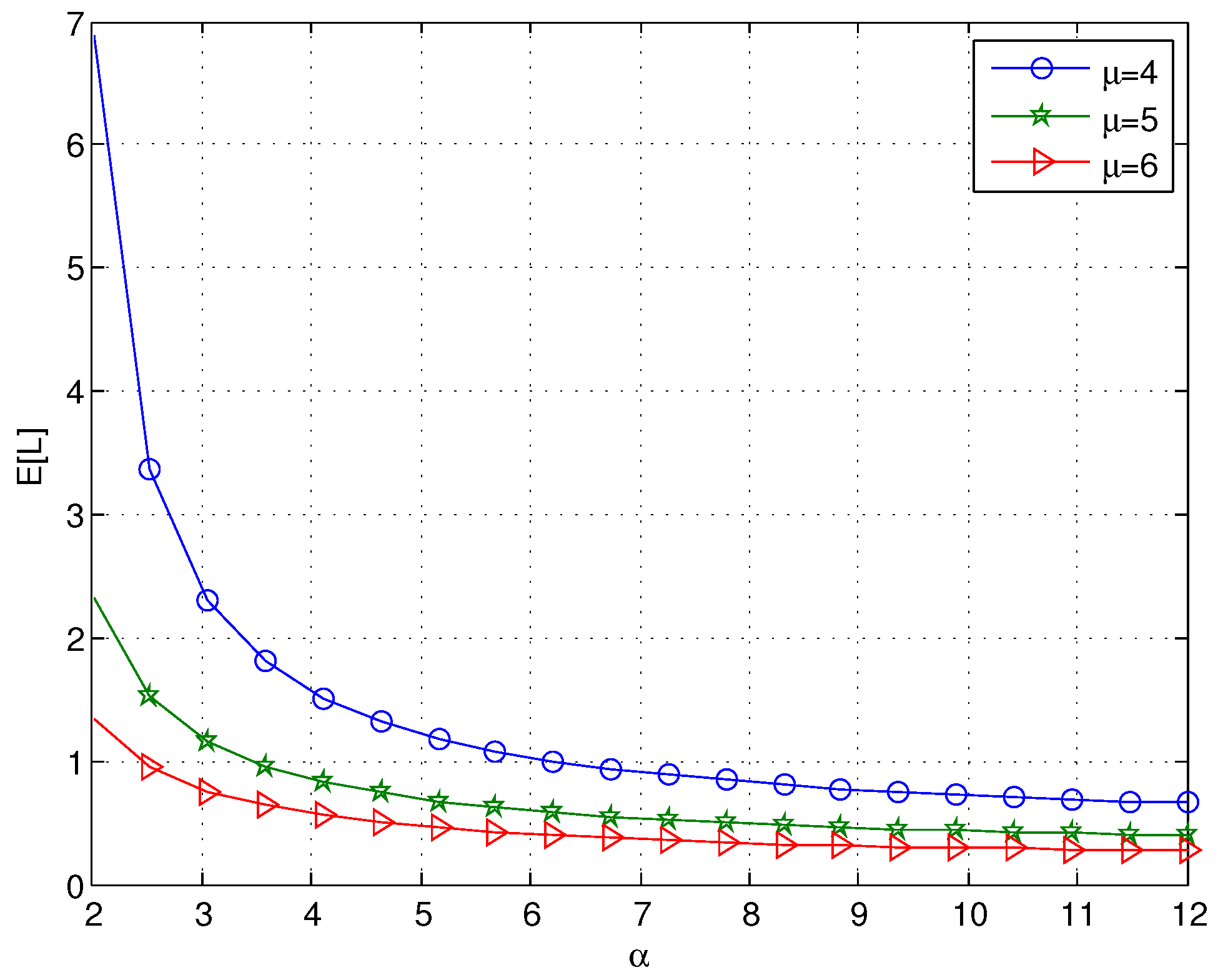
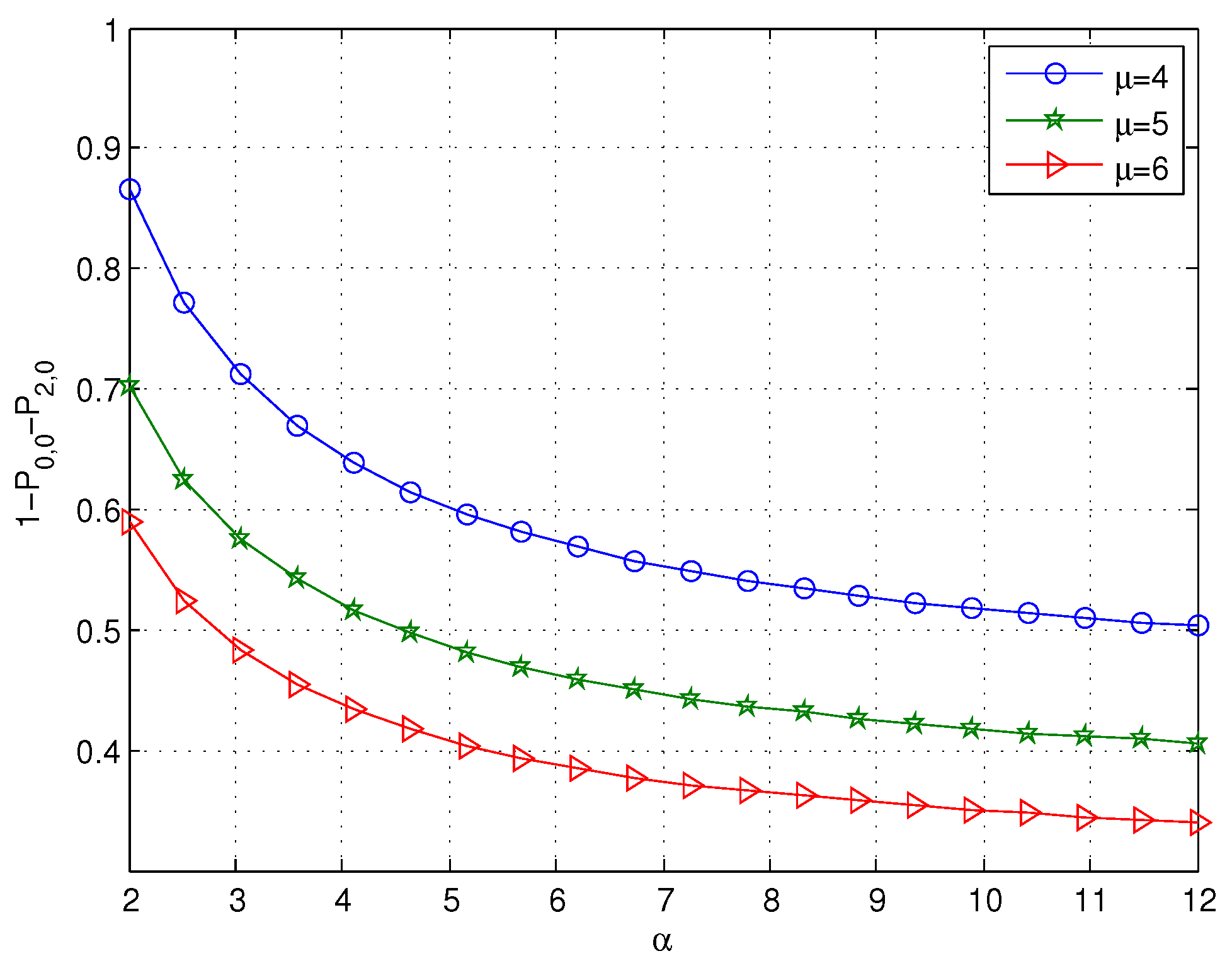
Figure 5 illustrates that $E\left[L\right]$ decreases with increasing values of α; the reason is that the mean retrial time decreases as α increases, which can decrease $E\left[L\right]$. Since the mean retrial time is $1/\alpha$, when α is large, it can be observed that the effect of α on $E\left[L\right]$ is not obvious as α increases. We can also find that $E\left[L\right]$ decreases as μ increases, which agrees with the intuitive expectation. Figure 6 reveals that the probability that the system is busy 1-$P_{0,0}$-$P_{2,0}$ decreases with increasing values of α or μ; this is because $E\left[L\right]$ decreases as α or μ increases.

5.2. Cost Analysis

In this subsection, we establish a cost function to search for the optimal service rate η, so as to minimize the expected operating cost function per unit time.

Define the following cost elements:

• $C_L$ = cost per unit time for each positive customer present in the orbit;
• $C_{\mu }$ = cost per positive customer served by the normal service rate μ;
• $C_{\eta }$ = cost per positive customer served by the lower service rate η;
• $C_{\theta }$ = fixed cost per unit time during the repair period.

Based on the definitions of each cost element listed above, the expected operating cost function per unit time can be given by:

$${\displaystyle \underset{\eta }{min}:f\left(\eta \right)=C_{L}E\left[L\right]+C_{\mu }\mu +C_{\eta }\eta +C_{\theta }\theta .}$$

Since the expected operating cost function per unit time is highly non-linear and complex, it is not easy to get the derivative of it. We assume $C_L$ = 8, $C_{\mu }$ = 20, $C_{\eta }$ = 10, $C_{\theta }$ = 6 and use the parabolic method to find the optimum value of η, say ${\eta }^{\ast }$. According to the polynomial approximation theory, the unique optimum of the quadratic function agreeing with $f\left(x\right)$ at three-point pattern $\{x_0,x_1,x_2\}$ occurs at:

$$\overline{x}=\frac{1}{2}\frac{f\left(x_0\right)(x_1^2-x_2^2)+f\left(x_1\right)(x_2^2-x_0^2)+f\left(x_2\right)(x_0^2-x_1^2)}{f\left(x_0\right)(x_1-x_2)+f\left(x_1\right)(x_2-x_0)+f\left(x_2\right)(x_0-x_1)}.$$

(26)

The parabolic method uses this approximation to improve the current three-point pattern by replacing one of its points with an approximate optimum $\overline{x}$. Then, repeating in this way isolates an optimum for $f\left(x\right)$ in an ever-narrowing range. The steps of the parabolic method can be found in [35].

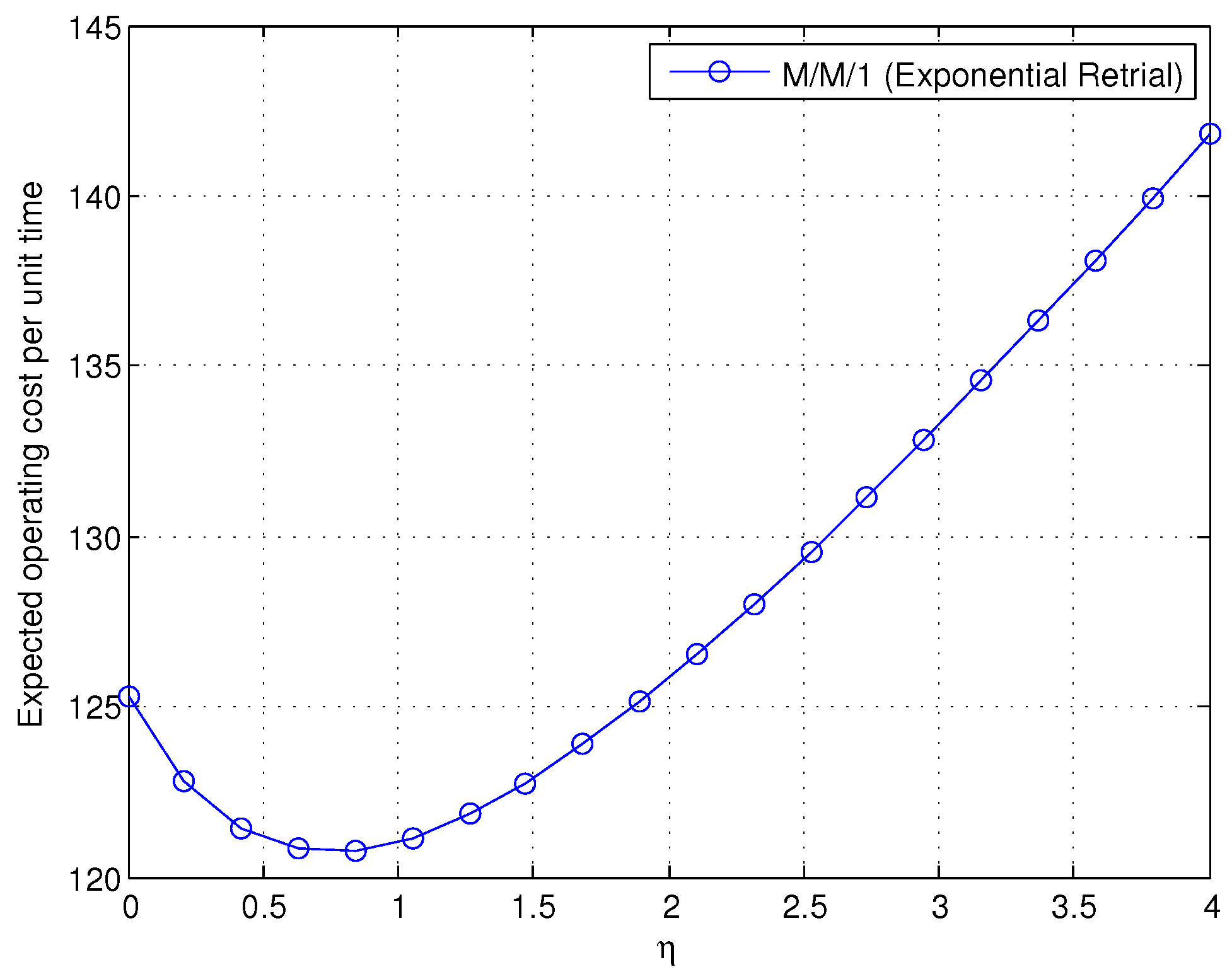
Figure 7 shows the curve of the cost function with the change of η; we can see that there is an optimal service rate η to make the cost minimized. Implementing the computer software MATLAB by the parabolic method, the error is controlled by ${10}^{-4}$. After six iterations,

Table 1. Using the parabolic method to find the optimum service rate (η) of the expected operating cost function per unit time.

No.	${\mathit{\eta }}_0$	${\mathit{\eta }}_1$	${\mathit{\eta }}_2$	$\mathit{f}\left({\mathit{\eta }}_0\right)$	$\mathit{f}\left({\mathit{\eta }}_1\right)$	$\mathit{f}\left({\mathit{\eta }}_2\right)$	$\overline{\mathit{\eta }}$	$\mathit{f}\left(\overline{\mathit{\eta }}\right)$	Tolerance
0	0.50000	$0.80000$	$1.00000$	$121.10376$	$120.74691$	121.02799	$0.76460$	120.73488	0.03540
1	0.50000	$0.76460$	$0.80000$	$121.10376$	$120.73488$	120.74691	$0.75291$	120.73370	0.01169
2	0.50000	$0.75291$	$0.76460$	$121.10376$	$120.73370$	120.73482	$0.75023$	120.73363	0.00268
3	0.50000	$0.75023$	$0.75291$	$121.10376$	$120.73363$	120.73370	$0.74938$	120.73363	0.00085
4	0.50000	$0.74938$	$0.75023$	$121.10376$	$120.73363$	120.73363	$0.74916$	120.73363	0.00021
5	0.50000	$0.74916$	$0.74938$	$121.10376$	$120.73363$	120.73363	$0.74904$	120.73363	0.00013
6	0.74904	$0.74916$	$0.74938$	$120.73363$	$120.73363$	120.73363	$0.74914$	120.73363	0.00003

shows that the minimum expected operating cost per unit time converges to the solution ${\eta }^{\ast }$ = 0.74914 with a value $f\left({\eta }^{\ast }\right)$ = 120.73363.

6. Conclusions

This paper analyzes an M/G/1 retrial G-queue with working breakdowns. During the breakdown period, the service still continues at a lower rate. Using the embedded Markov chain, we obtain the condition of stability. The supplementary variable technique is employed to discuss the probability generating function of the number of customers in the retrial orbit. Moreover, the effect of various parameters on the system performance measures are examined numerically. Under the stable condition, a cost minimization problem is considered. The novelty of this investigation is the introduction of working breakdowns to an M/G/1 retrial queue. For a future study, one can extend this model to an M${}^X$/G/1 queue.