A Comparison of Information Criteria in Clustering Based on Mixture of Multivariate Normal Distributions

Abstract

Clustering analysis based on a mixture of multivariate normal distributions is commonly used in the clustering of multidimensional data sets. Model selection is one of the most important problems in mixture cluster analysis based on the mixture of multivariate normal distributions. Model selection involves the determination of the number of components (clusters) and the selection of an appropriate covariance structure in the mixture cluster analysis. In this study, the efficiency of information criteria that are commonly used in model selection is examined. The effectiveness of information criteria has been determined according to the success in the selection of the number of components and in the selection of an appropriate covariance matrix.

1. Introduction

Models for mixtures of distributions—first discussed by Newcomb [1] and Pearson [2]—are currently very popular in clustering. Wolfe [3,4] and Day [5] proposed a multivariate normal mixture model in cluster analysis. The most important problems in clustering are choosing the number of components and identifying the structure of the covariance matrix, based on modeling with multivariate normal distributions for each component that forms the data set. Oliveira-Brochado and Martins [6] examined information criteria used in the determination of the number of components in the mixture model. Despite the many criteria used in the determination of the number of components, these criteria cannot always give accurate results. In particular, information criteria on real data sets with a known number of clusters give different results. In this study, commonly used methods for the determination of the number of clusters—Akaike Information Criterion (AIC), corrected Akaike Information Criterion (AIC_c), Bayesian Information Criterion (BIC), Classification Likelihood Criterion (CLC), Approximate Weight of Evidence Criterion (AWE), Normalized Entropy Criterion (NEC), Kullback Information Criterion (KIC), corrected Kullback Information Criterion (KIC_c), and an approximation of Kullback Information Criterion (AKIC_c) are compared according to the effectiveness of the information criteria, determined by the number of components, and determined by the success in the selection of appropriate covariance matrices and classification accuracy (CA).

2. Clustering Based on Multivariate Finite Mixture Distributions

Mixture cluster analysis based on the mixture of multivariate distributions assumes that the data to be clustered are from several subgroups or clusters, with distinct multivariate distributions. In mixture cluster analysis, each cluster is mathematically represented by a parametric distribution, such as multivariate normal distribution. The entire data set is modeled by a mixture of these distributions.

Assume that there are $n$ observations with $p$-dimensions, such that an observed random sample is expressed as $\mathit{y}={({\mathit{y}}_1^T, \dots ,{\mathit{y}}_n^T)}^T$. The probability density function of finite mixture distribution models is given by [7],

$$f({\mathit{y}}_j;\mathit{\Psi })={\displaystyle \sum }_{i=1}^g{\pi }_i{f}_i({\mathit{y}}_j;{\mathit{\theta }}_i)$$

(1)

where $f_i({\mathit{y}}_j;{\mathit{\theta }}_i)$ are probability density functions of the components and ${\pi }_i$ are the mixing proportions or weights. Here, $0\le {\pi }_i\le 1$ and ${{\displaystyle \sum }}_{i=1}^g{\pi }_i=1(i=1,\dots ,g)$. The parameter vector $\mathit{\Psi }=(\pi , \mathit{\theta })$ contains all of the parameters of the mixture models. Here $\mathit{\theta }=({\mathit{\theta }}_1,{\mathit{\theta }}_2,\dots ,{\mathit{\theta }}_g)$ denotes unknown parameters of the probability density function of the ith components (subgroup or cluster) in the mixture models. In Equation (1), the number of components or clusters is represented by $g$.

The mixture likelihood approach can be used for estimation of the parameters in the mixture models. This approach assumes that the probability function can be the sum of weighted component densities. If the mixture likelihood approach is used for clustering, the clustering problem becomes a problem of estimating the parameters of a mixture distribution model. The maximum-likelihood function is given as follows [8],

$$L_M({\mathit{\theta }}_1,{\mathit{\theta }}_2,\dots ,{\mathit{\theta }}_g;{\pi }_1,\dots ,{\pi }_g|\mathit{y})={{\displaystyle \prod }}_{j=1}^n{{\displaystyle \sum }}_{i=1}^g{\pi }_i{f}_i({\mathit{y}}_j|{\mathit{\theta }}_i)$$

(2)

The most widely used approach for parameter estimation is the Expectation-Maximization (EM) algorithm [9].

In the EM framework, the data $\mathit{y}={({\mathit{y}}_1^T,{\mathit{y}}_2^T,\dots ,{\mathit{y}}_n^T)}^T$ are considered incomplete because their associated component label vectors ${\mathit{z}}_1,{\mathit{z}}_2,\dots ,{\mathit{z}}_n$ are not observed. The component label variables $z_{ij}$ are consequently introduced, where $z_{ij}$ is defined to be one or zero, according to whether $y_j$ did or did not arise from the ith component of the mixture model ($i=1,2,\dots ,g$; $j=1,2,\dots ,n$). The completed data vector is represented as follows

$${\mathit{y}}_c={({\mathit{y}}^T,{\mathit{z}}^T)}^T$$

(3)

where

$$\mathit{z}={({\mathit{z}}_1^T,{\mathit{z}}_2^T,\dots ,{\mathbf{z}}_n^T)}^T$$

(4)

is the unobservable vector of component-indicator variables. The log-likelihood function for the completed data is shown as

$$\text{log}{L}_c(\mathit{\Psi })={{\displaystyle \sum }}_{i=1}^g{{\displaystyle \sum }}_{j=1}^n{z}_{ij}\left[\text{log}{\pi }_i+\text{log}{f}_i({\mathit{y}}_j;{\mathit{\theta }}_i)\right]$$

(5)

3. EM Algorithm

The EM algorithm is applied to this problem by treating the $z_{ij}$ as missing data. In this part, the E and M steps of the EM algorithm are described for the mixture distribution models [7].

E step: Log-likelihood function of the complete data, since $z_{ij}$ is linear in terms of its label values in the E step; given $\mathit{y}$ observed value, the instant conditional expected values of the categorical variables of ${\mathit{Z}}_{ij}$ are calculated. Here, ${\mathit{Z}}_{ij}$ is a random variable corresponding to $z_{ij}$. For parameter vector $\mathit{\Psi }$, the initial value ${\mathit{\Psi }}^{(0)}$ is assigned. In the first loop of the EM algorithm, while $\mathit{y}$ is given for the E step, the conditional expected value of $\text{log}{L}_c(\mathit{\Psi })$ is calculated with the initial value of ${\mathit{\Psi }}^{(0)}$.

$$Q(\mathit{\Psi };{\mathit{\Psi }}^{(0)})=E_{{\mathit{\Psi }}^{(0)}}\left\{\text{log}{L}_c(\mathit{\Psi })|\mathit{y}\right\}$$

(6)

In the (k + 1)th loop of the E step of the EM algorithm, the expression $Q(\mathit{\Psi };{\mathit{\Psi }}^{(k)})$ must be represented. Here, ${\mathit{\Psi }}^{(k)}$ is a value of vector $\mathit{\Psi }$ which is obtained from the kth step of EM. Since the Eth step of the (k + 1)th loop of the EM algorithm, where $i=1,2,\dots ,g$ and $j=1,2,\dots ,n$ the formula below is calculated.

$$E_{{\mathit{\Psi }}^{(k)}}(Z_{ij}|\mathit{y})=p{r}_{{\mathit{\Psi }}^{(k)}}\left\{Z_{ij}=1|\mathit{y}\right\}={\mathsf{\tau }}_i({\mathit{y}}_j;{\mathit{\Psi }}^{(k)})=\frac{{\pi }_i^{(k)}{f}_i({\mathit{y}}_j;{{\mathit{\theta }}_i}^{(k)})}{{{\displaystyle \sum }}_{m=1}^g{\pi }_m^{(k)}{f}_m({\mathit{y}}_j;{{\mathit{\theta }}_m}^{(k)})}$$

(7)

Here, the expression of ${\tau }_i({\mathit{y}}_j;{\mathit{\Psi }}^{(k)})$ is the membership probability of pattern ${\mathit{y}}_j$ in segment $i$ (posterior probability). While $\mathit{y}$ is given using the expression in Equation (7), the conditional probability in Equation (5) can be calculated as follows

$$Q(\mathit{\Psi };{\mathit{\Psi }}^{(k)})={{\displaystyle \sum }}_{i=1}^g{{\displaystyle \sum }}_{j=1}^n{\tau }_i({\mathit{y}}_j;{\mathit{\Psi }}^{(k)})\left\{\text{log}{\pi }_i+\text{log}{f}_i({\mathit{y}}_j;{\mathit{\theta }}_i)\right\}$$

(8)

M step: In the (k + 1)th loop of the EM algorithm, the estimated value ${\mathit{\Psi }}^{(k+1)}$ of $\mathit{\Psi }$, defined in parameter space $\mathit{\Omega }$, that makes the $Q(\mathit{\Psi };{\mathit{\Psi }}^{(k)})$ function maximum is calculated. In the finite mixture probability distribution model, the current estimate ${\pi }_i^{(k+1)}$ of ${\pi }_i$ is done independently from the updated vector of the unknown parameters in component density $\mathit{\xi }$.

If $z_{ij}$’s are observed, the maximum likelihood estimation of ${\pi }_i$ for completed data can be found as

$${\widehat{\pi }}_i={{\displaystyle \sum }}_{j=1}^n\frac{z_{ij}}{n}, (i=1,2,\dots ,g)$$

(9)

If the logarithm takes in completed data in the Eth step of the EM algorithm, ${\tau }_i({\mathit{y}}_j;{\mathit{\Psi }}^{(k)})$ values are used instead of the $z_{ij}$ expression. Similarly, when the current estimate ${\pi }_i^{(k+1)}$ of ${\pi }_i$ is calculated, ${\tau }_i({\mathit{y}}_j;{\mathit{\Psi }}^{(k)})$ is used instead of the $z_{ij}$ expression in Equation (9), as shown below:

$${\pi }_i^{(k+1)}={{\displaystyle \sum }}_{j=1}^n\frac{{\tau }_i({\mathit{y}}_j;{\mathit{\Psi }}^{(k)})}{n}, (i=1,2,\dots ,g)$$

(10)

In the (k + 1)th iteration of the Mth step of the EM algorithm, the current value ${\mathit{\xi }}^{(k+1)}$ of $\mathit{\xi }$ is defined as

$${{\displaystyle \sum }}_{i=1}^g{{\displaystyle \sum }}_{j=1}^n\frac{{\tau }_i({\mathit{y}}_j;{\mathit{\Psi }}^{(k)})\partial \text{log}{f}_i({\mathit{y}}_j;{\mathit{\theta }}_i)}{\partial \mathit{\xi }}=0$$

(11)

The E and M steps are repeated until the convergence criterion in the EM algorithm is satisfied. As a convenient stopping rule for convergence, if the difference of $L({\mathit{\Psi }}^{(k+1)})-L({\mathit{\Psi }}^{(k)})$ is quite small or stable, the algorithm is terminated.

4. The Mixture of Multivariate Normal Distribution

The mixture density function of the multivariate normal distribution is given by [7];

$$f({\mathit{y}}_j;\mathit{\Psi })={\displaystyle {\displaystyle \sum }_{i=1}^g}{\pi }_i{\Phi }_i({\mathit{y}}_j;{\mathit{\mu }}_i,{\mathbf{\Sigma }}_i)$$

(12)

where ${\Phi }_i({\mathit{y}}_j;{\mathit{\mu }}_i,{\mathbf{\Sigma }}_i)$ is a multivariate normal distribution function, such that

$${\Phi }_i({\mathit{y}}_j;{\mathit{\mu }}_i,{\mathbf{\Sigma }}_i)={(2\pi )}^{-\frac{p}{2}}{\left|{\Sigma }_i\right|}^{-\frac{1}{2}}{e}^{\left\{-\frac{1}{2}{({\mathit{x}}_j-{\mu }_i)}^T{\Sigma }_k^{-1}({\mathit{x}}_j-{\mu }_i)\right\}}$$

(13)

Here, the mean vector is ${\mathit{\mu }}_i$, and the covariance matrix is ${\mathbf{\Sigma }}_i$, $i=1,2,\dots ,g$, and $j=1,2,\dots ,n$. In this case, all unknown parameters of the model are shown as $\mathit{\Psi }={({\pi }_1,\dots ,{\pi }_{g-1},{\mathit{\xi }}^T)}^T$. Here, $\mathit{\xi }$ occurs from the mean compound vectors $\mathit{\mu }=({\mu }_1,{\mu }_2,\dots ,{\mu }_g)$ and the compound covariance matrix $\mathbf{\Sigma }=({\Sigma }_1,{\Sigma }_2,\dots ,{\Sigma }_g)$ of the parameters of the compound probability density function in the mixture distribution model. Posterior probability is given as

$${\tau }_i({\mathit{y}}_j;\mathit{\Psi })=\frac{{\pi }_i\Phi ({\mathit{y}}_j;{\mathit{\mu }}_i,{\mathbf{\Sigma }}_i)}{{{\displaystyle \sum }}_{h=1}^g{\pi }_i\Phi ({\mathit{y}}_j;{\mathit{\mu }}_h,{\mathbf{\Sigma }}_h)} , i=1,2,\dots ,g \text{and} j=1,2,\dots ,n$$

(14)

Maximum likelihood estimators of updated mixture proportions ${\pi }_i$, and mean vector ${\mu }_i$ of the (k + 1)th iteration of the Mth step is calculated, respectively, by

$${\pi }_i^{(k+1)}={\displaystyle {\displaystyle \sum }_{j=1}^n}\frac{{\tau }_i({\mathit{y}}_j;{\mathit{\Psi }}^{(k)})}{n}$$

(15)

$${\mathit{\mu }}_i^{(k+1)}=\frac{{{\displaystyle \sum }}_{j=1}^n{\tau }_i({\mathit{y}}_j;{\mathit{\Psi }}^{(k)}){\mathit{y}}_j}{{{\displaystyle \sum }}_{j=1}^n{\tau }_i({\mathit{y}}_j;{\mathit{\Psi }}^{(k)})}$$

(16)

Current estimates of the covariance matrix (${\Sigma }_i$) of the component probability density are calculated via the following formula

$${\mathbf{\Sigma }}_i^{(k+1)}=\frac{{{\displaystyle \sum }}_{j=1}^n{\mathsf{\tau }}_i({\mathit{y}}_j;{\mathit{\Psi }}^{(k)})({\mathit{y}}_j-{\mathit{\mu }}_i^{(k+1)}){({\mathit{y}}_j-{\mathit{\mu }}_i^{(k+1)})}^T}{{{\displaystyle \sum }}_{j=1}^n{\tau }_i({\mathit{y}}_j;{\mathit{\Psi }}^{(k)})} , (i=1,2,\dots ,g)$$

(17)

5. Information Criteria for Model Selection in Model Based Clustering

Model selection is one of the most important problems in mixture cluster analysis based on the mixture of multivariate normal distributions. Model selection includes the determination of the number of components (cluster) and the selection of an appropriate covariance structure in the mixture cluster analysis. Information criteria are often used in the model selection in mixture cluster analysis. In the literature, information criteria are usually computed as twice a negative value of the bias correction

$$-2\text{log}L(\widehat{\mathit{\Psi }})+2C$$

(18)

Here, the first term represents the lack of harmonization, and the second term $C$ is a measure of complexity. $C$ is usually called the penalty term. The best model that makes the term $-2\text{log}L(\widehat{\mathit{\Psi }})+2C$ minimum is selected. Some commonly used information criteria in the literature are given below [6,7,10]:

• If the number of parameters in the model is shown by $d$, this is called as Akaike’s Information Criterion (AIC), defined as

  $$\text{AIC}=-2\text{log}L(\widehat{\mathit{\Psi }})+2d$$

  (19)

  A model that makes the AIC score minimum can be selected as the best model [11].
• When d is large relative to the sample size n (which includes when n is small, for any d) there is a small-sample version called AIC_c. AIC_c is defined as

  $${\text{AIC}}_{\mathrm{c}}=-2\text{log}L(\widehat{\mathit{\Psi }})+2dn/(n-d-1)$$

  (20)

  The model that yields the minimum AIC_c score can be selected as the best model [12].
• If we take the number of parameters in the mixture distribution models $d$, and the number of observations $n$, the Bayesian Information Criterion (BIC) can be calculated as

  $$\text{BIC}=-2\text{log}L(\widehat{\mathit{\Psi }})+d\text{log}(n)$$

  (21)

  The model that gives the minimum BIC score can be selected as the best model [13].
• The Hathaway [14] mixture logarithmic likelihood is formulated as

  $$\text{log}L(\mathit{\Psi })=\text{log}{L}_c(\mathit{\Psi })-EN(\tau )$$

  (22)

  Here, Equation (23) is defined as

  $$EN(\tau )=-{{\displaystyle \sum }}_{i=1}^g{{\displaystyle \sum }}_{j=1}^n{\tau }_{ij}\text{log}{\tau }_{ij}$$

  (23)

  where $-EN(\tau )$ is the entropy of the fuzzy classification matrix $C=\left\{({\tau }_{ij})\right\}$.
  The CLC (Classification Likelihood Criterion) is defined as

  $$\text{CLC}=-2\text{log}L(\widehat{\mathit{\Psi }})+2EN(\widehat{\tau })$$

  (24)

  A model that gives the minimum CLC score can be selected as the best model [15].
• The Approximate Weight of Evidence (AWE) is expressed as

  $$\text{AWE}=-2\text{log}{L}_c+2d(3/2+\text{log}n)$$

  (25)

  A model that gives the minimum AWE score can be selected as the best model [16].
• The Normalized Entropy Criterion (NEC) is shown as below [17]

  $${\text{NEC}}_{\mathrm{g}}=\frac{EN(\widehat{\tau })}{\text{log}L(\widehat{\mathit{\Psi }})-\text{log}L({\widehat{\mathit{\Psi }}}^{*})}$$

  (26)

  Here, ${\widehat{\mathit{\Psi }}}^{*}$is a maximum likelihood estimator for $\mathit{\Psi }$ when (g = 1). The minimum NEC for the number of components $g$ is selected as the number of clusters. When $g=1$, entropy takes the value of zero. For this case, Biernacki et al. [18] suggested the selection of the minimum value of NEC where the number of components $g>1$, including NEC < 1.
• Cavanaugh [19] has proposed an asymptotic unbiased estimator of the Kullback information criterion (KIC). KIC is defined as

  $$\text{KIC}=-2\text{log}L(\widehat{\mathit{\Psi }})+3(d+1)$$

  (27)
• Bias correction of the Kullback information criterion (KIC_c) and an approximation of the Kullback information criterion (AKIC_c) are shown as below [20,21]

  $${\text{KIC}}_{\mathrm{c}}=-2\text{log}L(\widehat{\mathit{\Psi }})+\frac{2(d+1)n}{n-d-2}-n\psi (\frac{n-d}{2})+n\text{log}(\frac{n}{2})$$

  (28)

  $${\text{AKIC}}_{\mathrm{c}}=-2\text{log}L(\widehat{\mathit{\Psi }})+\frac{(d+1)(3n-d-2)}{n-d-2}+\frac{d}{n-d}$$

  (29)

  Here, $d$ is the number of parameters in the model, $n$ is the sample size, and $\psi$(.) is the digamma or the psi function.

6. Application and Results

In this section, the performances of the information criteria used for the determination of the number of clusters are compared. Moreover, the efficiency of the different types of covariance matrices are investigated in the model based on clustering. The comparison of the information criteria is performed using two different settings. First, commonly used real data sets are used. Second, synthetic data sets are generated by using the properties of these real data sets, and they are used for comparison.

The properties of real data sets are given in

Table 1. Descriptions of real data sets.

Data Sets *	Sample Size ($\mathit{n}$)	Number of Variables ($\mathit{p}$)	Number of Clusters ($\mathit{g}$)
Liver Disorders	345	6	2
Iris	150	4	3
Wine	178	13	3
Ruspini	75	2	4
Vehicle Silhouettes	846	18	4
Landsat Satellite	6435	36	6
Image Segmentation	2310	19	7

Note: * Data sets are taken from the website of UCI Machine Learning Repository [22].

. Moreover, the computed information criteria for each different data set are provided in

Table 2. Information criteria results in the determination of the number of clusters for the Liver Disorders data set.

Liver Disorders Data Set
$\mathit{g}$	2 *	3	4	5
AIC	14,752.43	14,693.75	14,605.72 *	14,643.68
AICc	14,773.75	14,747.17	14,712.44 *	14,833.53
AKICc	14,832.79	14,834.99	14,829.30 *	14,979.88
AWE	15,503.68 *	15,865.24	16,176.27	16,582.91
BIC	14,963.83 *	15,012.76	15,032.36	15,177.93
CLC	14,695.89	14,646.21	14,546.00	14,541.41 *
KIC	14,810.43	14,779.75	14,719.72 *	14,785.68
KICc	14,837.70 *	14,846.93	14,852.24	15,018.79
NEC	0.06956 *	0.13412	0.15797	0.16811

Note: * True value of $g$ or value of $g$ given by criterion. AIC: Akaike information criterion; AIC_c: corrected Akaike information criterion; AKIC_c: approximation of Kullback information criterion; AWE: approximate weight of evidence criterion; BIC: Bayesian information criterion; CLC: classification likelihood criterion; KIC: Kullback information criterion; KIC_c: corrected Kullback information criterion; NEC: normalized entropy criterion.

,

Table 3. Information criteria results in the determination of the number of clusters for the Iris data set.

Iris Data Set
$\mathit{g}$	2	3 *	4	5
AIC	487.11	449.15	448.86 *	474.12
AICc	501.61	486.86 *	527.53	622.12
AKICc	534.98 *	536.37	593.75	706.14
AWE	806.74 *	944.15	1126.55	1378.81
BIC	574.42 *	581.61	626.49	696.90
CLC	429.12	371.21	358.29 *	415.24
KIC	519.11	496.15 *	510.86	551.12
KICc	538.21 *	544.45	609.73	734.14
NEC	0.00003 *	0.02524	0.06393	0.20542

Note: * True value of $g$ or value of $g$ given by criterion.

,

Table 4. Information criteria results in the determination of the number of clusters for the Wine data set.

Wine Data Set
$\mathit{g}$	2	3 *	4	5
AIC	6446.14	6255.42 *	6258.49	6382.48
AICc	3703.01 *	4811.48	4804.11	4796.89
AKICc	3965.94 *	5127.50	5223.44	5320.90
AWE	8821.75 *	9827.04	11,021.22	12,345.63
BIC	7111.13 *	7254.50	7591.66	8049.74
CLC	6028.77	5630.88	5421.88	5343.12 *
KIC	6658.14	6572.42*	6680.49	6909.48
KICc	-	-	-	-
NEC	0.00099 *	0.00334	0.00112	0.00650

Note: * True value of $g$ or value of $g$ given by criterion. KIC_c could not be calculated because $d$ is greater than $n$.

,

Table 5. Information criteria results in the determination of the number of clusters for the Ruspini data set.

Ruspini Data Set
$\mathit{g}$	2	3	4 *	5
AIC	1409.23	1369.92	1329.89	1322.48 *
AICc	1413.42	1380.66	1351.54 *	1361.15
AKICc	1428.43	1402.43	1380.33 *	1397.39
AWE	1515.21 *	1534.05	1552.26	1602.17
BIC	1434.72	1409.32	1383.19 *	1389.69
CLC	1387.23	1336.26	1284.66	1264.76 *
KIC	1423.23	1389.92	1355.89	1354.48 *
KICc	1429.34	1404.71	1384.81 *	1405.06
NEC	0.00001 *	0.00184	0.00328	0.00108

Note: * True value of $g$ or value of $g$ given by criterion.

,

Table 6. Information criteria results in the determination of the number of clusters for the Vehicle Silhouettes data set.

Vehicle Silhouettes Data Set
$\mathit{g}$	2	3	4 *	5
AIC	80,747.84	78,171.46	76,987.29 *	77,496.43
AICc	81,365.96	80,521.67	90,402.17	60,158.93 *
AKICc	81,753.37	81,112.56	91,366.48	61,230.64 *
AWE	86,249.13 *	86,431.40	88,003.06	91,282.76
BIC	82,544.50	80,868.81	80,585.34 *	81,995.18
CLC	80,002.82	77,053.69	75,493.95 *	75,642.25
KIC	81,129.84	78,743.46	77,749.29 *	78,448.43
KICc	81,877.05	81,488.13 *	92,531.84	-
NEC	0.00204 *	0.00217	0.00227	0.00408

Note: * True value of $g$ or value of $g$ given by criterion. KIC_c ($g=5$) could not be calculated because $d$ is greater than $n$.

,

Table 7. Information criteria results in the determination of the number of clusters for the Landsat Satellite data set.

Landsat Satellite Data Set
$\mathit{g}$	5	6 *	7	8
AIC	1,255,771.79	1,251,929.66 *	1,253,394.33	1,252,217.99
AICc	1,264,231.87 *	1,267,975.95	1,285,377.58	1,330,205.05
AKICc	1,267,757.79 *	1,272,212.70	1,290,337.97	1,335,962.02
AWE	1,321,382.18	1,330,827.27	1,345,663.27	1,357,765.53
BIC	1,279,559.84 *	1,280,476.68	1,286,700.30	1,290,282.93
CLC	1,249,208.09	1,244,214.25	1,244,611.32	1,242,274.65 *
KIC	1,259,288.79	1,256,149.66 *	1,258,317.33	1,257,843.99
KICc	1,269,326.31 *	1,274,849.92	1,294,725.15	1,343,659.52
NEC	0.00447	0.00659	0.00969	0.01167

Note: * True value of $g$ or value of $g$ given by criterion. AWE and NEC have found $g=2$.

and

Table 8. Information criteria results in the determination of the number of clusters for the Image Segmentation data set.

Image Segmentation Data Set
$\mathit{g}$	5	6	7 *	8
AIC	67,666.74	64,307.94	59,502.75 *	61,395.91
AICc	68,423.32	65,517.43	61,352.58 *	64,152.73
AKICc	69,193.28	66,441.60	62,431.40 *	65,386.90
AWE	80,315.60	79,480.18	77,188.94 *	81,663.54
BIC	72,055.92	69,576.11	65,649.90 *	68,422.05
CLC	66,189.23	62,524.84	57,404.63 *	59,050.26
KIC	68,433.74	65,227.94	60,575.75 *	62,621.91
KICc	69,356.93	66,692.97	62,798.53 *	65,905.24
NEC	0.00066	0.00063	0.00049 *	0.00119

Note: * True value of $g$ or value of $g$ given by criterion.

.

The appropriate number of clusters is determined as the value which gives the minimum information criteria. According to Table 2, the number of clusters of the Liver Disorders data set is correctly determined via AWE, BIC, KIC_c, and NEC. In Table 3, AIC_c and KIC could accurately determine the number of clusters of the Iris data set. The number of clusters of the Wine data set is correctly determined via AIC and KIC in Table 4.

According to Table 5, the number of clusters of the Ruspini [23] data set is correctly determined via AIC_c, AKIC_c, BIC, and KIC_c. In Table 6, the number of clusters of the Vehicle Silhouettes data set is correctly determined by AIC, BIC, CLC, and KIC.

According to Table 7, the number of clusters for the Landsat Satellite data set is correctly determined via AIC and KIC. In Table 8, the number of clusters for the Image Segmentation data set is correctly determined by all information criteria.

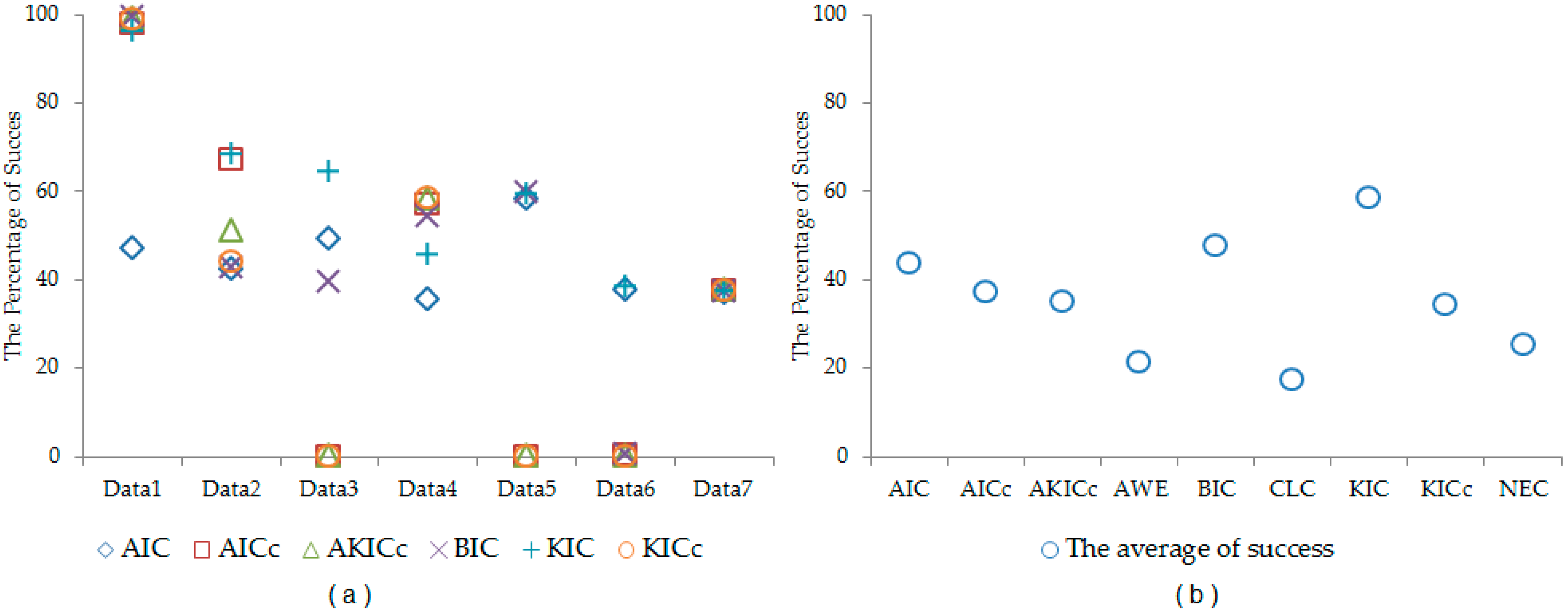
In Table 2, Table 3, Table 4, Table 5, Table 6, Table 7 and Table 8, the performance of each information criterion varies in each data set. In order to make general conclusions, a simulation study is provided. By using the properties of each real data set, synthetic data sets are generated. In this simulation, we generated 1000 data sets according to each real data set. The synthetic data sets are generated from Liver, Iris, Wine, Ruspini, Vehicle, Landsat, and Image data sets. The cluster number determination accuracy is computed for each information criterion. The results are given in

Table 9. The accuracy of determining the cluster numbers from the information criteria according to synthetic data sets.

Synthetic Data Sets	AIC	AICc	AKICc	AWE	BIC	CLC	KIC	KICc	NEC
Data1 (Generated from Liver)	46.8	97.9	98.9	98.6	99.1	52.5	95.8	98.9	91.3
Data2 (Generated from Iris)	42	66.9	50.9	1.4	42.4	4.7	68.3	44.1	2.3
Data3 (Generated from Wine)	48.9	0	0	0	39.1	0.8	64	0	34.1
Data4 (Generated from Ruspini)	35.4	56.8	58.1	13.4	54	21.7	45.4	58.4	19.3
Data5 (Generated from Vehicle)	58	0	0	3.2	59.6	12	59	0	18.3
Data6 (Generated from Landsat)	37.6	0.1	0	0	0.3	2.4	38	0	0.1
Data7 (Generated from Image)	36.6	37.3	37.5	32.1	37.2	26.7	37	37.3	9.5
The average of success	43.6	37	35.1	21.2	47.4	17.3	58.2	34.1	25

Note: The best performance is indicated in bold.

and Figure 1. According to simulation results, better results are obtained by using KIC.

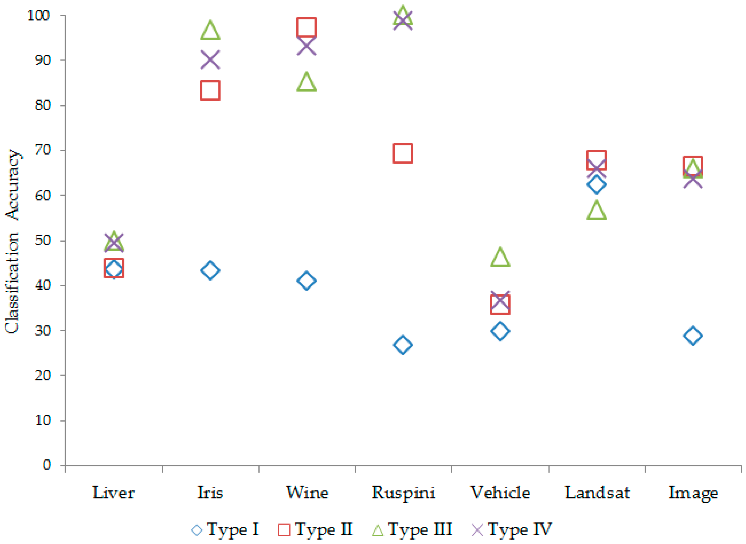
The efficiency of different types of covariance structures in mixture clustering based on a mixture of multivariate normal distributions is investigated.

According to the number of clusters regarding each data set, classification accuracy and information criteria are computed for each covariance structure. The results are given in

Table 10. Classification accuracy (CA) and information criteria results for real data sets, according to different types of covariance structures.

Data Sets	Covariance Types	CA	AIC	AICc	AKICc	BIC	KIC	KICc
Liver Disorders	I	43.48	15,371.1	15,378.8	15,416.4	15,501.8	15,408.1	15,418.2
	II	43.77	15,605.7	15,608.1	15,630.4	15,678.7	15,627.7	15,630.9
	III	49.86	14,752.4	14,773.7	14,832.8	14,963.8	14,810.4	14,837.7
	IV	49.28	14,905.2	14,909.3	14,937.7	15,001.3	14,933.2	14,938.6
Iris	I	43.33	799.5	809.1	837.1	871.7	826.5	839.3
	II	83.33	1326.9	1332.1	1353.9	1381.1	1347.9	1355.1
	III	96.67	449.1	486.9	536.4	581.6	496.1	544.5
	IV	90.00	666.5	677.9	708.1	744.8	695.5	710.7
Wine	I	41.01	6851.2	7631.5	7799.2	7271.2	6986.2	7908.1
	II	97.19	7528.8	7662.4	7751.0	7783.3	7611.8	7777.2
	III	85.39	6255.4	4811.5	5127.5	7254.5	6572.4	4864.0
	IV	93.26	6757.1	6890.7	6979.3	7011.7	6840.1	7005.6
Ruspini	I	26.67	1546.8	1553.8	1572.2	1579.3	1563.8	1573.7
	II	69.33	1545.0	1551.0	1568.2	1575.1	1561.0	1569.5
	III	100.00	1329.9	1351.5	1380.3	1383.2	1355.9	1384.8
	IV	98.67	1324.2	1338.0	1362.1	1368.2	1346.2	1365.0
Vehicle Silhouettes	I	29.79	85,618.6	85,821.4	86,072.8	86,784.7	85,867.6	86,117.5
	II	35.70	111,399.9	111,423.2	111,519.8	111,840.8	111,495.9	111,525.4
	III	46.45	76,987.3	90,402.2	91,366.5	80,585.3	77,749.3	92,531.8
	IV	36.64	102,899.9	102,962.3	103,113.4	103,596.8	103,049.9	103,127.9
Landsat Satellite	I	62.46	1,349,241.4	1,349,525.3	1,350,416.2	1,355,245.9	1,350,131.4	1,350,483.6
	II	67.69	1,828,135.0	1,828,156.5	1,828,416.7	1,829,874.8	1,828,395.0	1,828,422.0
	III	56.67	1,251,929.7	1,267,975.9	1,272,212.7	1,280,476.7	1,256,149.7	1,274,849.9
	IV	65.87	1,618,062.2	1,618,126.1	1,618,566.4	1,621,020.5	1,618,502.2	1,618,582.0
Image Segmentation	I	28.70	38,937.2	39,000.2	39,257.9	40,396.4	39,194.2	39,273.0
	II	66.54	286,194.3	286,210.9	286,348.3	286,964.1	286,331.3	286,352.3
	III	65.93	59,502.7	61,352.6	62,431.4	65,649.9	60,575.7	62,798.5
	IV	63.68	198,790.6	198,841.7	199,075.3	200,111.9	199,023.6	199,087.5
Type I $(\mathbf{\Sigma })$: Covariance matrix of the data set used for clustering.
Type II $({\mathit{\sigma }}_{\mathit{i}}^{\mathbf{2}}\mathit{I})$: Variance matrix of the data set used for clustering.
Type III $({\mathbf{\Sigma }}_{\mathit{k}})$: Covariance matrix of each subgroup in the data set.
Type IV $({\mathit{\sigma }}_{\mathit{i}\mathit{k}}^{\mathbf{2}}\mathit{I})$: Variance matrix of each subgroup in the data set.

Note: The best performances are indicated in bold.

.

According to Table 10, the Type III $({\Sigma }_{\mathrm{k}})$ covariance matrix of each subgroup has generally performed better in the results, both in terms of the correct classification and the minimum information criteria value. The classification accuracy in mixture clustering based on a mixture of multivariate normal distributions according to covariance types is given in Figure 2.

7. Conclusions

In this study, we compared the effectiveness of information criteria in clustering analysis based on the mixture of multivariate normal distributions. As a result of this simulation study, KIC gave better results than other information criteria in the determination of the number of clusters in mixture clustering based on a mixture of multivariate normal distributions. Also, the efficiency of different types of covariance matrices are investigated in the model based clustering. The better results are obtained by the using covariance matrix of each subgroup (Type III) in mixture clustering based on a mixture of multivariate normal distributions.