Predictive Abilities of Bayesian Regularization and Levenberg–Marquardt Algorithms in Artificial Neural Networks: A Comparative Empirical Study on Social Data

Abstract

The objective of this study is to compare the predictive ability of Bayesian regularization with Levenberg–Marquardt Artificial Neural Networks. To examine the best architecture of neural networks, the model was tested with one-, two-, three-, four-, and five-neuron architectures, respectively. MATLAB (2011a) was used for analyzing the Bayesian regularization and Levenberg–Marquardt learning algorithms. It is concluded that the Bayesian regularization training algorithm shows better performance than the Levenberg–Marquardt algorithm. The advantage of a Bayesian regularization artificial neural network is its ability to reveal potentially complex relationships, meaning it can be used in quantitative studies to provide a robust model.

1. Introduction

Defining a highly accurate model for quantitative studies depends on conditions such as the distribution of variables, the number of predictors, and the complexity of interactions between variables. Preventing the model from defining a bias and choosing a statistical method that is robust and can solve complex relationships are also crucial. An Artificial Neural Network (ANN) is a popular statistical method which can explore the relationships between variables with high accuracy [1,2,3,4]. Essentially, the structure of an ANN is computer-based and consists of several simple processing elements operating in parallel [3,5,6].

An ANN consists of three layers: input, hidden, and output layers, hence it is referred to as a three-layer network. The input layer contains independent variables that are connected to the hidden layer for processing. The hidden layer contains activation functions and it calculates the weights of the variables in order to explore the effects of predictors upon the target (dependent) variables. In the output layer, the prediction or classification process is ended and the results are presented with a small estimation error [7,8].

In general, a backpropagation algorithm trains a feedforward network. In the training process, the backpropagation algorithm learns associations between a specified set of input-output pairs [9]. The backpropagation training algorithm acts as follows [7]: first, it propagates the input values forward to a hidden layer, and then, it propagates the sensitivities back in order to make the error smaller; at the end of the process, it updates the weights. The mathematical frame of the backpropagation algorithm can be seen in several studies such as “Training Feedforward Networks with the Marquardt Algorithm” by [7]. Due to the limited word count, not all of the backpropagation algorithm is presented but it can be seen in other studies.

In ANNs, some regularization techniques are used with the backpropagation training algorithm to obtain a small error. This causes the network response to be smoother and less likely to overfit to training patterns [8,10]. However, the backpropagation algorithm is slow to converge and may cause an overfitting problem. Backpropagation algorithms that can converge faster have been developed to overcome the convergence issue. Similarly, some regularization methods have been developed to solve the overfitting problem in ANNs. Among regularization techniques, Levenberg–Marquardt (LM) and Bayesian regularization (BR) are able to obtain lower mean squared errors than any other algorithms for functioning approximation problems [11]. LM was especially developed for faster convergence in backpropagation algorithms. Essentially, BR has an objective function that includes a residual sum of squares and the sum of squared weights to minimize estimation errors and to achieve a good generalized model [3,12,13,14,15].

Basically, Multilayer Perceptron Artificial Neural Network (MLPANN) or Radial Basis Function Artificial Neural Network (RBFANN) algorithms could be examined instead of BR or LM. However, it’s known that BR and LM have better performance than the conventional methods (MLPANN, RBFANN) in terms of both speed and the overfitting problem; as such, the aim was to explain BR and LM algorithms for their use with social data and compare these algorithms in terms of their predictive abilities. There are too few studies using an Artificial Neural Network with social data. It should be considered that “linear-non-linear relationship” or “data type” varies from case to case. While any architecture of neural network explains the model with small error or high accuracy for continuous variable (natural-metric data such as weight, age, amount of electric consume, temperature, humidity, etc.), maybe this architecture is not capable of explaining the model well for a non-linear relation or non-continuous data. As it is seen that the study contains a lot of nominal and ordinal variables (non-continuous), it is worth studying some artificial neural networks on social data due to different behavior of distribution.

In this study, the training algorithms of BR and LM are compared in terms of predictive ability. To compare their respective performances, the correlation coefficient between real and predicted data is compared via BR and LM for performance criteria, along with the sum of squared errors, which can also be a network performance indicator.

2. Material and Methods

2.1. Data Set (Material)

The data set was composed of 2247 university students. There are 25 variables (24 predictors and one response) in the model. The score of the target (dependent) variable was obtained from a reflective thinking scale. This is composed of 16 items and each item is measured by using a five-level Likert scale (1: Strongly disagree; 2: Disagree; 3: Uncertain; 4: Agree; 5: Strongly agree). The aim of the reflective thinking scale is to measure students’ reflective thinking levels and the score varies between 16 and 80. The reliability of reflective thinking was examined with Cronbach’s Alpha, and scored 0.792. This value shows that the reliability level of the reflective thinking scale is good. The validity of the scale was examined with principle component analysis (exploratory factor analysis) and the result of this analysis was within an acceptable boundary.

In this study, 24 predictors given to the students via a prepared questionnaire were used. Some of predictors were nominal (dichotomous or multinomial), some of them were ordinal, and the rest were continuous variables. The predictors in the model were: “1—faculty (Education, Science, Engineering, Divinity, Economics, Health)”, “2—gender”, “3—faculty department”, “4—the graduation of the branch from high school (social, science, linguistics, etc.)”, “5—class in department (1/2/3/4)”, “6—the preferred department order given at the University Entrance Examination”, “7—current transcript score”, “8—completed preschool education (yes or no)”, “9—school type graduation (science, social, divinity, vocational, etc.)”, “10—location when growing up (village, city, small town)”, “11—degree of mother’s education (primary, middle, high school, university, etc.)”, “12—degree of father’s education (primary, middle, high school, university, etc.)”, “13—monthly income of student’s family”, “14—level of satisfaction with the department”, “15—frequency of reading a newspaper”, “16—newspaper sections read”, “17—number of books read”, “18—types of book read (novel, psychological, science fiction, politic, adventure, etc.”, “19—consultation with environment (friends, etc.) on any argument (always/generally/sometimes/never)”, “20—taking notes during lesson regularly”, “21—discussion with environment (such as friend, roommate) on any issue (always/generally/sometimes/never)”, “22—any scientific research carried out yet (yes/no)”, “23—expected lesson’s details just from teacher (yes/no)”, “24—research anxiety score” (this score was taken from the Research Anxiety Scale composed of 12 items). During analysis, the independent variables are coded from 1 to 24 in order to build readable tables.

2.2. Methods

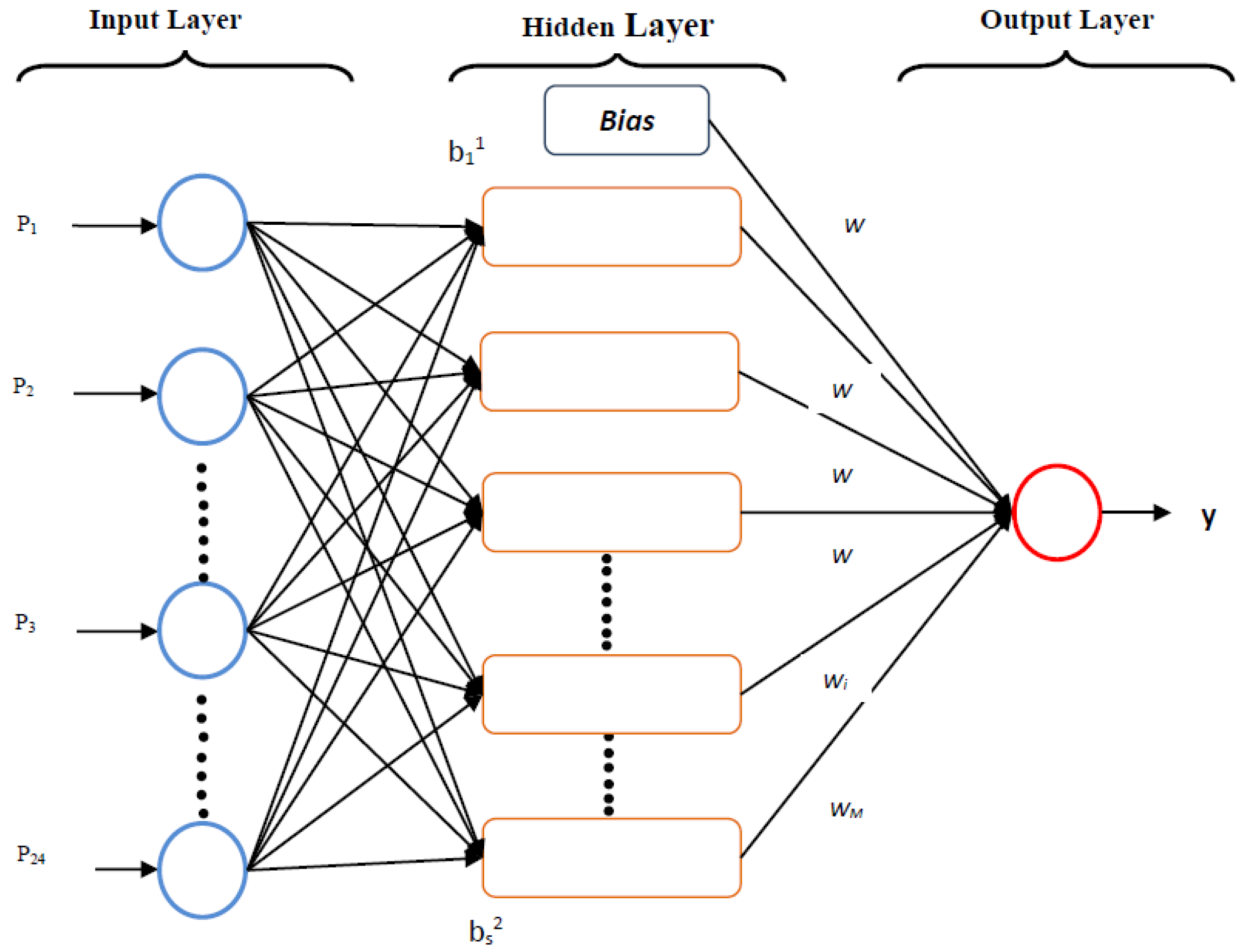
2.2.1. Feed-Forward Neural Networks with Backpropagation Algorithm

In feed-forward neural networks, otherwise known as multilayer perceptrons, the input vector of independent variables p_i is related to the target t_i (reflective thinking score) using the architecture depicted in Figure 1. This figure shows one of the commonly used networks, namely, the layered feed-forward neural network with one hidden layer. Here each single neuron is connected to those of a previous layer through adaptable synaptic weights [3,16]. Knowledge is usually stored as a set of connection weights. Training is the process of modifying the network using a learning mode in which an input is presented to the network along with the desired output, and then, the weights are adjusted so that the network attempts to produce the desired output. The weights after training contain meaningful information, whereas before training they are random and have no meaning [17].

The architecture of the network examined in the study was such that $p_i^{\prime }$ = (p_i1, p_i2, …, p_i24) contained values for 24 input (independent) variables from individual i. The input variables are associated with each of N neurons in a hidden layer by using weights (w_kj, k = 1, 2, …, N) which are specific to each independent variable (j) to neuron (k) connection. Following Mackay (2008) [18], the mapping has two forms for the relationship between output $\widehat{t}$ and independent variables:

$$\mathrm{HiddenLayer}{n}_k^{(1)}={\mathsf{\Sigma }}_{j=1}^R{w}_{kj}^{(1)}{p}_j+b_k^{(1)};\hspace{1em}{a}_k^1=f_{level-one}\left(n_k^{(1)}\right)$$

(1)

$$\mathrm{OutputLayer}{n}_k^{(2)}={\mathsf{\Sigma }}_{j=1}^{}{w}_k^{(2,1)}{a}_k^1+b_1^{(2)};\hspace{1em}{\widehat{t}}_i=a_k^{(2)}=f_{level-two}\left(n_k^{(2)}\right)$$

(2)

In the case of N neurons in the neural network, the biases are $b_1^{(1)},b_2^{(1)}\mathrm{........}{b}_N^{(1)}$. Prior to activation, the input value for neuron k is $b_k^{(1)}+{\displaystyle \sum _{j=1}^{24}{w}_{kj}{p}_j}$. Then an activation function f(.) (linear or nonlinear) is applied to the input in each neuron and v is transformed as $f_k\left(b_k^{(1)}+{\displaystyle \sum _{j=1}^{24}{w}_{kj}{p}_j}\right)$ = $f_k\left(n_k^{(1)}\right)$, k = 1, 2, ..., N. After applying activation, the activated quantity is then transferred to the output layer and gathered as ${\displaystyle \sum _{ki=1}^N{w}_k^{\prime }{f}_k\left(b_k^{(1)}+{\displaystyle \sum _{j=1}^{24}{w}_{kj}{p}_j}\right)+b^{(2)}}$, where w_k (k = 1, 2, …, N) are b₍₁₎ and b₍₂₎ bias parameters in the hidden and output layers. At the end of the process, this activated quantity is carried out again with function g(.) as $g\left[{\displaystyle \sum _{k=1}^N{w}_k^{\prime }{f}_k(.)+b^{(2)}}\right]$ = $f_k\left(n_k^{(2)}\right)$, which then becomes the estimated target variable (reflective thinking score) value of t_i in the training data set, or ${\widehat{t}}_i$ [3]:

$${\widehat{t}}_i=g\left\{{\mathsf{\Sigma }}_{k=1}^N{w}_k^{\prime }f\left({\mathsf{\Sigma }}_{j=1}^R{w}_{kj}^{}{p}_j+b_k^{(1)}\right)+b_{}^{(2)}\right\};\hspace{1em}j=1,\mathrm{2....},Rk=1,2,\mathrm{...},N$$

(3)

In this study, the combination activation functions (f) used are

1

f_{hidden layer}(.) = linear(.) and f_{output layer}(.) = linear(.)

2

f_{hidden layer}(.) = tangentsigmoid(.) and f_{output layer}(.) = linear(.)

In this study, 70% of the organized data set was used for the training set and the rest (30%) of the data set was used for the test set.

2.2.2. Solution to the Overfitting Problem with Bayesian Regularization and Levenberg–Marquardt Neural Networks

The main problem with implementing regularization is setting the correct values for the objective function parameters. The Bayesian framework for neural networks is based on the probabilistic interpretation of network parameters. That is, in contrast to conventional network training where an optimal set of weights is chosen by minimizing an error function, the Bayesian approach involves a probability distribution of network weights. As a result, the predictions of the network are also a probability distribution [19,20].

In the training process, a common performance function is used for computing the distance between real and predicted data. This function can be expressed as follows:

$$F=E_D(D|w,M)=\frac{1}{N}{\displaystyle \sum _{i=1}^n{({\widehat{t}}_i-t_i)}^2}$$

(4)

Here, E_D is the mean sum of squares of the network error; D is the training set with input-target pairs. M is a neural network architecture that consists of a specification of the number of layers, the number of units in each layer, and the type of activation function performed by each unit. E_D is a criterion for early stopping to avoid overfitting; it is used in MATLAB for many training algorithms. Therefore, early stopping for regularization seems to be a very crude method for complexity control [21]. However, although the early stopping regularization can reduce the variance it increases the bias. Both can be reduced by BR [22].

In a BR network, the regularization adds an additional term and then an objective function to penalize large weights that may be introduced in order to obtain smoother mapping. In this case, a gradient-based optimization algorithm is preferred for minimizing the objective [15,18,23,24];

F = βE_D(D|w, M) + αE_W(w|M)

(5)

In Equation (5), E_W(w|M) is $E_W=\frac{1}{n}{\displaystyle \sum _{i=1}^n{w}_j^2}$, the sum of squares of network weights, α and β, are hyperparameters that need to be estimated function parameters. The last term, αE_W(w|M), is called weight decay and α is also known as the decay rate. If α << β then the training algorithm will make the errors smaller. If α >> β, training will emphasize weight size reduction at the expense of network errors, thus producing a smoother network response [25].

After the data are taken with the Gaussian additive noise assumed in target values, the posterior distribution of the ANN weights can be updated according to Bayes’ rule:

$$P(w|D,\alpha ,\beta ,M)=\frac{P(D|w,\beta ,M).P(w|\alpha ,M)}{P(D|\alpha ,\beta ,M)}$$

(6)

Therefore, the BR includes a probability distribution of network weights and the network architecture can be identified as a probabilistic framework [19]. In Equation (6), D is the training sample and the prior distribution of weights is defined as $P(w|\mathsf{\alpha },M)={\left(\frac{\mathsf{\alpha }}{2\mathsf{\pi }}\right)}^{m/2}\exp \left\{-\frac{\mathsf{\alpha }}{2}w\prime w\right\}$. M is the particular ANN used and w is the vector of networks weights. P(w|α, M) states our knowledge of weights before any data is collected, P(D|w, β, M) is the likelihood function which is the probability of the occurrence, giving the network weights. In this Bayesian framework, the optimal weights should maximize the posterior probability P(w|D, a, P, M). Maximizing the posterior probability of w is equivalent to minimizing the regularized objective function F = βE_D + aEw [25]. Consider the joint posterior density:

$$P(\alpha ,\beta |D,M)=\frac{P(D|\alpha ,\beta ,M)P(\alpha ,\beta |M)}{P(D|M)}$$

(7)

According to MacKay (1992) [10] it is

$$P(D|\alpha ,\beta ,M)=\frac{P(D|w,\beta ,M)P(w|\alpha ,M)}{P(w|D,\alpha ,\beta ,M)}=\frac{Z_F(\alpha ,\beta )}{{(\pi /\beta )}^{n/2}{(\pi /\alpha )}^{m/2}}$$

(8)

where n and m are the number of observations and total number of network parameters, respectively. The Equation (8) (Laplace approximation) produces the following equation;

$$Z_F(\alpha ,\beta )\propto {|H^{M\mathrm{A}P}|}^{-\frac{1}{2}}\exp (-F(w^{MAP}))$$

(9)

where $H^{M\mathrm{A}P}$ is the Hessian matrix of the objective function and MAP stands for maximum a posteriori. The Hessian matrix can be approximated as

$$H=J\prime J$$

(10)

where J is the Jacobian matrix that contains first derivatives of the network errors with respect to network parameters. J has

$$J=\left[\begin{array}{cccc}\frac{\partial e_1\left(w\right)}{\partial w_1}& \frac{\partial e_1\left(w\right)}{\partial w_2}& \cdots & \frac{\partial e_1\left(w\right)}{\partial w_n}\\ \frac{\partial e_2\left(w\right)}{\partial w_1}& \frac{\partial e_2\left(w\right)}{\partial w_2}& \cdots & \frac{\partial e_2\left(w\right)}{\partial w_n}\\ ⋮& ⋮& \ddots & ⋮\\ \frac{\partial e_N\left(w\right)}{\partial w_1}& \frac{\partial e_N\left(w\right)}{\partial w_2}& \cdots & \frac{\partial e_N\left(w\right)}{\partial w_n}\end{array}\right]$$

(11)

The Gauss-Newton approximation versus the Hessian matrix ought to be used if the LM algorithm is employed to replace the minimum of F [26], an approach that was proposed by [10]. In LM, algorithm parameters at l iteration are updated as

$$w^{l+1}=w^l-{[{\mathbf{J}}^T\mathbf{J}+\mathit{\mu }\mathbf{I}]}^{-1}{\mathbf{J}}^T\mathbf{e}$$

(12)

where µ is the Levenberg’s damping factor. The µ is adjustable for each iteration and leads to optimization. It is a popular alternative to the Gauss-Newton method of finding the minimum of a function [27].

2.2.3. Analyses

MATLAB (2011a) was used for analyzing the BR Artificial Neural Network (BRANN) and LM Artificial Neural Network (LMANN). To prevent overtraining, develop predictive ability, and eliminate superiors’ effects caused by the initial values, the algorithms of BRANN and LMANN were trained independently 10 times. In this study, the training process is stopped if: (1) it reaches the maximum number of iterations; (2) the performance has an acceptable level; (3) the estimation error is below the target; or (4) the LM μ parameter becomes larger than 10¹⁰.

3. Results and Discussion

Table 1. The number of effective parameters and correlation coefficients with linear Bayesian Regularization Artificial Neural Network (BRANN) (one-neuron).

Cross-Validation (CV)	Sum Square of Errors (SSE)	Effective Number of Parameters	Sum Squared Weights (SSW)	R-Train (Correlation)	R-Test (Correlation)
1. sample	61,372.000	22.300	0.312	0.263	0.232
2. sample	53,387.000	22.200	0.332	0.261	0.236
3. sample	55,915.000	25.100	0.251	0.252	0.252
4. sample	60,031.000	22.200	0.316	0.270	0.225
5. sample	51,190.000	22.100	0.329	0.261	0.243
6. sample	53,843.000	22.200	0.289	0.271	0.222
7. sample	61,012.000	21.700	0.269	0.260	0.220
8. sample	61,888.000	22.200	0.283	0.278	0.217
9. sample	55,574.000	22.100	0.339	0.272	0.231
10. sample	60,606.000	22.600	0.333	0.220	0.213
Average of 10 samples	57,481.800	22.470	0.305	0.261	0.229

shows some estimated parameters of the network architectures. A number of parameters for linear BRANN with one-neuron tangent sigmoid function can be seen.

It is known that the Bayesian method performs shrinkage in order to estimate the model with the least effective number of parameters. BRANN provides shrinkage by using a penalty term (F = βE_D(D|w, M) + αE_W(w|M)), thereby removing the unnecessary parameters. It is also known that LM is unable to use a penalty term to estimate a model with the least number of parameters. Indeed, using a penalty term for shrinkage is an important advantage of a Bayesian approach. As mentioned before, the sample was divided into 10 sub-samples by using cross-validation and the valid result was calculated by the average of 10 sub-samples. According to this, the effective number of parameters is 22.470 with 0.305 sum of squared weights (SSW), and the correlation coefficient between real and predicted responses is 0.229 for the test process (0.261 for the training process).

The model was tested as non-linear (with one-neuron, two-, three-, four-, and five-neurons) and the results are shown in

Table 2. The effective number of parameter estimations and correlation coefficients with non-linear BRANN.

Architecture	SSE	Effective Number of Parameters	SSW	R-Train (Correlation)	R-Test (Correlation)
1 neuron	57,689.3333	22.27	0.33118	0.2671	0.2296
2 neurons	57,541.400	34.48	0.8921	0.3044	0.2505
3 neurons	58,103.300	44.68	1.6879	0.3432	0.2385
4 neurons	57,127.500	62.17	2.4836	0.3666	0.2367

. The results were calculated as the averages of the cross-validation samples (10 runs).

As shown in Table 2, the best model has a two-neuron architecture, with 0.2505 correlation coefficient and with 34.48 parameters. In fact, the least effective number of parameters is found with a slight difference in one-neuron architecture, but in this case the correlation coefficient is lower than in the two-neuron architecture. Hence, the architecture with two-neurons is more acceptable than the one-neuron architecture.

After examining the BRANN architecture, the LM training algorithm was applied to the data set and the results of the LM training algorithm are shown in

Table 3. The SSE and the correlation coefficients of different architectures with the LM training algorithm.

Architecture	SSE	R-Train (Correlation)	R-Test (Correlation)
1-neuron linear	57,545.600	0.269	0.183
1-neuron non-linear	58,512.200	0.2789	0.2047
2-neuron non-linear	59,707.700	0.355	0.203
3-neuron non-linear	62,106.200	0.3968	0.1971
4-neuron non-linear	63,180.800	0.4446	0.1933

. Just the average results of the cross-validation samples are given for simplicity.

Table 3 shows the correlation coefficients of the training and test processes with the value of the sum of squared errors (SSEs). The highest correlation coefficient (0.2047) was obtained with the one-neuron architecture. The correlation coefficient of the LM algorithm with the one-neuron nonlinear model is lower than BRANN’s two-neuron architecture (0.2505 correlation coefficient). When comparing Table 1 and Table 3 or Table 2 and Table 3, it is clearly seen that the value of the LMANN SSE is higher than the BRANN result due to the penalty equation since the LM training algorithm cannot use it. Although the LM training algorithm aims to minimize the sum of mean squared errors and has the fastest convergence, the BRANN result is better in terms of predictive ability.

In

Table 4. The predictive ability of BR and LM.

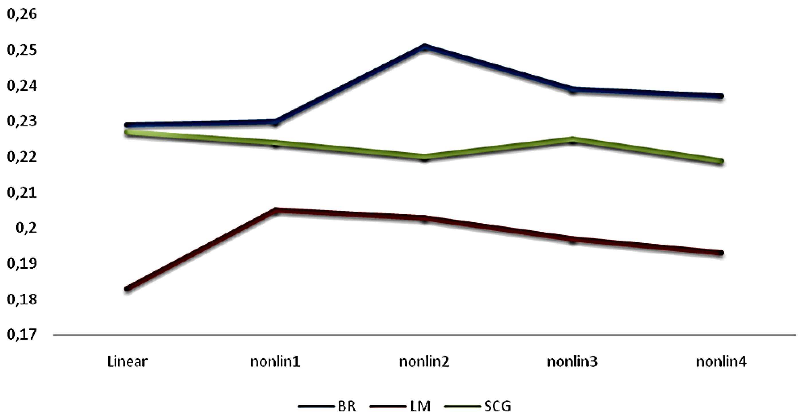
Training Algorithm	Linear	Nonlinear (One-Neuron)	Nonlinear (Two-Neuron)	Nonlinear (Three-Neuron)	Nonlinear (Four-Neuron)
BR	0.229	0.23	0.251	0.239	0.237
LM	0.183	0.205	0.203	0.197	0.193

and Figure 2, the correlation coefficients are summarized in order to see the predictive ability more clearly.

Table 4 shows that BR has the best predictive ability for both linear and nonlinear architectures. In this empirical study, a higher SSE and a lower correlation coefficient have been obtained by the LM. Figure 2 shows that the optimal model can be defined with two-neuron architecture in BRANN. Due to its predictive ability, using two-neuron architecture with BRANN was shown to be more reliable and robust. So, for clarity of the findings, the importance of the predictors was tested just with BRANN, not with LM.

Determining the importance of independent variables with the BR training algorithm is shown in

Table 5. The relative importance of predictors with different architectures of BRANN.

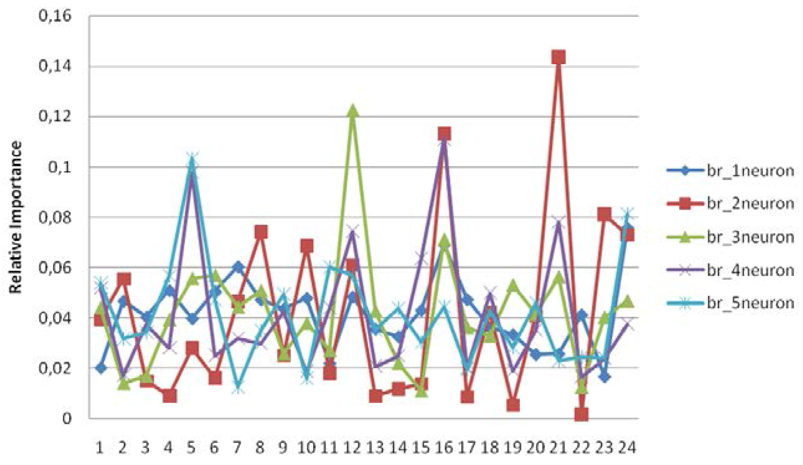
Predictors	Br_1neur.	Pred.	Br_2neur.	Pred.	Br_3neur.	Pred.	Br_4 neur.	Pred.	Br_5neur.
24	0.075826	21	0.14369	12	0.12251	16	0.1111	5	0.10333
16	0.069195	16	0.11314	16	0.07112	5	0.09779	24	0.08138
7	0.060357	23	0.08125	6	0.05684	21	0.07807	11	0.06017
4	0.050891	8	0.07418	21	0.05631	12	0.07447	12	0.05692
6	0.050532	24	0.07294	5	0.0556	15	0.06365	4	0.05661
12	0.048386	10	0.06862	19	0.05302	1	0.05183	1	0.05389
10	0.047885	12	0.06106	8	0.05076	18	0.04997	9	0.04936
17	0.047311	2	0.05554	24	0.04671	11	0.04395	6	0.04713
8	0.047199	7	0.04651	7	0.04425	9	0.04257	20	0.04578
2	0.046716	18	0.04221	1	0.04406	3	0.03772	16	0.04452
9	0.043606	20	0.04074	13	0.04253	24	0.0376	14	0.04377
15	0.043048	1	0.03932	20	0.04133	20	0.03522	18	0.04253
22	0.041268	5	0.02792	23	0.04024	7	0.03193	13	0.03518
3	0.040365	9	0.02497	4	0.03922	8	0.02974	8	0.03504
5	0.039735	11	0.01811	10	0.03784	4	0.02808	3	0.03427
18	0.036124	6	0.01616	17	0.03607	6	0.02513	2	0.03183
13	0.035587	3	0.0148	18	0.03285	14	0.02483	15	0.03038
19	0.033427	15	0.01372	11	0.02699	23	0.02402	19	0.02815
14	0.032593	14	0.01176	9	0.0256	13	0.02075	22	0.02449
21	0.025644	4	0.00903	14	0.02197	17	0.02022	23	0.02403
20	0.025484	13	0.00885	3	0.01687	19	0.019	21	0.02313
11	0.021935	17	0.00847	2	0.01394	10	0.01868	17	0.01958
1	0.020202	19	0.00538	22	0.01239	2	0.01712	10	0.01605
23	0.016684	22	0.00162	15	0.01097	22	0.01656	7	0.01249

where the effects of predictors are revealed according to priorities. The model was tested with one-, two-, three-, four-, and five-neuron architectures. The connection weight matrix of the neural network can be used to assess the relative importance of the various input neurons on the output [28,29]. The relative importance of the predictors (input factors) was calculated as below.

$$Ij=\frac{{{\displaystyle \sum }}_{i=1}^h\left((|W_{ji}|/{{\displaystyle \sum }}_{k=1}^n|W_{ki}|).|W{O}_i|\right)}{{{\displaystyle \sum }}_{k=1}^n\{{{\displaystyle \sum }}_{i=1}^h(|W_{ki}|/{{\displaystyle \sum }}_{k=1}^n|W_{ki}|).|W{O}_i|\}}$$

(13)

where Ij is the relative importance of the input factors j for the output, n is the number of input factors, h is the number of hidden neurons, W is the synaptic weight matrix between the input and the hidden layer, and WO is the synaptic weight matrix between the hidden and output layers [28,30].

Table 5 and Figure 3 show the relative importance of 24 input neurons upon the target for BR models. According to the findings, there is no serious difference among architectures in terms of predictive ability. The performance of the two-neuron architecture is slightly better, however, this difference is not significant. A model that has a complex structure cannot be explained with a single neuron in terms of revealing the relationships between predictors and target. Since complex models are penalized in accordance with the Bayesian approach, this approach is able to explore complex architecture [3]. All in all, the model with two-neurons is the best architecture because of the highest importance level of predictors. According to two-neuron architecture, the most important predictor is “Taking notes during lesson regularly”, with a relative index of 14.36%. The other important predictors are “Section being read from newspaper”, “Expected lesson’s details just from teacher”, “Completed preschool education”, and “Research Anxiety Score”, as can be seen in Table 5. In the architecture with three-, four-, and five-neurons, the relative indexes are lower than the two-neuron architecture. Therefore, the best model should be defined with two-neurons by using BRANN in this study.

4. Conclusions

The objective of this work is to demonstrate the predictive abilities of BR and LM neural network training algorithms. The ability to predict reflective thinking in the data was employed with two different backpropagation-based algorithms (BR and LM). The model was tested as both linear and nonlinear for BR and LM, separately. It was observed that the relationship between input and output neurons was nonlinear. To put the best nonlinear architecture forward, the model was tested with one-neuron architecture, two-, three-, four-, and five-neuron architectures. The best model was obtained according to the highest correlation coefficient between predicted and real data sets. The best model was scrutinized by BRANN not only by examining the highest correlation but also examining the least effective number of parameters. The other indicators of the best architecture were the SSE and SSW for BRANN.

Between the BRANN and LM training methods, the BRANN obtained the highest correlation coefficient and the lowest SSE in terms of predictive ability. The LM training algorithm showed lower performance in terms of predictive ability. Similarly, Okut et al. (2011) [3] proved that the BR training algorithm was the most effective method in terms of predictive ability.

Okut et al. (2013) [24] investigated the predictive performance of BR and scale conjugate gradient training algorithms. In their study, they found that the BRANN gave slightly better performance, but not significantly so. In many studies [8,31,32,33], the BR training algorithm has given either moderate or the best performance in terms of comparison with other training algorithms. BRANNs have some important advantages, such as choice and robustness of model, choice of validation set, size of validation effort, and optimization of network architecture [13]. Bayesian methods can solve the overfitting problem effectively and complex models are penalized in the Bayesian approach. In contrast to conventional network training, where an optimal set of weights is chosen by minimizing an error function, the Bayesian approach involves a probability distribution of network weights [21,34].

If data type (scale, nominal, ordinal) and distribution type of any data set is similar to the current data set then it is expected to have close results. For social data, it is possible to generalize the BRANN performance. Because Cross-Validation sampling enhances the findings and the sample was run many times to generalize the findings, it is concluded that among learning algorithms mentioned in this study, the BR training algorithm has shown better performance in terms of accuracy. This, combined with its advantage of having the potential ability to capture nonlinear relationships, means it can be used in quantitative studies to provide a robust model.

References

- Alaniz, A.Y.; Sanchez, E.N.; Loukianov, A.G. Discrete-time adaptive back stepping nonlinear control via high-order neural networks. IEEE Trans. Neural Netw. 2007, 18, 1185–1195. [Google Scholar] [CrossRef] [PubMed]
- Khomfoi, S.; Tolbert, L.M. Fault diagnostic system for a multilevel inverter using a neural network. IEEE Trans Power Electron. 2007, 22, 1062–1069. [Google Scholar] [CrossRef]
- Okut, H.; Gianola, D.; Rosa, G.J.M.; Weigel, K.A. Prediction of body mass index in mice using dense molecular markers and a regularized neural network. Genet. Res. Camb. 2011, 93, 189–201. [Google Scholar] [CrossRef] [PubMed]
- Vigdor, B.; Lerner, B. Accurate and fast off and online fuzzy ARTMAP-based image classification with application to genetic abnormality diagnosis. IEEE Trans. Neural Netw. 2006, 17, 1288–1300. [Google Scholar] [CrossRef] [PubMed]
- Gianola, D.; Okut, H.; Weigel, K.A.; Rosa, G.J.M. Predicting complex quantitative traits with Bayesian neural networks: A case study with Jersey cows and wheat. BMC Genet. 2011, 12, 1–37. [Google Scholar] [CrossRef] [PubMed]
- Moller, F.M. A scaled conjugate gradient algorithm for fast supervised learning. Neural Netw. 1993, 6, 525–533. [Google Scholar] [CrossRef]
- Hagan, M.T.; Menhaj, M.B. Training feedforward networks with the Marquardt algorithm. IEEE Trans. Neural Netw. 1994, 5, 989–993. [Google Scholar] [CrossRef] [PubMed]
- Saini, L.M. Peak load forecasting using Bayesian regularization, Resilient and adaptive backpropagation learning based artificial neural networks. Electr. Power Syst. Res. 2008, 78, 1302–1310. [Google Scholar] [CrossRef]
- Beal, M.; Hagan, M.T.; Demuth, H.B. Neural Network Toolbox™ 6 User’s Guide; The Math Works Inc.: Natick, MA, USA, 2010; pp. 146–175. [Google Scholar]
- Mackay, D.J.C. Bayesian interpolation. Neural Comput. 1992, 4, 415–447. [Google Scholar] [CrossRef]
- Demuth, H.; Beale, M. Neural Network Toolbox User’s Guide Version 4; The Math Works Inc.: Natick, MA, USA, 2000; pp. 5–22. [Google Scholar]
- Bishop, C.M.; Tipping, M.E. A hierarchical latent variable model for data visualization. IEEE Trans. Pattern Anal. Mach. Intell. 1998, 20, 281–293. [Google Scholar] [CrossRef]
- Burden, F.; Winkler, D. Bayesian regularization of neural networks. Methods Mol. Biol. 2008, 458, 25–44. [Google Scholar] [PubMed]
- Marwalla, T. Bayesian training of neural networks using genetic programming. Pattern Recognit. Lett. 2007, 28, 1452–1458. [Google Scholar] [CrossRef]
- Titterington, D.M. Bayesian methods for neural networks and related models. Stat. Sci. 2004, 19, 128–139. [Google Scholar] [CrossRef]
- Felipe, V.P.S.; Okut, H.; Gianola, D.; Silva, M.A.; Rosa, G.J.M. Effect of genotype imputation on genome-enabled prediction of complex traits: an empirical study with mice data. BMC Genet. 2014, 15, 1–10. [Google Scholar] [CrossRef] [PubMed]
- Alados, I.; Mellado, J.A.; Ramos, F.; Alados-Arboledas, L. Estimating UV erythemal irradiance by means of neural networks. Photochem. Photobiol. 2004, 80, 351–358. [Google Scholar] [CrossRef] [PubMed]
- Mackay, J.C.D. Information Theory, Inference and Learning Algorithms; University Press: Cambridge, UK, 2008. [Google Scholar]
- Sorich, M.J.; Miners, J.O.; Ross, A.M.; Winker, D.A.; Burden, F.R.; Smith, P.A. Comparison of linear and nonlinear classification algorithms for the prediction of drug and chemical metabolism by human UDP-Glucuronosyl transferesa isoforms. J. Chem. Inf. Comput. Sci. 2003, 43, 2019–2024. [Google Scholar] [CrossRef] [PubMed]
- Xu, M.; Zengi, G.; Xu, X.; Huang, G.; Jiang, R.; Sun, W. Application of Bayesian regularized BP neural network model for trend analysis. Acidity and chemical composition of precipitation in North. Water Air Soil Pollut. 2006, 172, 167–184. [Google Scholar] [CrossRef]
- Mackay, J.C.D. Comparison of approximate methods for handling hyperparameters. Neural Comput. 1996, 8, 1–35. [Google Scholar] [CrossRef]
- Kelemen, A.; Liang, Y. Statistical advances and challenges for analyzing correlated high dimensional SNP data in genomic study for complex. Dis. Stat. Surv. 2008, 2, 43–60. [Google Scholar]
- Gianola, D.; Manfredi, E.; Simianer, H. On measures of association among genetic variables. Anim. Genet. 2012, 43, 19–35. [Google Scholar] [CrossRef] [PubMed]
- Okut, H.; Wu, X.L.; Rosa, G.J.M.; Bauck, S.; Woodward, B.W.; Schnabel, R.D.; Taylor, J.F.; Gianola, D. Predicting expected progeny difference for marbling score in Angus cattle using artificial neural networks and Bayesian regression models. Genet. Sel. Evolut. 2013, 45, 1–8. [Google Scholar] [CrossRef] [PubMed]
- Foresee, F.D.; Hagan, M.T. Gauss-Newton approximation to Bayesian learning. In Proceedings of the IEEE International Conference on Neural Networks, Houston, TX, USA, 9–12 June 1997; pp. 1930–1935.
- Shaneh, A.; Butler, G. Bayesian Learning for Feed-Forward Neural Network with Application to Proteomic Data: The Glycosylation Sites Detection of The Epidermal Growth Factor-Like Proteins Associated with Cancer as A Case Study. In Advances in Artificial Intelligence; Canadian AI LNAI 4013; Lamontagne, L., Marchand, M., Eds.; Springer-Verleg: Berlin/Heiddelberg, Germany, 2006. [Google Scholar]
- Souza, D.C. Neural Network Learning by the Levenberg–Marquardt Algorithm with Bayesian Regularization. Available online: http://crsouza.blogspot.com/feeds/posts/default/webcite (accessed on 29 July 2015).
- Bui, D.T.; Pradhan, B.; Lofman, O.; Revhaug, I.; Dick, O.B. Landslide susceptibility assessment in the HoaBinh province of Vieatnam: A comparison of the Levenberg–Marqardt and Bayesian regularized neural networks. Geomorphology 2012, 171, 12–29. [Google Scholar]
- Lee, S.; Ryu, J.H.; Won, J.S.; Park, H.J. Determination and application of the weights for landslide susceptibility mapping using an artificial neural network. Eng. Geol. 2004, 71, 289–302. [Google Scholar] [CrossRef]
- Pareek, V.K.; Brungs, M.P.; Adesina, A.A.; Sharma, R. Artificial neural network modeling of a multiphase photo degradation system. J. Photochem. Photobiol. A Chem. 2002, 149, 139–146. [Google Scholar] [CrossRef]
- Bruneau, P.; McElroy, N.R. LogD7.4 modeling using Bayesian regularized neural networks assessment and correction of the errors of prediction. J. Chem. Inf. Model. 2006, 46, 1379–1387. [Google Scholar] [CrossRef] [PubMed]
- Lauret, P.; Fock, F.; Randrianarivony, R.N.; Manicom-Ramsamy, J.F. Bayesian Neural Network approach to short time load forecasting. Energy Convers. Manag. 2008, 5, 1156–1166. [Google Scholar] [CrossRef]
- Ticknor, J.L. A Bayesian regularized artificial neural network for stock market forecasting. Expert Syst. Appl. 2013, 14, 5501–5506. [Google Scholar] [CrossRef]
- Wayg, Y.H.; Li, Y.; Yang, S.L.; Yang, L. An in silico approach for screening flavonoids as P-glycoprotein inhibitors based on a Bayesian regularized neural network. J. Comput. Aided Mol. Des. 2005, 19, 137–147. [Google Scholar]