
A Computational Fluid Dynamic Study of Developed Parallel Stations for Primary Fans


1
Departamento de Ingeniería en Minas, Facultad de Ingeniería, Universidad de Santiago, Santiago 9160000, Chile
2
Bharti School of Engineering, Laurentian University, Sudbury, ON P3E 2C9, Canada
*
Author to whom correspondence should be addressed.
Processes 2021, 9(9), 1607; https://doi.org/10.3390/pr9091607
Submission received: 30 June 2021
/
Revised: 30 August 2021
/
Accepted: 31 August 2021
/
Published: 8 September 2021
(This article belongs to the Special Issue Applied Computational Fluid Dynamics (CFD))
Abstract
:A Computational fluid dynamic (CFD) model was developed considering three geometries for primary parallel fan stations that have already been developed, implemented, and are currently in operation within Chilean mines. To standardize the comparison, the same primary fan was used in all the simulations with a unique set of settings (speed, blade angle, and density). The CFD representation was used to determine the operating point per configuration and compare the performances in terms of airflow and pressure delivered. This approach allowed ranking primary fan station geometry based on resistance curve and energy consumption of the fan. This paper presents the results obtained through the CFD simulations and the corresponding primary fans operating points of each configuration: symmetrical branches (SB), overlap branches (OB), and run around (RA) bypass. The RA configuration was identified as the best-performing station geometry on the lowest frictional and shock pressure losses, highest airflow delivery, and lowest energy cost. The results are discussed, considering pressure, velocity, and vector contours to understand the fluid dynamics phenomena occurring inside the station. The capital cost involved in the development of each primary parallel station was considered in the analysis in addition to the energy cost to determine the economic configuration over time.
1. Introduction
Operators of underground mines are looking for options to increase production rates and improve the competitiveness of the business by offsetting increased costs from the depletion of surface deposits and the greater depth of new deposits. This can lead to the use of a larger or bigger diesel equipment fleet working underground or a combination of both. The airflow volume requirements of the work faces increase as a proportion of the additional diesel horsepower, resulting in an increased airflow requirement for the complete mine, for the primary fresh air and return air systems.
Using the mine plan, the associated diesel fleet, and regulations for underground environments as an input, the airflow volume requirements are estimated for the mine over time. Then based on the mine design and schedule, a ventilation plan is formulated that includes the main and auxiliary fans. The main intake and exhaust fans and controls such as ventilation doors, fire doors, and regulators are then sized and located in the mine layout over time to provide the mine plan airflow volumes needed for development and production activities.
Parallel fan stations are used when the amount of air needed inside the mine is of such a magnitude that one fan fails to meet this demand, or an additional fan is required to cover maintenance periods. Fans installed in galleries arranged in parallel allow the generation of a similar pressure in both fans while sharing the airflow volume. An advantage of using two identical fans in parallel is that if one of them fails, or is down for maintenance, then the remaining fan continues to supply a significant portion of the original flow, up to 70% [1,2].
In the past, modeling of parallel fan station performance has been performed using analytical and ventilation software tools. In recent years, computational fluid dynamics (CFD) have been used to model areas of interest within ventilation models, in particular, unsmooth geometries such as fan stations [3]. According to Versteeg and Malalasereka 1995 [4], CFD is the analysis of systems involving fluid flow, heat transfer, and associated phenomena such as chemical reactions by means of computer-based simulation.
The application of CFD has been proposed for the simulation and comparison of shock losses in underground mine ventilation systems [5]. CFD simulation has also been applied to ventilation shock losses in production drifts and parallel fan stations [6,7,8,9]. However, the results were neither definitive nor comparative since the conditions evaluated were for a single geometry in each study.
In the previously mentioned literature, the theoretical basis and conditions for the simulation of parallel fan stations with CFD were provided. Unfortunately, and due to the limitation of exploring a single geometry, more work is required to understand the fan performance variation depending on the station geometry design.
The study of the parallel fan ventilation stations developed in this paper considers three different geometries, all of them currently in use for underground mining in Chile. Due to the heterogeneity of their construction, it was necessary to establish the dynamic fluid characteristics of each design so as to discuss the advantages or disadvantages of each fan station configuration and then determine the most energy-efficient one.
This paper presents guidelines for the geometry characteristics that need to be considered for three particular parallel ventilation station designs containing two fans. The designs are compared according to fan operating points, energy consumption, and differences in the systematic resistance they present under standard conditions. Furthermore, the analysis is extended considering the capital expenditure required for developing these geometric designs and estimating the net present value generated over additional time to only considering the energy cost.
2. Methodology
The three two-fan parallel ventilation station geometries are modeled and simulated with Ansys-Fluent 16.0 computational fluid dynamic software to determine the fans’ operational points. The objective was to find which parallel fan station geometry would obtain the best fan operational point, i.e., deliver the highest flow rate and lowest static pressure, resulting from the lowest equivalent resistance curve of the parallel fan station configuration under the same fan conditions (speed, blade angle, and altitude or density).
In order to perform a dynamic fluid comparison of the stations’ designs, it is necessary to establish some similar characteristics in the models because each working fan station uses a different fan. This is why a standardized fan was used for all configurations. The fan selected was an axial fan, model Alphair 1480 AMF 6600, with the blade angle set to 20°, equipped with an impeller of 4 m diameter, an inlet bell on the suction, and a diffuser on the discharge side. The fan curve at the specified blade angle setting had a maximum airflow volume of 470 m3/s and 1890 Pa maximum static pressure [6]. As the resistance of the galleries depends on their geometric characteristics, a common cross-sectional airway area was used for all models, namely 7.2 m × 7.2 m. Figure 1a shows the fan’s characteristic curves for its range of blade angles, and Figure 1b shows the individualized flow curve (red) and power (blue) selected for the fan with a 20° blade setting angle. The units are different between both curves because the original manufacturer’s curve is in the Imperial System (a), while the chosen curve (b) for the simulation has been converted to the International Unit System for this study.
3. Computational Domain
The three parallel fan ventilation station configurations considered in this study were named as follows:
As previously mentioned, all fans station configurations have 7.2 m × 7.2 m (width and height) with a shoe horse shape of drift.
3.1. Symmetrical Branches
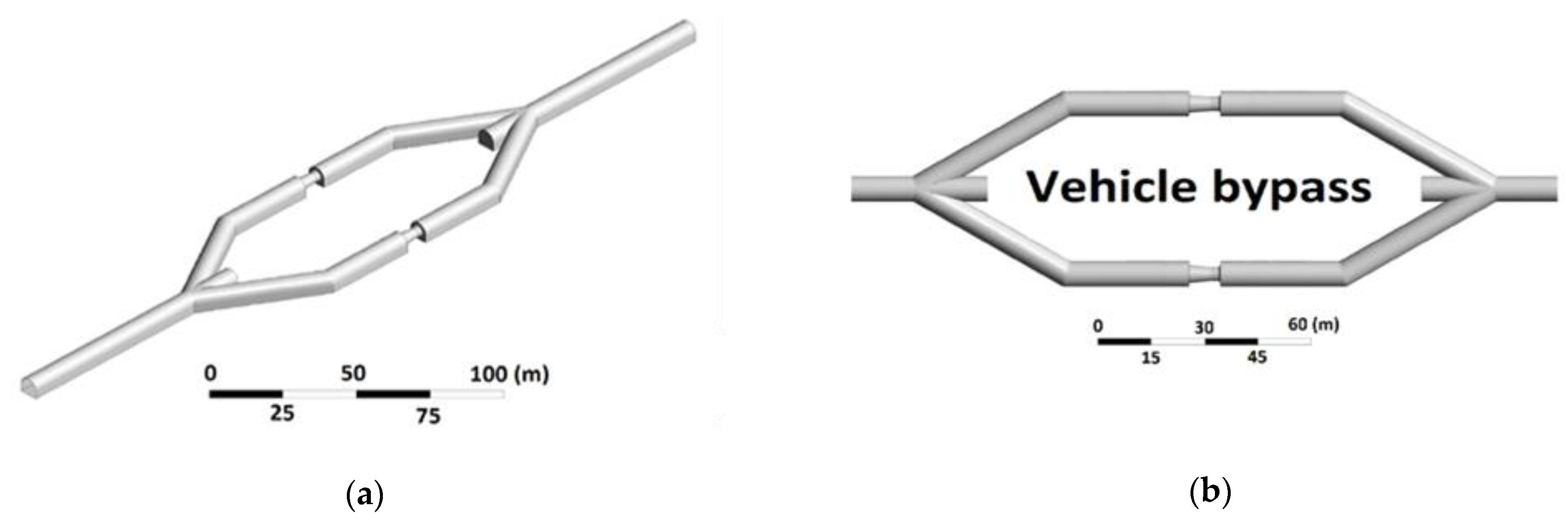
This model consists of six singularities: one opening at 60° ‘Y’, two 30° elbows in series in each branch, and one closing at 60° ‘Y’. In addition, the station has a central gallery to allow for personnel or vehicle movement (vehicle bypass), which is truncated for simplicity, reflecting the existence of ventilation airlocks that prevent significant airflow recirculation. The initial and final straight sections measure 70 m each. The four diagonal sections that are part of the opening and closing ‘Y’ measure 51.5 m each. The straight parallel sections of the tunnel where the fans are located measure 85.5 m each. This configuration presents a total construction length of 517 m and is based on the layout used at the El Teniente Mine. In this analysis, only the center lines were considered for the construction of the fan station geometrical model. The actual mine layout had different size galleries and fans. The physical characteristics of the model are illustrated in Figure 2.
3.2. Overlapped Branches
This configuration is very similar to the parallel branches, but it has the peculiarity that the opening ‘Y’ and the closing ‘Y’ branches are displaced by 6.5 m, and its angle is 90°. The two elbows in each branch are 45°. This geometry also presents the transit gallery through the middle of the ventilation station equipped with an airlock. The initial and final straight sections measure 70 m each. The four diagonal sections that are part of the opening and closing ‘Y’ measure 36 m each. The straight parallel sections of the tunnel where the fans are located measure 47.5 m each. This station has a construction length of 379 m, which makes it the shortest ventilation station arrangement studied. It presents more abrupt singularities and shorter distances for flow stabilization leading to and from the fan, as presented in Figure 3.
3.3. Run Around
This configuration consists of a main straight gallery with an opening gallery at 30°, two 30° elbows, and a closing intersection at 30°. The initial and final straight sections measure 70 m each. The two diagonal sections that are part of the opening and closing ‘Y’ measure 48 m each. The straight parallel sections of the tunnel where the fans are located measure 79 m and 164 m, respectively. The station comprises 479 m of gallery constructed between the main and the bypass branches. The gallery for vehicle and pedestrian traffic is an additional bypass with airlocks located in the bypass branch, as presented in Figure 4.
This configuration was designed and studied previously by [6] for the New Level Mine project for the El Teniente mine. It was proposed as a solution for the ventilation design to achieve the airflow volume increase during the development phase without having to develop a new complete return airway to the surface.
4. Boundary Conditions
Boundary conditions are a necessary component for the solution of the fluid-dynamic mathematical models as they define the value of the differential equation adopted at the edge of the domain. In this study, three main boundary conditions were used: Fan, Outlet Vent, and Wall. The Fan boundary condition is a plane that assigns the fan characteristic curve, point by point, to a surface (3D models) by means of defined points with average speed and static pressure. With this boundary condition, it is not necessary to simulate the fan blades nor to assign rotational speed because the performance curve automatically adapts the conditions according to resistance. Outlet Vent BC allows the modeling of an obstruction surface (or line for 2D) to which a flow resistance is assigned (like an orifice plate type) and regulated by the coefficient of loss K, which is proportional to the dynamic pressure. The loss of coefficients ‘K’ to define the resistance of the system is defined as a shock loss factor, which is shown in the following Equation (1):
where ∆P is the pressure differential, K is the shock loss factor, is the density and u is the velocity. This boundary condition is used in the input (inlet) and outlet (geometry), which allows for adjustment of the operating point of the fan by changing the coefficients of loss K.
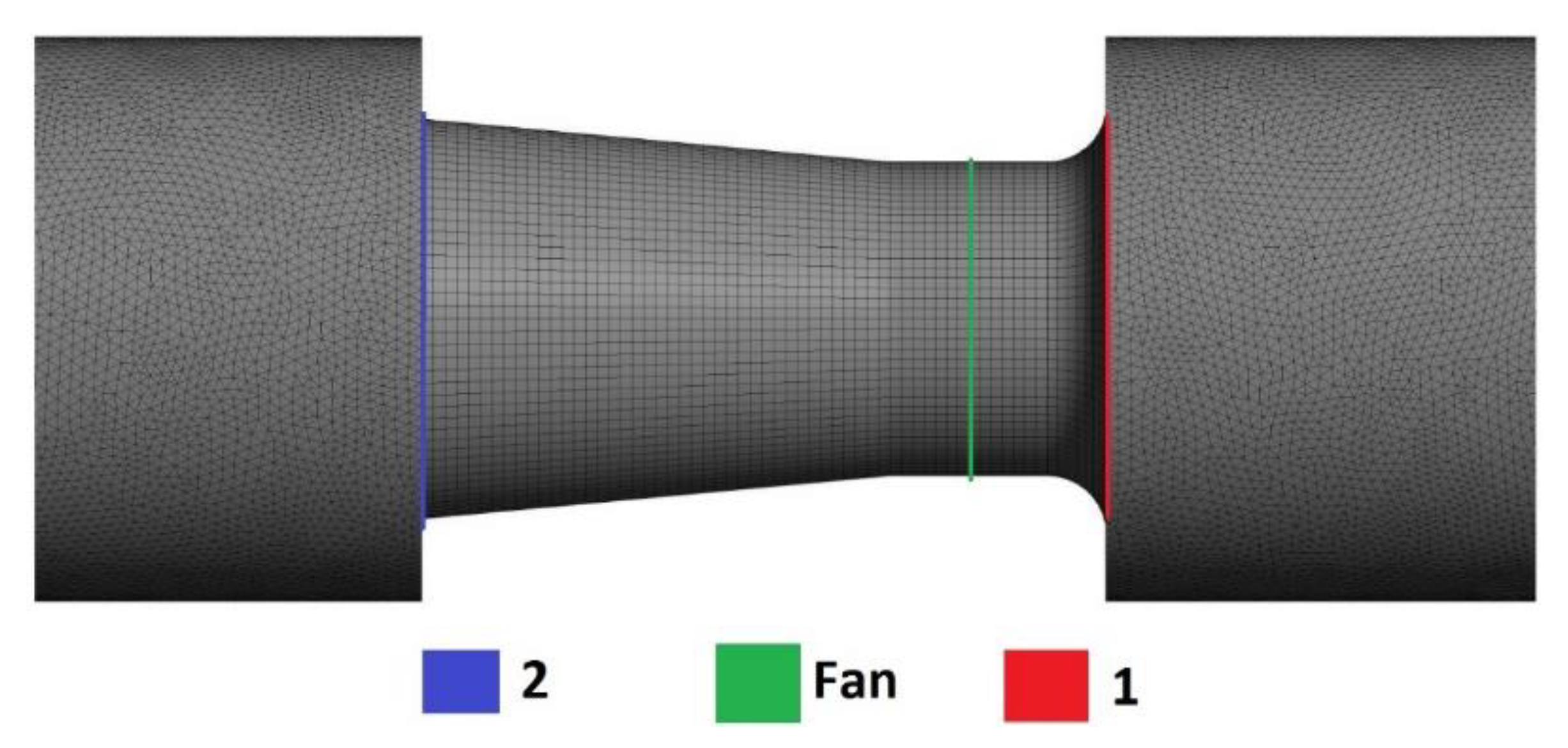
The Wall BC is adopted for each solid wall present in the geometry. In viscous flows, the tangential velocity of the fluid is equal to that of the wall, while the velocity in its normal component is zero. The wall condition is used to assign a roughness to the walls of the ventilation stations, which for this study is the same for all drifts. Figure 5 shows the location of boundary conditions in the proposed geometry.
5. Set up and Initial Conditions
The solver was based on isothermal, incompressible, and unsteady conditions, with a time step of 5 × 10⁻² s [10]. The number of steps was 520, and the resulting 26 s of flow time. The initial conditions are the physical characteristics of the stations in the simulation. In this case, the resistance of the system is varied, whereas the aforementioned variables are defined by default as ideal conditions at 15 °C and an atmospheric pressure of 101,325 Pa. Table 1 presents the loss coefficients for fan ventilation stations to set the operating points. Residuals were set to 10−5.
‘K’ values presented in Table 1 are used to replicate upstream and downstream resistance simulating different operating points. For practical case analysis, the mid-point of the fan operational curve has been selected as the initial operating condition. This point was chosen because it is far from the stagnation zone and is also located in an area with an approximate efficiency of 70% [2,6].
The turbulence model selected was k-ԑ Realizable according to previous work developed [10]. Computation was solved with SIMPLEC scheme for the pressure-velocity coupling, second-order upstream discretization for pressure, Third-Order MUSCL for momentum and turbulent dissipation rate, and QUICK for turbulent kinetic energy.
5.1. Obtaining the Operational Point
In order to describe the operation points of the fan stations, the static pressure [6] was used, and Figure 6 is obtained according to the following Equation (2):
where Pfan static is the static pressure of the fan, Ptotal inlet(1) is the total pressure at the inlet, and Pstatic outlet(2) is the static pressure at the outlet.
The flow rate was established directly at the fan outlet via a control surface (Figure 6, blue line). In addition, each fan was identified according to the position and direction of flow. In the plan view of the fans, the flow direction runs from left to right. Figure 7 shows the flow direction and fan arbitrary naming convention. The top one is ‘fan a’ and the bottom one ‘fan b’. Resistance is obtained by varying the Outlet Vent boundary condition, modifying the loss coefficient in the inlet (Kinlet) and outlet (Koutlet) (see Figure 5).
5.2. Mesh
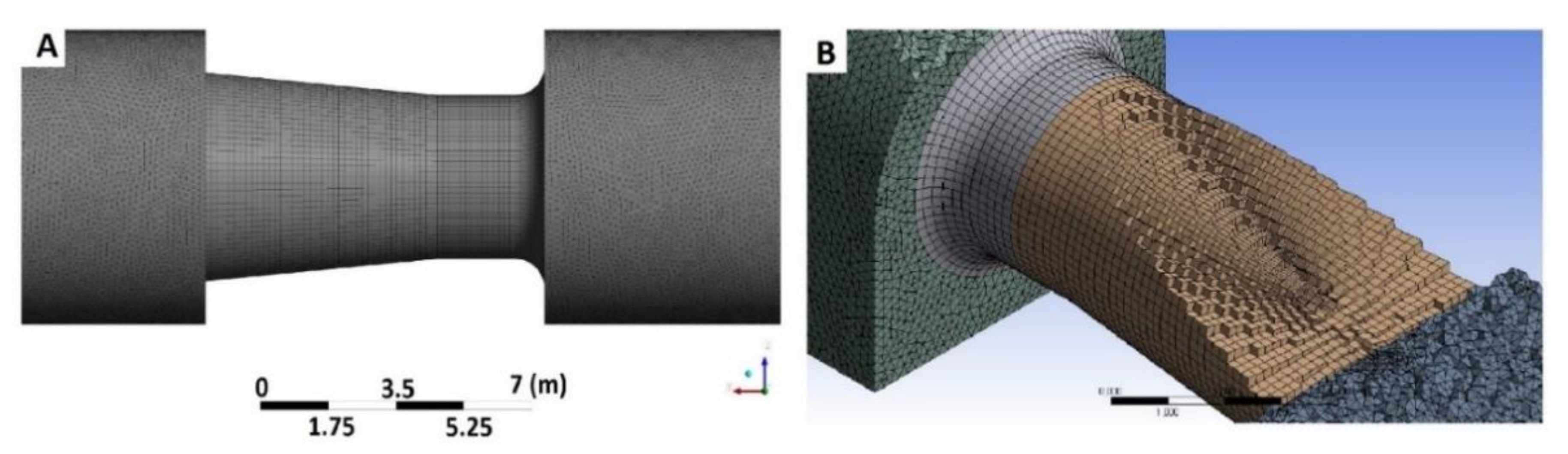
Based on the previous works developed [6,10] with similar geometries, the mesh test size and its analysis developed are applicable to this work. The cell size for the fan zones and in its vicinity corresponds to a 10 cm cell size. In the drifts, it was defined as a constant 50 cm for the stations, obtaining an approximate total of six million cells as presented in Figure 8.
6. Results
6.1. Operational Points
Table 2 shows the operational points for the symmetrical branches (SB), overlapped branches (OB), and run around (RA) configurations at different resistance points of the ventilation system with their respective operation graph in Figure 9.
To compare the different configurations, common resistance states (Kinlet-Koutlet: 7.5–15, 0–6.5, and 0–0) are defined in Figure 9, where Figure 9a represents the total flow and pressure of the stations while Figure 9b represents the fans individually.
To center the comparison, the average resistance of the curve with edge condition Kinlet = 0 and Koutlet = 6.5 is used [2,6]. The results are shown in Figure 10, where the operating point of the fans within the stations is compared. It can be observed that the operating point of the run around (RA) configuration is the geometry with higher flow and lower pressure, followed by the overlapped branches configuration.
Figure 11 allows observing the resistance curves for the three configurations under the boundary condition of medium resistance, with a clear differentiation in its curve of total resistance for each station. Figure 11a shows the complete curve of the fan, and Figure 11b shows an approach to the operating points of each fan configuration.
The operational point of a fan is the intersection of the resistance curve and the fan curve. The resistance that the fan station experiences, also referred to as Atkinson’s resistance, can be determined by using the ‘’Square law of mine ventilation’’ [1,2], which states that pressure differential is equal to the resistance times the square of the airflow. With the obtained CFD operational point (pressure and airflow), the resistance value is determined and then used to plot the resistance curve.
6.2. Computational Fluid Dynamics Analysis
Figure 12 and Figure 13 show the velocity vectors, given in the plan view, for each fan station and for the separations and junctions of the flow, respectively, according to each configuration. The block on the left side of each plot represents the fan motor. Figure 14 shows a full plan view of the velocities through each station configuration. Similarly, a static pressure plan profile is shown in Figure 15 for each complete configuration. Although Figure 15 shows a relatively homogeneous pressure distribution, the other Figure 12, Figure 13 and Figure 14 show that the flow entering some of the fans is unbalanced. This is due to upstream singularities such as gaps, geometric misalignments, elbows, and their interactions, which affect the operational point of each fan.
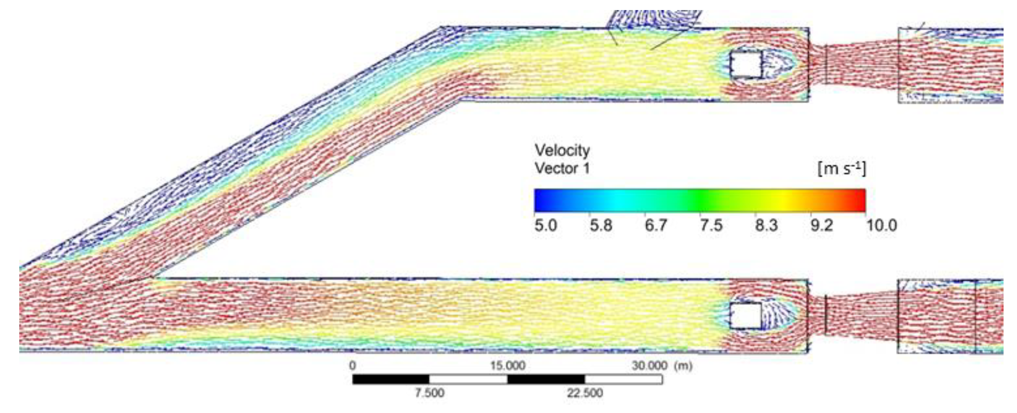
For the run around configuration, the fan with the best operational point and higher flow rate is ‘fan b’. This is because this fan has one distant separation of 70 m upstream, which allows the flow to fully develop before entering the fan. A close inspection of the run around ‘fan a’ velocity vector in Figure 12 (RA a) shows that it has double equally sized vortices downstream from the motor assembly, indicating a relatively homogenous flow entering from both sides of the fan inlet. The remaining fans in Figure 12, including ‘fan b’ of the run around arrangement, show varying levels of inhomogeneity in the flows entering the fans. The flow-through ‘fan a’ of the run around configuration has to travel a longer distance and go through two counter elbows, but it appears to help to order the airflow stream before entering the fan, although it slightly affects its operating point such as shown in Figure 10. To better demonstrate this phenomenon, in Figure 16, the colored velocity vectors are shown according to a bounded velocity scale to present differences in the drift flow velocity prior to entering the fans. Apparently, the two singularities (elbow and counter elbow) prior to the ‘fan a’ entry allow the airflow to align properly, whereas in ‘fan b’, the flow does not reach the same level of alignment. It is important to notice that it is a three-dimensional simulation, and the vortices involved have an important vertical component.
On the other hand, symmetrical branches are the traditional “Y” configuration used in fan stations in mines. It offers a more homogeneous operating point between its two fans but offers the highest resistance (Figure 10) for the cases analyzed. This is due to the larger opening angle between branches and the extensive length between the separation and junction nodes. It should be noted that a shorter length requires a greater opening angle, which would generate a greater shock loss. This is that of the overlapping branches (OB), whose configuration obeys a design based on operational experience to couple the start of the fans, which allows less interfered with each other. For this OB configuration, it is shown that, due to the higher angle of the singularities (elbows at 45°), in the suction branches, a large part of the flow is preferentially distributed towards the internal walls of the gallery and then homogenizes near the motor (Figure 14).
Overall, the resistance of the symmetrical branches’ arrangement is slightly higher than that of the overlapped branches circuit, although the latter has more acute angle bends and displaced joints and separations, which generate a more turbulent flow, as can be seen in Figure 12, Figure 13 and Figure 14. The reason for this is the 138 m less length of the overlapped branch configuration from the split point until the union point of the branches. As a result, the reduction in linear losses would more than compensate for the higher turbulent losses of the configuration of this station. As previously mentioned, these are mine site operating configuration geometries, and as such, the intent of this study was not to compare equal fan stations lengths but to determine which geometry delivered the best performance.
6.3. Energy Consumption Analysis
Due to more representative operation points of fan curves is the mid-resistance (Kentry = 0, Koutlet = 6.5), it shall be analyzed particularly. There are differences in the total resistance curves of the system between the different configurations, even though they were subjected to the same boundary and initial conditions, indicating that the configuration of the station influences the fan performance just like a singularity as expected. The resistance curves obtained for each of the stations, as given in Table 3, show that the run around configuration has the lowest resistance at 0.00201 kg s2/m8, and the symmetrical branch had the highest resistance at 0.00236 kg s2/m8, an increase of 3.48 × 10⁻⁴ kg s2/m8 or 17%. The overlap branch arrangement fell midway between these two arrangements.
Figure 9 shows that the working range of the fan is dominated by a decreasing power with the flow rate. Table 4 shows the variation in total consumed power per two-fan station at different points of the fan curve across the different configurations. This table shows that RA consumes more energy than the other arrangement at low flow rates but becomes the lowest energy user at high flow rates. If the annual consumption of these differences is quantified (Table 5) in terms of energy consumption, it can be seen that the run around station obtains a lower consumption with a slight decrease in its operating point, which translates into a saving of at least 268 MWh annually compared to the other two geometries.
6.4. Energy and Development Cost Analysis
In the previous point, the analysis was developed only considering the energy cost of operating the fans and the most representative fan curve operation point, which is the mid-resistance (Xentry = 0, Xoutlet = 6.5). Nevertheless, the driving layout of the three geometries has different lengths, which motivated the need for a second analysis considering the capital cost of the development.
As presented in Table 2, for the mid-resistance (Xentry = 0, Xoutlet = 6.5), the yearly power requirement for SB, OB, and RA is 949 kW, 916 kW, and 883 kW, respectively. It was also indicated previously that the length of development from opening wye to closing wye for SB, OB, and RA is 517 m, 379 m, and 479 m, respectively.
From the numbers provided, it can be observed that the geometry SB is the one with the longest development length and energy consumption, making it the less desirable approach in terms of cost. However, a trade-off appears between the other two remaining geometries: OB and RA. OB has a higher yearly power consumption to operate than RA, but the development requires less meters and, as such, a smaller capital cost for construction. The question that remains to be answered is: what is the limit for the payback to be more interesting in one kind of scenario than the other?
The considered development cost for the proposed cross-section of 7.2 m by 7.2 m was 6500 USD per meter, and the energy cost was 150 USD/MWh. The interest rate considered was 8%. Considering both costs, energy, and development, the SB geometry was always the costlier one to implement. Between the OB and RA geometries, the latter was more expensive for a 20-year period payback consideration. However, this result is very sensitive to the balance between the energy cost and the development cost considered. The OB geometry would remain the less overall cost for the analysis, even if it were the geometry with the higher energy cost.
In terms of relative cost, the difference between the two overall costs was 15%, 6%, 4%, and 2% for the first, fifth, tenth, and twentieth year, respectively, as presented in Table 6.
When looking at the life of a mine (LOM) plan and when considering the main ventilation infrastructure to support that plan, the adequate range for payback can vary significantly. The main issue will remain the tendency to minimize the capital investment during the first years of development before the ore profit becomes available.
A common topic of interest in this kind of trade-off exercise is usually to know within which ranges of energy prices and development costs the OB geometry could become more convenient than the RA geometry using the NPV as a measure of goodness. Table 7 presents the sensitivity analysis of energy price and development cost, at which the RA geometry becomes a better investment for the mine site over the OB geometry. Table 7 indicates the number of years at which the OB geometry becomes a larger cost in terms of NPV.
As can be observed in Table 7, with the current length of the RA geometry, it requires between 19 to 39 years and an energy price of 200 to 250 USD/MWh to adopt it over the OB geometry. Then as the development cost is reduced, the trade-off becomes more favorable. The analysis performed considers a fixed cost of both energy and development over the time period considered. In Table 7, the boxes with no number of years represent all the cases in which the payback was over the 50 years.
Based on the results obtained for these three studied geometries, new questions develop, such as: What is the adequate balance between the development length and the energy consumption that a parallel ventilation station will have? The authors expect that further work in this research avenue will hopefully lead to a design optimization methodology for parallel fan stations, which now will consider the overall cost and not only the development cost as it might have been the case in the past.
7. Conclusions
This study presents an attempt to simulate and compare the performance of two-fan parallel stations, considering three different configurations or geometries. This allows one to determine the resistance and power consumption of each configuration and to estimate their energy performance when delivering a certain airflow volume and pressure drop. It was determined that the run around configuration has the best performance at higher airflow volumes. The results presented in this study suggest that the initial theoretical recommendation of constructing two-fan parallel stations as symmetrically as possible should be reviewed on a case-by-case basis. The work developed in this study also suggests that the run around is ranked as the best-performing geometry, mainly due to the reduced shock losses and relatively short ventilation drift length of this configuration when compared to the other two. The economic analysis indicates that the overlap branches, despite been the worst performer in terms of energy consumption, turned out to be the best performer when considering certain energy prices and development costs. Moreover, and depending on the energy and development cost considered, over time, the run around could potentially become the best alternative for the overall cost and not only the energy consumption.
In our future work, a series of studies will be required to compare the three geometries at the equivalent length of development and to quantify if the impact in shock losses could be overcome by the savings of reduced developments. Before defining a model of fan station, it is strongly recommended to set a CFD analysis of different options that consider geometrical, aerodynamic, and economic aspects over time.
Author Contributions
Conceptualization, J.P.H. and E.A.; Formal analysis, J.P.H., J.P.V. and E.A.; Investigation, G.R.; Project administration, J.P.V.; Software, G.R.; Writing—original draft, G.R.; Writing—review and editing, J.P.H. and E.A. All authors have read and agreed to the published version of the manuscript.
Funding
This research was funded by the Dirección de Investigaciones Científicas y Tecnológicas, Universidad de Santiago de Chile, Research Project number 051515HC executed at Universidad de Santiago de Chile. The APC was funded by the Departamento de Ingeniería en Minas de la Universidad de Santiago de Chile.
Conflicts of Interest
The authors declare no conflict of interest.
References
- Hartman, H.L.; Mutmansky, J.M.; Ramani, R.V.; Wang, Y.J. Mine Ventilation and Air Conditioning; John Wiley & Sons, Inc.: Toronto, ON, Canada, 1997. [Google Scholar]
- McPherson, M.J. Subsurface Ventilation and Environmental Engineering; Springer Science & Business Media: Berlin, Germany, 2012. [Google Scholar]
- Acuña, E.I.; Hurtado, J.P.; Wallace, K. A Summary of Computational Fluid Dynamic Application to the New Level Mine Project of El Teniente. In Proceedings of the 10th International Mine Ventilation Congress, Johannesburg, South Africa, 2–8 August 2014; pp. 91–97. [Google Scholar]
- Versteeg, H.; Malalasereka, W. An Introduction to Computational Fluid Dynamics: The Finite Volume Method, 1st ed.; Longman Scientific & Technical: Essex, UK, 1995. [Google Scholar]
- Diego, I.; Torno, S.; Toraño, J.; Menéndez, M.; Gent, M. A practical use of CFD for ventilation of underground works. Tunn. Undergr. Space Technol. 2011, 26, 189–200. [Google Scholar] [CrossRef]
- Hurtado, J.P.; Acuña, E.I. CFD analysis of 58 adit main fans parallel installation for the 2015–2019 underground developments of the New Level Mine project. Appl. Therm. Eng. 2015, 90, 1109–1118. [Google Scholar] [CrossRef]
- Hurtado, J.P.; Díaz, N.; Acuña, E.I.; Fernández, J. Shock losses characterization of ventilation circuits for block caving production levels. Tunn. Undergr. Space Technol. 2014, 41, 88–94. [Google Scholar] [CrossRef]
- Pan, J. Study on the local ventilation resistance of multistage fan stations. Met. Min. 2001, 9, 49–51. [Google Scholar]
- Gou, Y.; Shi, X.; Zhou, J.; Qiu, X.; Chen, X. Characterization and effects of the shock losses in a parallel fan station in the underground mine. Energies 2017, 10, 785. [Google Scholar] [CrossRef] [Green Version]
- Llanca-Pacheco, J.L. Determinación de la Interferencia en la Incorporación de un Ventilador en Paralelo, Proyecto Nuevo Nivel Mina; Tesis para Optar al Titulo de Ingeniero de Ejecución en Minas; Universidad de Santiago de Chile, Facultad de Ingeniería, Departamento de Ingeniería en Minas: Santiago, Chile, 2013. [Google Scholar]
Figure 1.
(a) Fan characteristic curves; (b) CFD calibrated and simulated fan curve and hydraulic power curve for a 20° blade angle.
Figure 1.
(a) Fan characteristic curves; (b) CFD calibrated and simulated fan curve and hydraulic power curve for a 20° blade angle.
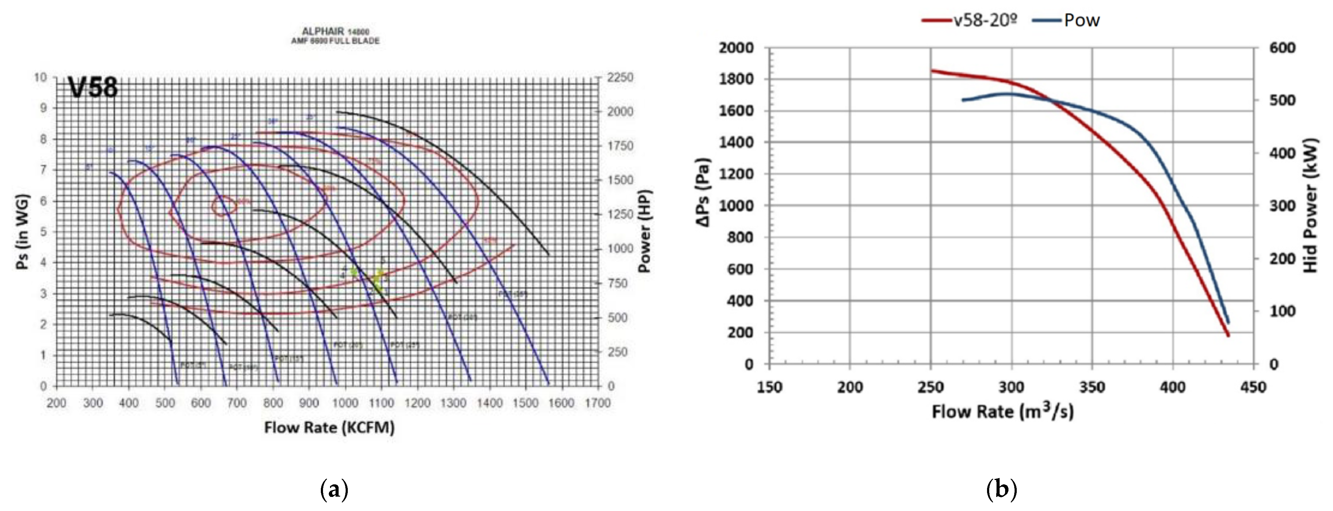
Figure 2.
Symmetrical branches parallel fan station 3D model; (a) isometric view; (b) plan view.

Figure 3.
Displaced branch parallel fan station 3D model (a) isometric view; (b) plan view.
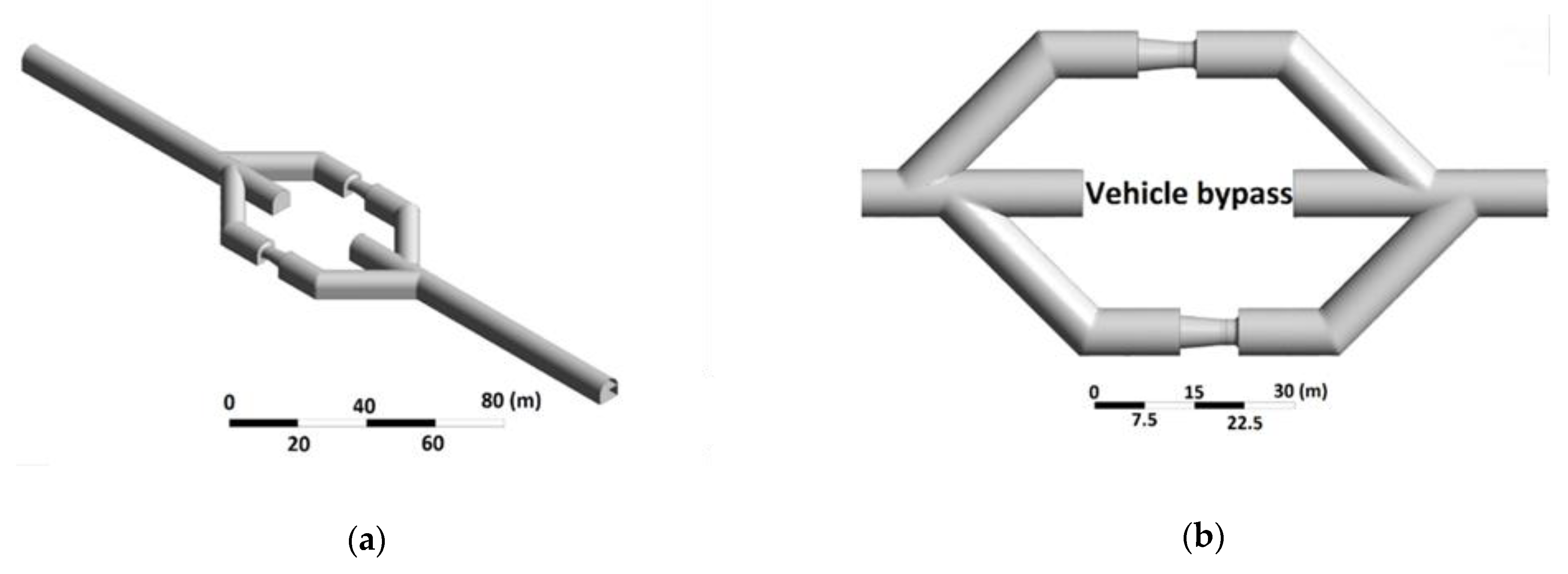
Figure 4.
Run around parallel fan station 3D model (a) isometric view; (b) plan view.
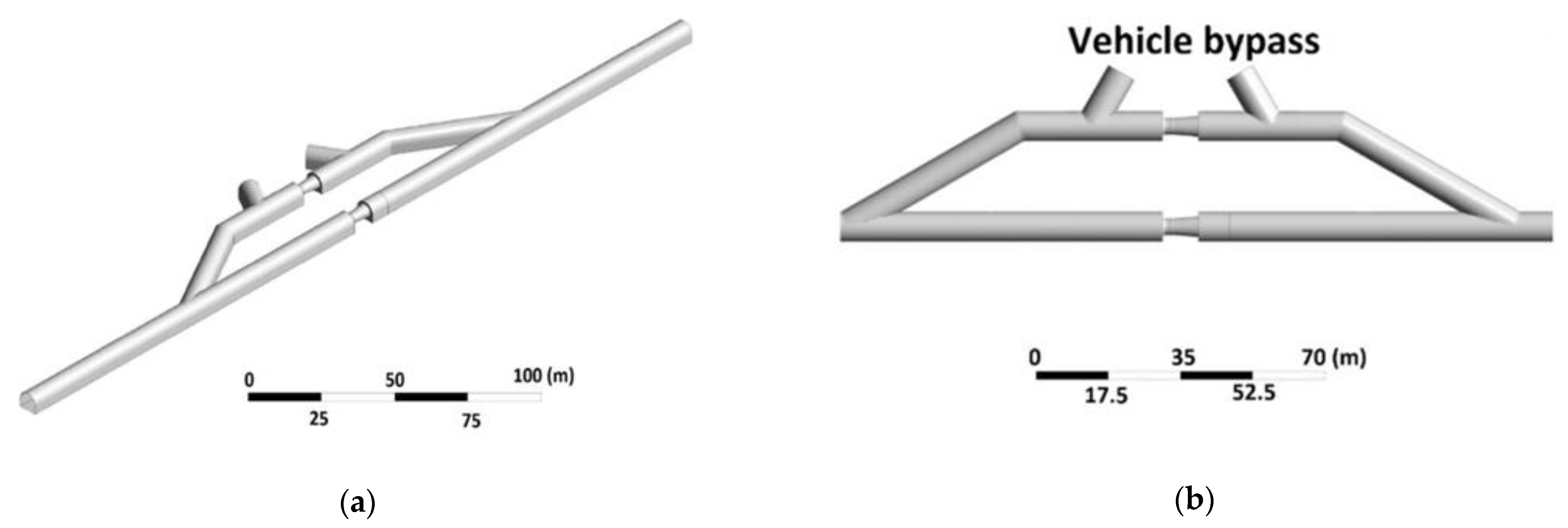
Figure 5.
Boundary condition location.

Figure 6.
Static pressure measurement for a fan in booster mode.

Figure 7.
Fan naming according to airflow direction, “a” top fan and “b” bottom fan.

Figure 8.
Mesh details in fan zone (A) side view; (B) 3D view.

Figure 9.
(a) Ventilation station operational point comparison for different geometries and resistances; (b) individual fans operational points comparison for different geometries and resistances.
Figure 9.
(a) Ventilation station operational point comparison for different geometries and resistances; (b) individual fans operational points comparison for different geometries and resistances.
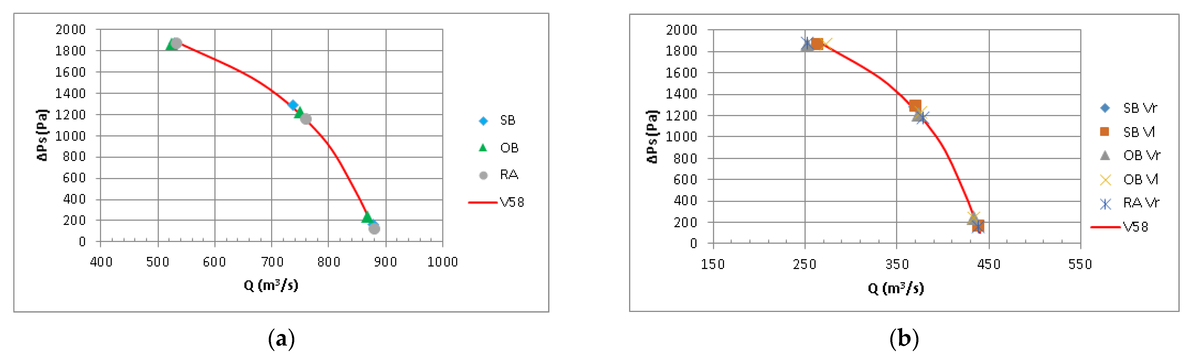
Figure 10.
Close-up of operational points for the analyzed fans (B.C. Kentry = 0, Koutlet = 6.5).
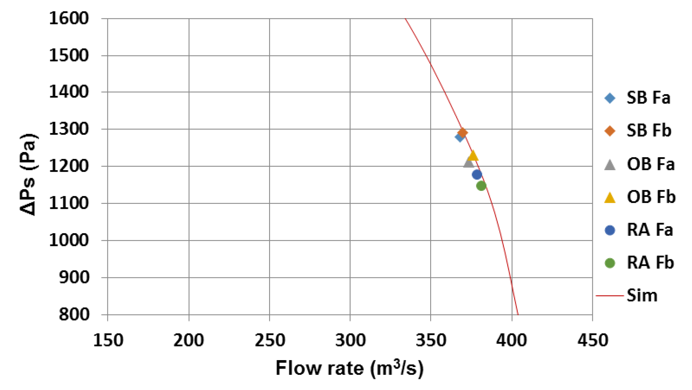
Figure 11.
System resistance curve comparison based on station geometry (A) complete fan curve; (B) operational points.
Figure 11.
System resistance curve comparison based on station geometry (A) complete fan curve; (B) operational points.
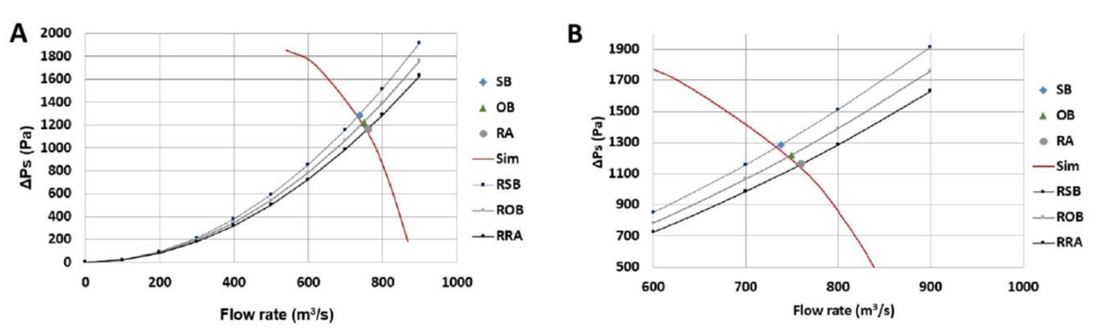
Figure 12.
Velocity vector (colored by velocity magnitude) of individual fans (left a and right b) for symmetrical branches (SB, top), overlapped branches (OB, middle), and run around (RA, bottom).
Figure 12.
Velocity vector (colored by velocity magnitude) of individual fans (left a and right b) for symmetrical branches (SB, top), overlapped branches (OB, middle), and run around (RA, bottom).

Figure 13.
Velocity vector (colored by velocity magnitude) of individual fans for symmetrical branches (SB, top), overlapped branches (OB, middle), and run around (RA, bottom). Left inlet (i) and right outlet (o).
Figure 13.
Velocity vector (colored by velocity magnitude) of individual fans for symmetrical branches (SB, top), overlapped branches (OB, middle), and run around (RA, bottom). Left inlet (i) and right outlet (o).
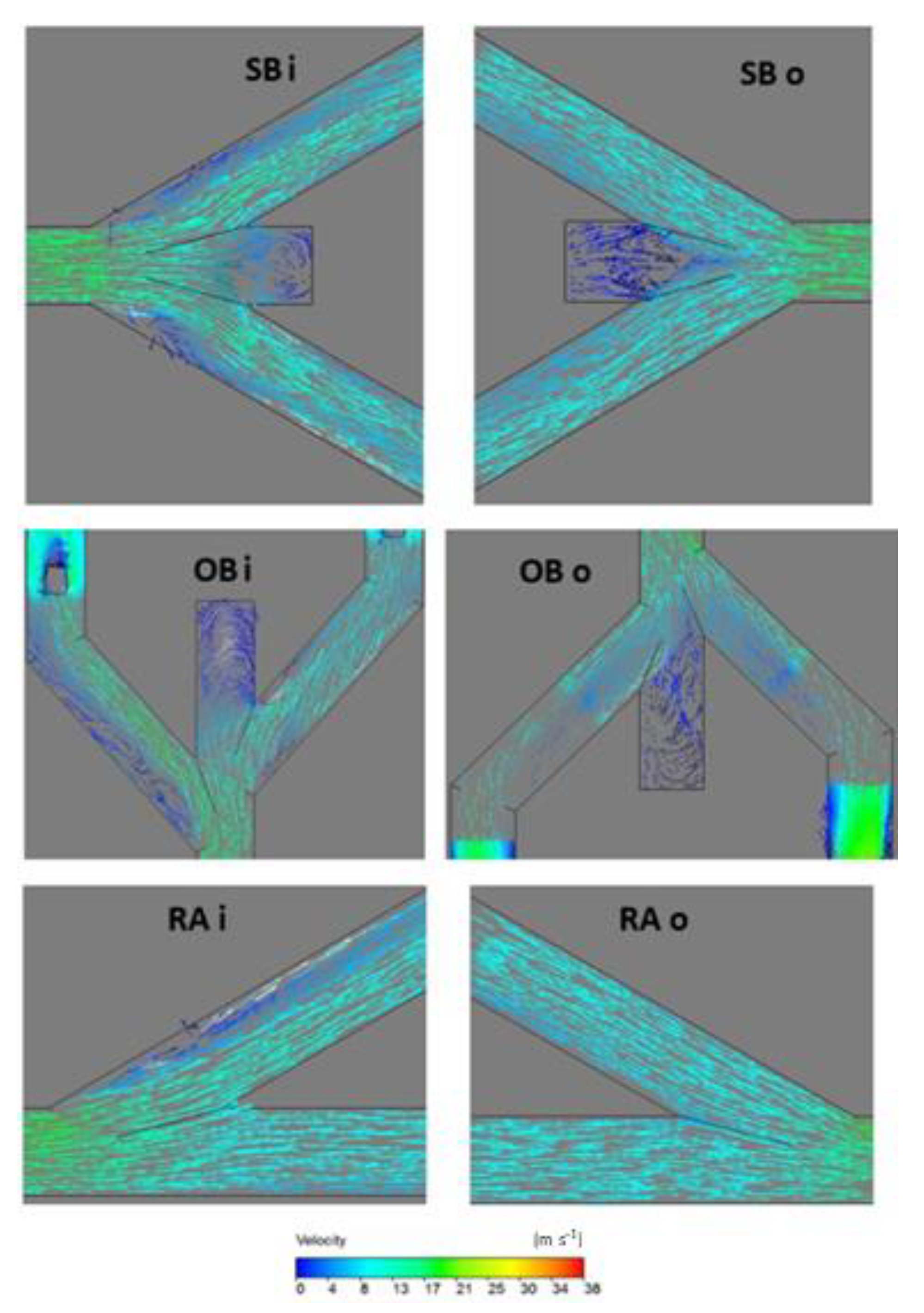
Figure 14.
Velocity vector of individual fans (left and right) for symmetrical branches (SB, top), overlapped branches (OB, middle), and run around (RA, bottom).
Figure 14.
Velocity vector of individual fans (left and right) for symmetrical branches (SB, top), overlapped branches (OB, middle), and run around (RA, bottom).
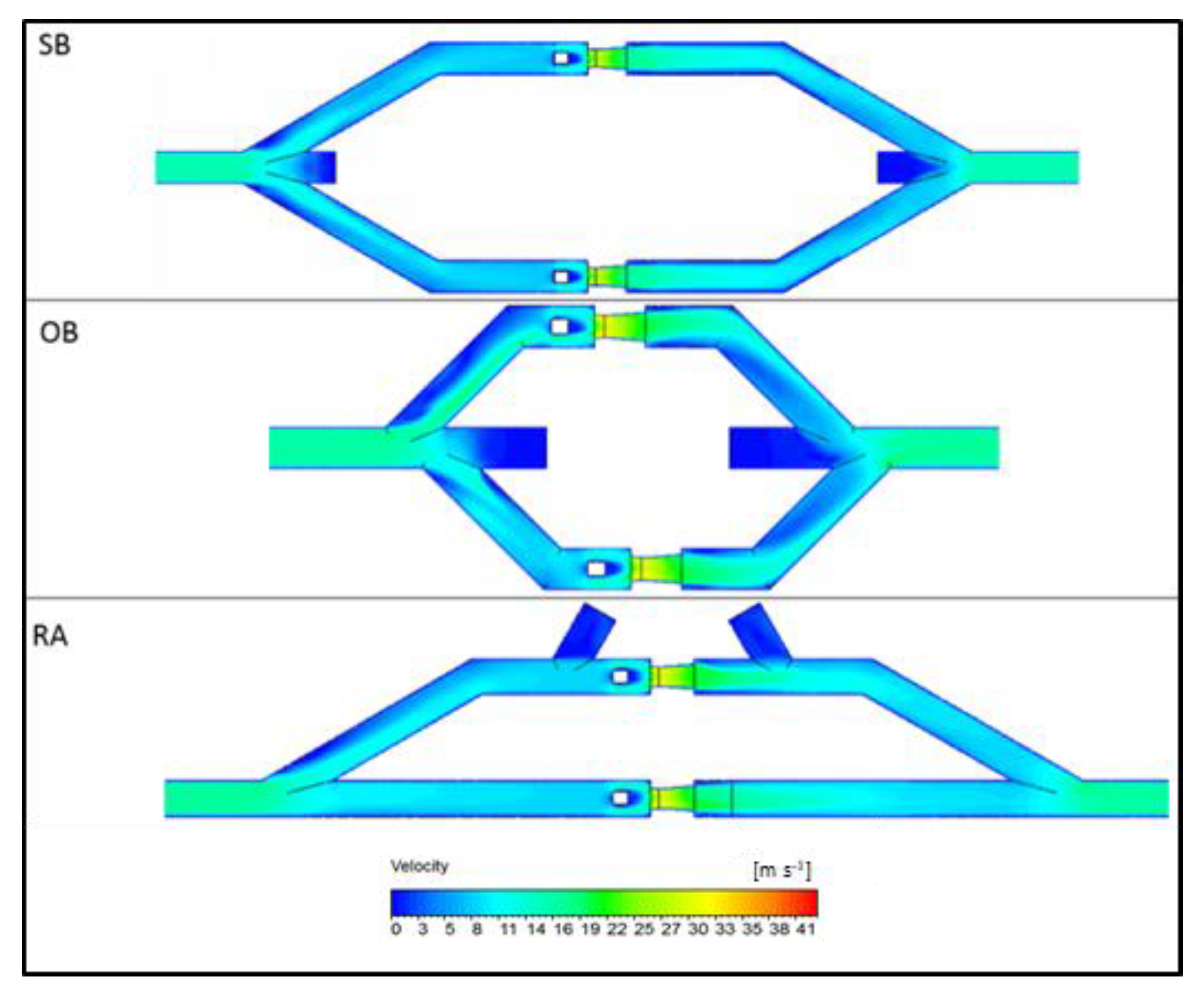
Figure 15.
Static pressure vector of individual fans (left and right) for symmetrical branches (SB, top), overlapped branches (OB, middle), and run around (RA, bottom).
Figure 15.
Static pressure vector of individual fans (left and right) for symmetrical branches (SB, top), overlapped branches (OB, middle), and run around (RA, bottom).
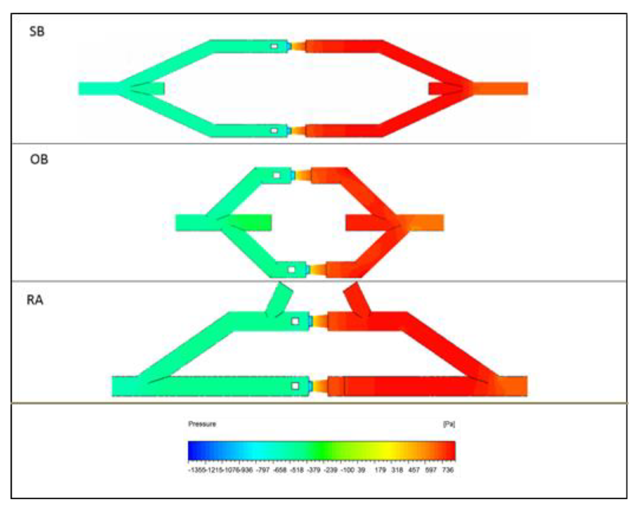
Figure 16.
Velocity vectors on run around fan station, with an adjusted velocity scale to appreciate differences of velocities in the stream before fans.
Figure 16.
Velocity vectors on run around fan station, with an adjusted velocity scale to appreciate differences of velocities in the stream before fans.


Table 1.
Loss coefficients for fan ventilation stations.
| Kentry | Koutlet |
|---|---|
| 7.5 | 15 |
| 7.5 | 7 |
| 0 | 6.5 |
| 0 | 3 |
| 0 | 0 |
Table 2.
Operational points for studied fan ventilation station geometries.
| Kinlet | Koutlet | QFanA (m3/s) | Ps-FanA (Pa) | QFanB (m3/s) | Ps-FanB (Pa) | QTotal (m3/s) | Ps-Total (Pa) | Hydraulic Power (kW) |
|---|---|---|---|---|---|---|---|---|
| Symmetrical branches (SB) | ||||||||
| 7.5 | 15 | 266 | 1871 | 264 | 1873 | 529 | 1872 | 991 |
| 7.5 | 7 | 309 | 1668 | 310 | 1675 | 619 | 1672 | 1034 |
| 0 | 6.5 | 368 | 1280 | 370 | 1291 | 738 | 1285 | 949 |
| 0 | 3 | 411 | 720 | 412 | 731 | 823 | 726 | 597 |
| 0 | 0 | 439 | 156 | 439 | 166 | 878 | 161 | 141 |
| Overlapped branches (OB) | ||||||||
| 7.5 | 15 | 252 | 1858 | 273 | 1874 | 525 | 1866 | 980 |
| 7.5 | 7 | 305 | 1667 | 308 | 1684 | 613 | 1676 | 1027 |
| 0 | 6.5 | 374 | 1212 | 376 | 1231 | 750 | 1221 | 916 |
| 0 | 3 | 405 | 760 | 408 | 787 | 814 | 773 | 629 |
| 0 | 0 | 434 | 239 | 418 | 242 | 851 | 241 | 205 |
| Run around (RA) | ||||||||
| 7.5 | 15 | 279 | 1856 | 252 | 1880 | 532 | 1868 | 993 |
| 7.5 | 7 | 313 | 1644 | 307 | 1674 | 620 | 1659 | 1029 |
| 0 | 6.5 | 381 | 1148 | 379 | 1177 | 760 | 1162 | 883 |
| 0 | 3 | 415 | 673 | 411 | 726 | 826 | 699 | 577 |
| 0 | 0 | 441 | 98 | 439 | 156 | 880 | 127 | 112 |
Table 3.
Ventilation system resistance operational points for studied fan ventilation station geometries.
Table 3.
Ventilation system resistance operational points for studied fan ventilation station geometries.
| K | SB | OB | RA | |||||||
|---|---|---|---|---|---|---|---|---|---|---|
| Kinlet | Koutlet | Q (m3/s) | Ps (Pa) | R (kg s2/m8) | Q (m3/s) | Ps (Pa) | R (kg s2/m8) | Q (m3/s) | Ps (Pa) | R (kg s2/m8) |
| 7.5 | 15 | 529 | 1872 | 0.00668 | 525 | 1866 | 0.00677 | 532 | 1868 | 0.00661 |
| 0 | 6.5 | 738 | 1285 | 0.00236 | 750 | 1221 | 0.00217 | 760 | 1162 | 0.00201 |
| 0 | 0 | 878 | 161 | 0.00021 | 868 | 241 | 0.00032 | 880 | 127 | 0.00016 |
Table 4.
Ventilation station power consumption.
| K | Hydraulic Power (kW) | ∆ (kW) | |||||
|---|---|---|---|---|---|---|---|
| Kinlet | Koutlet | SB | OB | RA | ∆(RA − SB) | ∆(RA − OB) | ∆(SB − OB) |
| 7.5 | 15 | 991 | 980 | 993 | 2 | 14 | 11 |
| 0 | 6.5 | 949 | 916 | 883 | −65 | −32 | 33 |
| 0 | 0 | 141 | 209 | 112 | −30 | −97 | −68 |
Table 5.
Annual ventilation station energy consumption.
| K | Year Consumption (MWh/year) | ∆ (MWh) | |||||
|---|---|---|---|---|---|---|---|
| Kinlet | Koutlet | SB | OB | RA | ∆(RA − SB) | ∆(RA − OB) | ∆(SB − OB) |
| 7.5 | 15 | 8246.1 | 8151.9 | 8265.3 | 19.2 | 113.5 | 94.3 |
| 0 | 6.5 | 7894.3 | 7618.9 | 7350.4 | −543.9 | −268.5 | 275.4 |
| 0 | 0 | 1175.2 | 1737.7 | 928.5 | −246.7 | −809.2 | −562.5 |
Table 6.
Net Present Value (NPV) comparison of parallel fan station costs over 20 years.
| Year | Total Cost (kUSD) | % Difference (RA over OB) | ||
|---|---|---|---|---|
| SB | OB | RA | ||
| 1 | 4457.4 | 3522.2 | 4134.1 | 15% |
| 2 | 5473.0 | 4502.6 | 5079.1 | 11% |
| 3 | 6413.4 | 5410.3 | 5954.1 | 9% |
| 4 | 7284.2 | 6250.7 | 6764.3 | 8% |
| 5 | 8090.4 | 7028.9 | 7514.5 | 6% |
| 6 | 8836.9 | 7749.5 | 8209.1 | 6% |
| 7 | 9528.2 | 8416.7 | 8852.2 | 5% |
| 8 | 10,168.2 | 9034.5 | 9447.7 | 4% |
| 9 | 10,760.8 | 9606.5 | 9999.1 | 4% |
| 10 | 11,309.5 | 10,136.1 | 10,509.7 | 4% |
| 11 | 11,817.6 | 10,626.5 | 10,982.4 | 3% |
| 12 | 12,288.0 | 11,080.6 | 11,420.1 | 3% |
| 13 | 12,723.6 | 11,501.0 | 11,825.4 | 3% |
| 14 | 13,126.9 | 11,890.3 | 12,200.7 | 3% |
| 15 | 13,500.4 | 12,250.8 | 12,548.2 | 2% |
| 16 | 13,846.2 | 12,584.5 | 12,869.9 | 2% |
| 17 | 14,166.3 | 12,893.6 | 13,167.8 | 2% |
| 18 | 14,462.8 | 13,179.7 | 13,443.7 | 2% |
| 19 | 14,737.3 | 13,444.7 | 13,699.1 | 2% |
| 20 | 14,991.4 | 13,690.0 | 13,935.5 | 2% |
Table 7.
Number of years for payback of RA geometry over OB geometry according to energy and development cost analysis.
Table 7.
Number of years for payback of RA geometry over OB geometry according to energy and development cost analysis.
| Development Cost of 7.2 m × 7.2 m Cross Section (USD/m) | ||||||
|---|---|---|---|---|---|---|
| Energy Cost (USD/kWh) | 3500 | 4000 | 4500 | 5000 | 5500 | 6000 |
| 75 | - | - | - | - | - | - |
| 100 | - | - | - | - | - | - |
| 125 | 22 | 35 | - | - | - | - |
| 150 | 15 | 20 | 27 | 47 | - | - |
| 175 | 12 | 15 | 18 | 24 | 33 | - |
| 200 | 10 | 12 | 14 | 17 | 21 | 27 |
| 225 | 8 | 10 | 12 | 14 | 17 | 20 |
| 250 | 7 | 9 | 10 | 12 | 14 | 16 |
Publisher’s Note: MDPI stays neutral with regard to jurisdictional claims in published maps and institutional affiliations. |
© 2021 by the authors. Licensee MDPI, Basel, Switzerland. This article is an open access article distributed under the terms and conditions of the Creative Commons Attribution (CC BY) license (https://creativecommons.org/licenses/by/4.0/).
Share and Cite
MDPI and ACS Style
Hurtado, J.P.; Reyes, G.; Vargas, J.P.; Acuña, E. A Computational Fluid Dynamic Study of Developed Parallel Stations for Primary Fans. Processes 2021, 9, 1607. https://doi.org/10.3390/pr9091607
AMA Style
Hurtado JP, Reyes G, Vargas JP, Acuña E. A Computational Fluid Dynamic Study of Developed Parallel Stations for Primary Fans. Processes. 2021; 9(9):1607. https://doi.org/10.3390/pr9091607
Chicago/Turabian StyleHurtado, Juan Pablo, Gabriel Reyes, Juan Pablo Vargas, and Enrique Acuña. 2021. "A Computational Fluid Dynamic Study of Developed Parallel Stations for Primary Fans" Processes 9, no. 9: 1607. https://doi.org/10.3390/pr9091607
Note that from the first issue of 2016, this journal uses article numbers instead of page numbers. See further details here.