Effects of Flow Baffles on Flow Profile, Pressure Drop and Classification Performance in Classifiers

Abstract

This paper presents a study of the use of flow baffles inside a centrifugal air classifier. An air classifier belongs to the most widely used classification devices in mills in the mineral industry, which is why there is a great interest in optimizing the process flow and pressure loss. Using Computational Fluid Dynamics (CFD), the flow profile in a classifier without and with flow baffles is systematically compared. In the simulations, turbulence effects are modeled with the realizable k–ε model, and the Multiple Reference Frame approach (MRF) is used to represent the rotation of the classifier wheel. The discrete phase model is used to predict the collection efficiency. The effects on the pressure loss and the classification efficiency of the classifier are considered for two operating conditions. In addition, a comparison with experimental data is performed. Firstly, the simulations and experiments show good agreement. Furthermore, the investigations show that the use of flow baffles is suitable for optimizing the flow behavior in the classifier, especially in reducing the pressure loss and therefore energy costs. Moreover, the flow baffles have an impact on the classification performance. The impact depends on the operation conditions, especially the classifier speed. At low classifier speeds, the classifier without flow baffles separates more efficiently; as the speed increases, the classification performance of the classifier with flow baffles improves.

1. Introduction

The air classification of gas–particle flows is an essential step in mineral, pharmaceutical, food, coal and cement industries [1,2,3,4,5]. Especially for high product flows and fine target products, centrifugal classifiers are commonly installed. The general function of a classifier is to separate particles into coarse and fine particle fractions. This is achieved by rotating the classifier wheel, whereby centrifugal forces act against the drag forces, and particles are classified according to size. Coarse particles are thus rejected at the outer edge of the classifier wheel, while finer particles are transported inwards with the air to the product outlet [6]. In order to reduce the process stages in a system, grinding and classification usually take place in a single apparatus. This enables continuous operation, since particles that are too coarse are returned directly to the grinding process after being rejected at the classifier. The high mass flows cause high operational energy costs. Therefore, interest in optimizing the process is of great importance. For this purpose, several experimental and numerical studies have been carried out in the past.

A detailed description of the flow profile in the classifier was first given by Toneva et al. [7]. According to this, the flow profile shows three characteristic regions. The first region is located between the classifier blades. Here, the flow forms a forced vortex with high tangential velocity. Depending on the speed of the classifier, a dead zone is created, which decreases the classification performance of the apparatus. Between the classifier blades and the center of the classifier, two other regions appear with opposite physical behaviors. At the inner edge of the classifier blades lies the second region, where the tangential velocity increases with decreasing radius. In the center of the classifier is the third region, which is in contrast to the second region. This has similar characteristics to a forced vortex, and the tangential velocity decreases rapidly. The size of the individual regions depends on the process parameters and the design of the classifier. Many researchers have now confirmed Toneva’s studies [8,9]. For example, Stender et al. [8] were able to gain optical access to the processes in the classifier. By using a camera, the real particle movement during classification was observed for the first time. In recent years, research has mainly focused on the optimization of geometric aspects of the classifier blades or the differences between vertical or horizontal classifiers [10,11,12,13,14]. For this purpose, CFD was primarily chosen, as it is a cost-effective and time-saving tool and provides a sufficiently accurate representation of characteristic values such as pressure drop and classification efficiency [15,16,17]. Nevertheless, the inner region of the classifier, characterized by Toneva as the second and third regions, has always been neglected during optimization. This zone, however, requires special attention, since high velocity and pressure changes occur in this region. The potential to optimize the flow profile and reduce pressure losses shows studies of Guizani et al. [18]. During the investigations, the fine material outlet of a classifier was changed, which significantly reduced the pressure loss.

This work investigates the effect of flow baffles inside the classifier on the flow profile, pressure drop and classification efficiency. For this purpose, different classifier geometry are simulated. The geometries are different inside the classifier, namely no and twelve baffles are integrated. The baffles are attached to the rotor so that they have the same speed as the classifier. The speed of the classifier is varied, as the performance of the baffles also depends on it. The Multiple Reference Frame model (MRF) represents the rotation of the classifier. To evaluate the classification efficiency, the discrete phase model (DPM) is implemented to estimate particle trajectories. In addition, experimental tests for both types of classifiers are performed. Finally, this works compares two operating conditions for experimental and simulation results for validation.

2. Materials and Methods

2.1. Experimental Set-Up

A schematic view of the complete process is shown in Figure 1. In the process, air is recirculated in the system with a fan. To prevent water from accumulating, a part of the air is exchanged. The main part of the process is the mill and the classifier. The mill itself consists of four rollers held in a fixed position on a rotating bowl. The mill and the classifier are also illustrated in Figure 1. Air enters the mill from below via a nozzle ring and transports comminuted particles thrown off by the rotating bowl to the top. The classifier is above the mill. A first classification takes place in the transport section between the mill and the classifier, since very coarse particles do not reach the top due to gravity. Finer particles pass with the air through the static blades and reach the classifier. The rotating classifier rejects coarser particle due to centrifugal forces, while finer particles pass inside with the air and reach the fines. The coarse particles move in a circular path around the classifier and slowly sediment to the bottom, where the particles are fed again into the grinding process. In addition, solid material is fed onto the grinding bowl via a screw conveyor. A cyclone separates the fine particles after the classifier from the air, where a sample of the fine product is taken and analyzed. The particle size distribution of the sample is measured by laser diffraction with a Mastersizer 2000 provided by Malvern Panalytical. Measuring points for measuring pressure drop are set up in front of the static guide vanes and after the classifier. Static pressure is measured with a barometer that uses a liquid column. The static pressure versus atmospheric pressure is determined for the two measurement points, and then the difference is formed. Water is used as the liquid. The left-hand side of Figure 1 illustrates the measuring points of the pressure drop measurement.

The fluctuations of the measurement were about 0.2 mbar, i.e., negligibly small compared to pressure losses of 30 mbar. This was due to the uniform velocities in these geometric sections. Due to the low fluctuations, the measured values could be used for comparison with the simulations. It was expected that the influence of the baffles on the performance of the classifier would depend on the operating conditions, especially the classifier speed. Therefore, the classifier was operated without and with 12 baffles at two different operating conditions. The flow baffles were located inside the classifier and were attached to the classifier and shaft. They can also be seen in Figure 1. The operating conditions differed in terms of classifier speed, rotating bowl speed, solid feed, volume flow and processed material. A detailed description of the operating conditions is shown in

Table 1. Characteristic sizes of materials, fluid and classifier for first operating conditions.

	Name	Unit	Size
Material 1	Solid feed	t/h	20
“Pozzolan A”	density	kg/m3	2540
Fluid	Temperature	°C	100
“Air”	Volume flow	m3/h	63,000
Classifier	Speed	rpm	135

and

Table 2. Characteristic sizes of materials, fluid and classifier for second operating conditions.

	Name	Unit	Size
Material 2	Solid feed	t/h	5
“Pozzolan B”	density	kg/m3	2610
Fluid	Temperature	°C	100
“Air”	Volume flow	m3/h	43,500
Classifier	Speed	rpm	500

.

The classifier has a diameter of 1.6 m and consist of 48 blades. The static blades have an outer diameter of 2.1 m and comprise 60 blades. The mill has 4 rollers. The grinding bowl diameter is 1.85 m. The focus of the investigations was on the classifier; therefore, this study neglected the influence of the mill, and no further information on the mill will be provided.

2.2. Numerical Set-Up

The basic task of the numerical investigations is the impact of baffles within the classifier on the flow field, pressure drop and thus on grade efficiency of the apparatus. The high complexity and size of the classifier together with the high number of particles requires certain assumptions due to the high computational effort. Firstly, the flow in a classifier is typically a high swirling flow due to the rotating parts in the classifier. This symbolizes the Reynolds number, which is around 9.5 × 10⁵ in the classifier outlet area and characterize the flow as turbulent. The realizable k–ε, an approach using the Reynolds Averaged Navier–Stokes Equations (RANS), serves as a model to predict the turbulent character of the flow regime. The realizable k–ε is appropriate for fully turbulent rotating flows in which high strain rate and curvature of streamline occurs [11,15]. Secondly, the rotation of the classifier needs special attention. The Multiple Reference Frame (MRF) allows one to simulate the interaction between moving and stationary parts. The MRF Model treats flow differently depending on the region. The rotating sections are frozen in position, and the model solves the Navier–Stokes equation, including the centrifugal and Coriolis forces. Rotating walls rotate as a rigid body. Standing walls receive the no slip condition. The MRF model does not represent nonstationary effects due to rotation. Nevertheless, the MRF model is suitable for the simulation of a classifier due to its advantages of being robust and that there is no tight coupling between moving parts and stationary parts [7,18]. Furthermore, air is assumed to be an incompressible, isothermal, Newtonian fluid.

For adequately describing the dispersed phase, the Discrete Phase Model (DPM) is used. The particle laden flow is only studied in the upper part of the machine in the area of the classifier, which is why the particles are abandoned above the mill. Particles which are deposited at the classifier are detected as well as particles falling down to the mill. The fine particles passing through the classifier are also detected. This enables the creation of classification efficiency curves for the investigated classifier. In the experiments, only the fines were available for analysis. A discrete number of particles represents the solid phase. Particles are tracked though the air flow. Particle–particle interaction as well as particle comminution or accumulation are considered. The trajectory of a particle is given by the integration of the momentum balance of a particle. The equations of motion for an individual particle in rotating region can be written as

$$\frac{\mathsf{\pi } x^3}{6}{\rho }_P\frac{d{\overrightarrow{u}}_P}{dt}=\frac{\mathsf{\pi }}{8} C_D {\rho }_F x^2 |{\overrightarrow{v}}_{rel}| {\overrightarrow{v}}_{rel} + \frac{\mathsf{\pi } x^3}{6} {\rho }_P \overrightarrow{g} + m_P(-2\overrightarrow{\Omega }\times {\overrightarrow{u}}_P) + m_P(-\overrightarrow{\Omega }\times \overrightarrow{\Omega }\times \overrightarrow{r})$$

(1)

The terms on the right-hand side represents the drag force, the gravity force, the Coriolis force and centrifugal force. Coriolis and centrifugal forces result from the rotation of the classifier. $x$ is the diameter of a particle, ${\overrightarrow{u}}_P$ the particle velocity, ${\rho }_P$ the density of the particle, $C_D$ the drag coefficient, ${\rho }_F$ the density of the air and ${\overrightarrow{v}}_{rel}$ the relative velocity between the fluid and the particle. $\overrightarrow{g}$ is the gravity vector, $m_P$ the mass of a particle, $\Omega$ the angular velocity and $\overrightarrow{r}$ the radial position vector. Other forces such as Saffmann, virtual mass force and Basset term can be neglected. The drag model uses an assumption of solid spheres:

$${ C}_D=\{\begin{array}{c}24 \left(1+\frac{1}{6}{Re}_P{}^{\frac{2}{3}}\right) Re\le 1000 \\ 0.424 {Re}_P Re>1000 \end{array}$$

(2)

The particle Reynolds number ${Re}_P$ is

$${Re}_P= \frac{{ \rho }_F x v_{rel}}{{\mu }_F}$$

(3)

where ${\mu }_F$ is the kinematic viscosity of the air. The particle Reynolds number is in the range of 0.1 to 5 in the classifier outlet area. Moreover, a stochastic dispersion model considers the effect of turbulence during the particle tracking. Therefore, the velocity fluctuation is perturbed in a random direction with a Gaussian random number. Particle–wall collisions are elastic and specular. Additionally, the approach neglects the influence of particle rotation.

In order to investigate the classification efficiency of the classifier, 10⁷ spherical particles were tracked in the simulation. The feed zone was above the mill with an initial velocity of 4 m/s. The air outlet and mill area were escape boundaries, which means that the calculation stopped once particles reached them. The solid loading and the volume flow was assumed to be the same as in the experiments. In the experiments, the material was comminuted in the mill, which is why the particle distribution reaching the classifier was not known. Therefore, a fictive particle distribution in the particle size range from 1 to 500 µm was specified in the simulation. The continuous operation of the plant and the impossibility to simulate the comminution process did not allow for a direct comparison between experimental and numerical results. Only a quantitative comparison took place in the results.

All simulations were performed with the software environment OpenFoam-6. A solver was adapted according to the equation described above, and two-way coupling between the continuous and dispersed phase was included. Standard no-slip boundaries were applied to all walls, including the classifier. As boundary conditions, a relative total pressure of 0 Pa was specified at the outlet of the classifier. Furthermore, the same volume flow as used in experiments was defined at the mill inlet. An overview of the selected boundary conditions is shown in

Table 3. Boundary conditions.

	Inlet	Outlet	Wall
Velocity	Fixed value	Zero gradient	No slip
Pressure	Zero gradient	Total pressure 0 Pa	Zero gradient

.

The geometry used in the simulation was a faithful representation of the original geometry, except for minor details such as welds, minor edges or closed volumes that are not of practical importance to the flows and were omitted to limit model complexity. Nonetheless, due to its complexity, the two grids, without and with baffles, consisted of around 15 million elements. The grids were composed of an unstructured, hexahedral mesh with prism layers created by the OpenFOAM meshing tool snappyHexMesh. The value of y+ was for all walls between 30 and 300 and thus fit the requirements of the turbulence model. The mesh quality for both grids was as follow: maximum skewness of 2.8, non-orthogonality of less than 66° and an aspect ratio of less than 17. An overview of the complete grid and the classifier with baffles is illustrates in Figure 2.

Three different meshes were generated.

Table 4. Comparison of pressure loss for three grids between simulation and experiment at second operation conditions in Table 2 and classifier without baffles.

Grid	Number of Elements	Pressure Loss in Simulation in Pa	Standard Deviation to Experiment in %
Coarse grid	6 m	2421	27.1
Medium grid	15 m	2976	10.4
Fine grid	24 m	3012	9.3

compares the pressure loss from the simulation with experimental data for the three grids. The comparison is for the second operation conditions. The standard deviation was calculated to pressure loss in experiment for all grids.

In order to investigate mesh sensitivity, further values were studied. Firstly, the average radial and tangential velocity between the classifier blades were compared. Secondly, we investigated the velocities in the transport section between mill and classifier. Thirdly, the resulting overall pressure drop in the classifier and mill was plotted against experimental data. This last comparison also determined the accuracy of the numerical model. The comparison of measured and simulated values is shown for the two operating conditions for the classifier without blades in

Table 5. Comparison of pressure loss in Pa in experiment and simulation for both classifier at first operation conditions.

	Without Baffles	With Baffles	Standard Deviation in %
Experiment	2405	2098	12.6
Simulation	2120	1875	11.6

and

Table 6. Comparison of pressure loss in Pa in experiment and simulation for both classifier at second operation conditions.

	Without Baffles	With Baffles	Standard Deviation in %
Experiment	3321	2460	25.9
Simulation	2976	2189	26.4

.

The results show that the pressure loss was slightly underestimated in the simulation. The standard deviation was around 10%, which is probably due to fact that turbulence effects were modelled with the realizable k–ε approach. However, a complete resolution of turbulence effects is too time consuming.

3. Results

The time-averaged velocity distributions inside the mill and classifier with no and twelve baffles were investigated, and the CFD results for the second operating condition are reported in Figure 3. The second operation condition had a higher classifier speed of 500 rpm, and the outer edge of the classifier rotated at about 42 m/s. Since only the inner area of the classifier was changed, the flow profiles in the grinding area did not differ for both cases. The air was guided through the nozzle ring after the inlet, causing the air in the outer area to rise upwards to the classifier. The highest velocities occurred between the classifier blades and the inner edge of the classifier cage. In the center of the classifier, the velocity decreased. In general, the flow profiles for both geometries were very similar; differences only became apparent when taking a closer look within the classifier wheel.

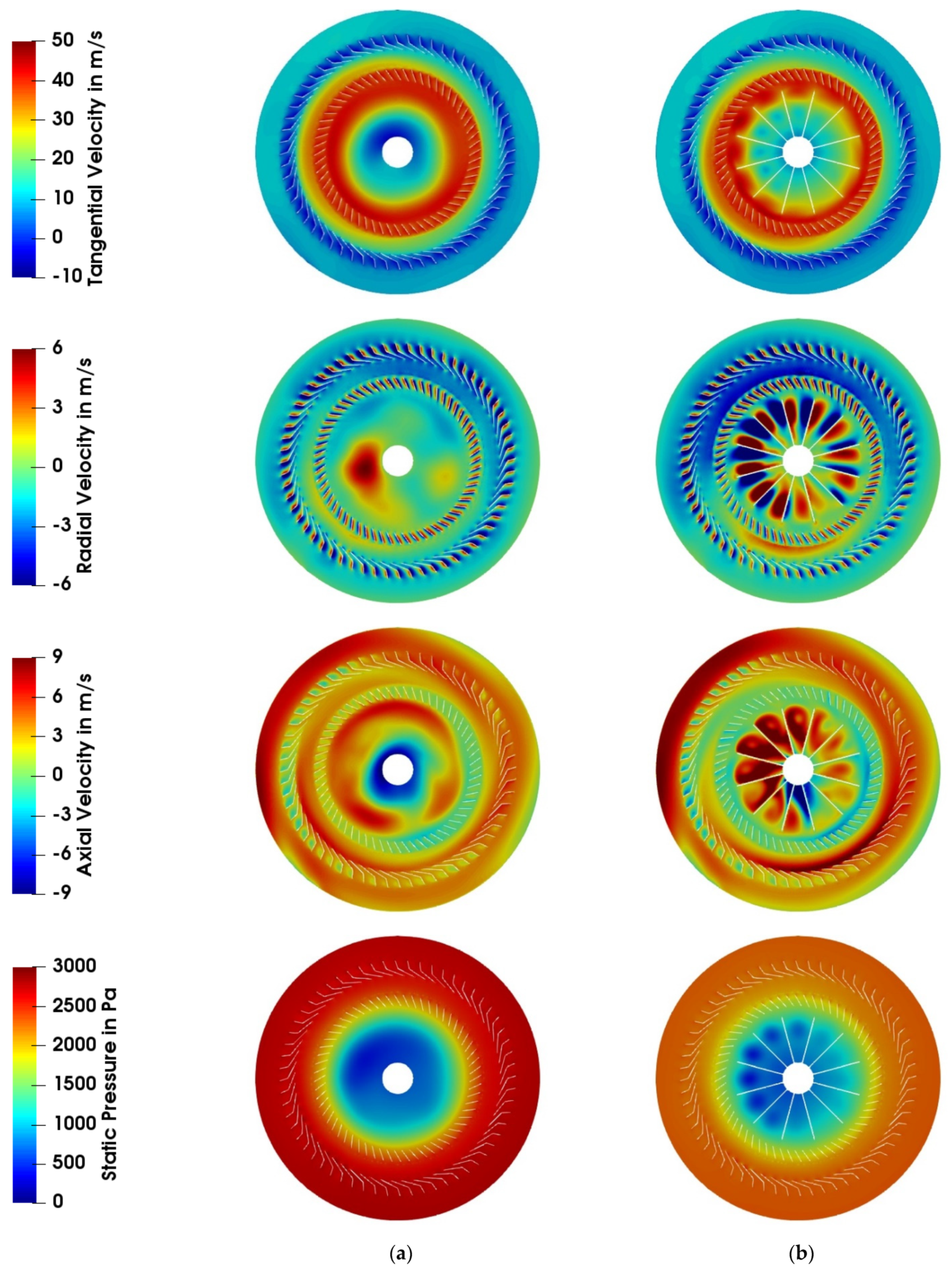
Therefore, Figure 4 shows the velocity profiles for the tangential, axial and radial component in an axial section through the classifier and the static blades. Figure 4 also shows the resulting pressure drop for investigated geometries. Without baffles inside the classifier, the flow profile with the three regions described by Toneva [7] was formed. The tangential velocity reached the maximum velocity on the inner edge of the classifier cage.

Moreover, the forced vortex inside the classifier was strongly impressed, and the tangential velocity dropped sharply with a lower radius. This vortex led to a huge reduction in static pressure. In addition, the flow formed a vortex between the classifier blades. Behind the trailing blades, the radial velocity was shown by blue zones, indicating a radial velocity outwards, in front of the leading blade the air flows inwards, which was indicated by red velocity. Positive axial velocities occurred mainly outside of the static blades, between the static blades and the classifier, and inside the classifier. In the center of the classifier, negative axial velocities were present. The flow baffles changed the typical flow profile, which resulted in a slight reduction of the maximum tangential velocity. However, negative tangential velocity inside the classifier and negative axial velocities could be minimized or avoided. This significantly reduced the pressure loss in the classifier with baffles.

A qualitative indication of the reduction in pressure drop is provided by Table 4 and Table 5. There, the pressure loss in the experiment and simulation is presented for both classifier and operation conditions. The tables show firstly that, as already mentioned above, the pressure drop in the simulation was always lower than in the experiment, and secondly, that the pressure drop for both operating conditions could be significantly reduced by using flow baffles. For the first operating conditions at low classifier speed and high solid loading and volume rate, the reduction was around 12%; at the second operating condition at higher classifier speed and lower solid loading and lower volume flow, the pressure reduction was around 26%. Thus, thirdly, the tables show that the reduction in pressure drop depends on the operating conditions. The higher the classifier speed and the lower the volume flow, the greater the effect of the baffles. Fourthly, the simulation predicted very well the pressure loss reduction.

In addition to pressure loss, classification efficiency is also an important parameter to evaluate the classifier performance. In the simulations, particles in the size range of 1–500 µm were tracked. The number of particles varied in the range of 100,000 and 1,000,000. The particle distribution in the feed as well as the number of tracked particles had only a minor influence on the classification efficiency in the classifier. Since the particle distribution reaching the classifier in the experiments after grinding is unknown, an exact validation of experiment and simulation was not possible. Particles were fed between the classifier and the mill in the simulation, and their pathlines were recorded through the classifier. The end of tracking was reached when a particle left the classifier through the air exit or was rejected by the classifier and sediments towards the mill rollers. As an example, two different particle trajectories for a coarse particle of 50 µm and a fine particle of 10 µm for the classifier with twelve baffles and the second operating condition are shown in Figure 5.

The particle trajectories refer to the absolute motion of a particle, which is why they also move through rotating walls such as classifier blades and baffles in Figure 5. As expected, the fine particle enters the fine material while the coarse particle is rejected several times on the classifier. The particle trajectories can be used to calculate the grade efficiency T(x), which describes what fraction of the feed is in the coarse material after classification. Therefore, the grade efficiency results in

$$T(x)= \frac{m_C}{m_{Feed}}\frac{q_{3,C}\left(x\right)}{q_{3,Feed}\left(x\right)}100\%$$

(4)

where $m_C$ is the coarse material mass, $m_{Feed}$ is the feed material mass, $q_{3,C}$ is the particle density distribution of the coarse material and $q_{3,Feed}$ is particle density distribution of the feed. Figure 6 shows the results of the classification efficiency curves for both operating conditions and classifier types of the simulation. At the second operating condition, finer separation is achieved because the speed of the classifier is much higher and therefore greater centrifugal forces act on the particles.

It is also noticeable that at low classifier wheel speed, i.e., the first operating condition, the classifier without baffles separates more effectively, while at high speed the grade efficiency of the two separators is almost the same. Furthermore, the fish-hook effect is more pronounced in the classifier without baffles than in the classifier with baffles at the second operating point. In the experiments, only the fines were available for analysis. Therefore, two values were measured to evaluate the grade efficiency in the experiments. Firstly, the Blaine value was used, which is a standardized measure for the degree of fineness of a material and is determined via the specific surface area [19]. The higher the Blaine value, the finer the material and thus the better the separation of the classifier. Secondly, the residue on the sieve in µm was compared between classifier with and without baffles.

Table 7. Blaine value and residue on sieve in experiment at first operating condition.

	Without Baffles	With Baffles
Blaine value (cm2/g)	3680	3580
Residue in % of 125 µm	8.9	9.5

and

Table 8. Blaine value and residue on sieves in experiment at second operating condition.

	Without Baffles	With Baffles
Blaine value (cm2/g)	9005	9275
Residue in % of 32 µm	0.7	0.4

summarize the measured valued for the two classifier types and operation conditions.

The experiments confirmed the results obtained from the simulation for the grade efficiency curves. At the first operating condition, the classifier without baffles separated better, which is why the Blaine value was higher and the residue on 125 µm lower. In the second operating condition, the classifier with baffles achieved a better separation result.

The following section focuses on the improved classification performance of the classifier with flow baffles at higher speeds only. Therefore, Equation (5) describes the theoretical cut size of a spherical particle, which has no interaction with other particles. The theoretical cut size $x_{t,Th}$ results from the superposition of centrifugal force and drag force and is

$$x_{t,Th}=\sqrt{\frac{18 \eta v_r r}{{\rho }_P v^2{}_{\phi }}}$$

(5)

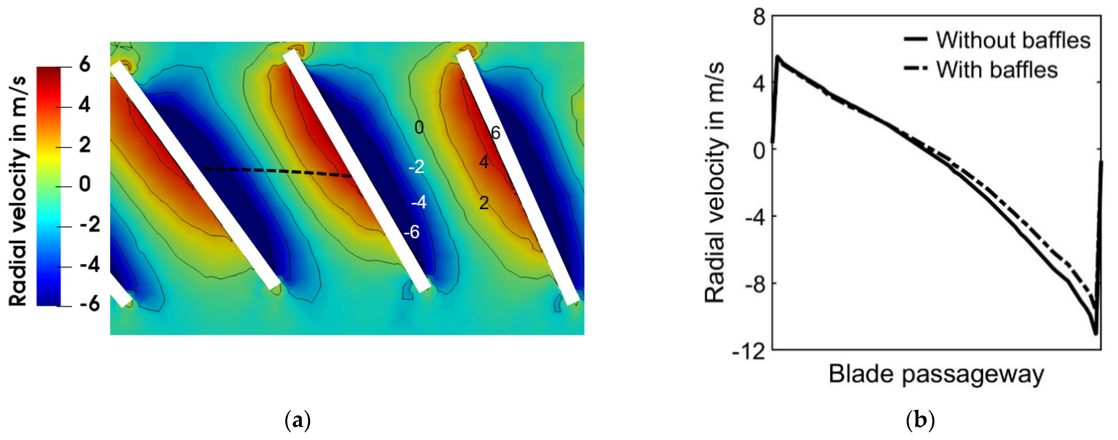
where $\eta$ is the dynamic viscosity of the air, $v_r$ is the radial velocity, $r$ is the radius, ${\rho }_P$ is the density of the solid particle and $v_{\phi }$ is the tangential velocity. Therefore, the cut size primarily depends on the radial and tangential velocities in the classifier. Classification takes place between the classifier blades. Figure 7 shows the radial velocity profile between two classifier blades. The classifier rotates clockwise, negative velocities point inward and positive velocities point outward. A vortex forms behind the leading blade, which constricts the radial transport inwards and significantly increases the radial velocity in zones where particles reach the inside. This effect increases with increasing classifier speed. Therefore, higher classifier speeds increase not only the tangential velocity, but also the radial velocity. However, since the tangential velocity has a quadratic influence on the cut-size, this influence is in general greater. Many studies have already investigated the flow profile and the influence of several parameters such as classifier speed or flow rate [7,9]. Therefore, this work focused exclusively on the effects of the flow baffles. Figure 4 shows that the installation of flow baffles reduced the tangential velocity inside the classifier, which also slightly reduced the tangential velocity between two classifier blades and deteriorated the classification efficiency of the classifier. With increasing speed, however, this effect decreased, since the relative proportion of the reduction of the tangential velocity became smaller and smaller. The right-hand side of Figure 7 shows that the baffles had a positive effect on the inward constriction of the radial transport.

Therefore, the radial velocity between two classifier blades (see left-hand side of Figure 7) for both classifier types is plotted. This effect improves the classification efficiency of the classifier and becomes more important at higher classifier speed. Both effects are superimposed and explain why the classifier without baffles separates better at lower speeds and the classifier with flow baffles has advantages in classification at high speeds.

4. Discussion

In this paper, the air flow inside a classifier was numerically investigated by applying Computational Fluid Dynamics (CFD). The DPM was employed to predict the motion of particles. Two different geometries at two operating conditions were compared to evaluate the effect of flow baffles within the classifier on flow profile, pressure loss and classification efficiency. For validation, a comparison with experimental data was carried out. The experimental results confirm those from the simulation. The results allow the following conclusions to be drawn.

Firstly, flow baffles inside the classifier break the vortex formation associated with an abrupt drop in tangential velocities inside the classifier. Therefore, a significant reduction in pressure drop is achieved. The reductions of the pressure loss depends on the operating conditions and reaches about 25% at high classifier speeds. Secondly, flow baffles also influence the grade efficiency of the classifier, as they have an impact on the radial and tangential velocities between the classifier blades. Therefore, the evaluation of the release properties is a function of the operating conditions. At low classifier speeds, the classifier without flow baffles separates better; at higher classifier speeds, the classifier with flow baffles separates better. Finally, the use of flow baffles depends on the operating conditions but is particularly suitable for high classifier speeds, which are usually associated with high energy costs. Thereby, the CFD is a suitable tool because it is a cost-effective and time-saving tool and provides a sufficiently accurate representation of characteristic values. With the help of numerical simulation, further investigations into the number and design of the flow baffles should be carried out in order to improve the flow processes in the classifier and operating costs.

References

1. Shapiro, M.; Galperin, V. Air classification of solid particles: A review. Chem. Eng. Process 2005, 44, 279–285. [Google Scholar] [CrossRef]
2. Batalović, V. Centrifugal separator, the new technical solution, application in mineral processing. Int. J. Miner. Process 2011, 100, 86–95. [Google Scholar] [CrossRef]
3. Johansen, S.T.; de Silva, S.R. Some considerations regarding optimum flow fields for centrifugal air classification. Int. J. Miner. Process 1996, 44–45, 703–721. [Google Scholar] [CrossRef]
4. Wang, X.; Ge, X.; Zhao, X.; Wang, Z. A model for performance of the centrifugal countercurrent air classifier. Powder Technol. 1998, 98, 171–176. [Google Scholar] [CrossRef]
5. Galk, J.; Peukert, W.; Krahnen, J. Industrial classification in a new impeller wheel classifier. Powder Technol. 1999, 105, 186–189. [Google Scholar] [CrossRef]
6. Bauder, A.; Müller, F.; Polke, R. Investigations concerning the seperation mechanism in deflector wheel classifiers. Int. J. Miner. Process. 2004, 74, 147–154. [Google Scholar] [CrossRef]
7. Toneva, P.; Epple, P.; Breuer, M.; Peukert, W.; Wirth, K.E. Grinding in an air classifier mill—Part I: Characterisation of the one-phase flow. Powder Technol. 2011, 211, 19–27. [Google Scholar] [CrossRef]
8. Stender, M.; Legenhausen, K.; Weber, A.P. Visualisierung der Partikelbewegung in einem Abweiseradsichter. Chem. Ing. Tech. 2015, 87, 1392–1401. [Google Scholar] [CrossRef]
9. Adamčík, M. Limit Modes of Particulate Materials Classifiers. Final Thesis, Brno University of Technology, Brno, Czech Republic, 2017. [Google Scholar]
10. Ren, W.; Liu, J.; Yu, Y. Design of a rotor cage with non-radial arc blades for turbo air classifiers. Powder Technol. 2016, 292, 46–53. [Google Scholar] [CrossRef]
11. Liu, R.; Liu, J.; Yuan, Y. Effects of axial inclined guide vanes on a turbo air classifier. Powder Technol. 2015, 280, 1–9. [Google Scholar] [CrossRef]
12. Yu, Y.; Ren, W.; Liu, J. A new volute design method for the turbo air classifier. Powder Technol. 2019, 348, 65–69. [Google Scholar] [CrossRef]
13. Sun, Z.; Sun, G.; Yang, X.; Yan, S. Effect of vertical vortex direction on flow field and performance of horizontal turbo air classifier. Chem. Ind. Eng. Prog. 2017, 36, 2045–2050. [Google Scholar] [CrossRef]
14. Sun, Z.; Sun, G.; Xu, J. Effect of deflector on classification performance of horizontal turbo classifier. China Powder Sci. Technol. 2016, 22, 6–10. [Google Scholar]
15. Kaczynski, J.; Kraft, M. Numerical Investigation of a particle seperation in a centrifugal air separator. Trans. Inst. Fluid-Flow Mach. 2017, 135, 57–71. [Google Scholar]
16. Guizani, R.; Mokni, I.; Mhiri, H.; Bournot, P. CFD modeling and analysis of the fish-hook effect on the rotor separator’s efficiency. Powder Technol. 2014, 264, 149–157. [Google Scholar] [CrossRef]
17. Barimani, M.; Green, S.; Rogak, S. Particulate concentration distribution in centrifugal air classifiers. Miner Eng. 2018, 126, 44–51. [Google Scholar] [CrossRef]
18. Guizani, R.; Mhiri, H.; Bournot, P. Effects of the geometry of fine powder outlet on pressure drop and separation performances for dynamic separators. Powder Technol. 2017, 314, 599–607. [Google Scholar] [CrossRef]
19. Osbaeck, B.; Johansen, V. Particle size distribution and rate of strength development of Portland cement. J. Am. Ceram. Soc. 1989, 72, 197–201. [Google Scholar] [CrossRef]
Figure 1. (a) Schematic view of experimental set-up; (b) geometry classifier and mill.
Processes 09 01213 g001
Figure 2. (a) Axial slice of mesh through static blades and classifier; (b) mesh of classifier.
Processes 09 01213 g002
Figure 3. Contour plots for the time averaged velocity in m/s for (a) mill and classifier without blades; (b) mill and classifier with twelve baffles at second operation conditions in Table 2.
Processes 09 01213 g003
Figure 4. Contour plots for the time averaged flow variables for the two types of air classifier at second operation conditions in Table 2. From top to bottom: the tangential velocity, the axial velocity, the radial velocity and the static pressure; (a) classifier without baffles; (b) classifier with baffles.
Processes 09 01213 g004
Figure 5. Particle trajectories for second operating condition in Table 2 and classifier with twelve baffles: blue 10 µm and red 50 µm.
Processes 09 01213 g005
Figure 6. Classification efficiency curves of the two types of classifier at two operating conditions in the simulation.
Processes 09 01213 g006
Figure 7. (a) Radial velocity profile between classifier blades without baffles; (b) comparison of radial velocity for classifier without and with baffles between classifier blades at second operation conditions in Table 2.
Processes 09 01213 g007