Article

Non-Intrusive Load Monitoring Based on Deep Pairwise-Supervised Hashing to Detect Unidentified Appliances

1
School of Control Engineering, Northeastern University at Qinhuangdao, Qinhuangdao 066004, China
2
School of Computer and Communication Engineering, Northeastern University at Qinhuangdao, Qinhuangdao 066004, China
*
Authors to whom correspondence should be addressed.
Processes 2021, 9(3), 505; https://doi.org/10.3390/pr9030505
Submission received: 14 December 2020 / Revised: 16 February 2021 / Accepted: 23 February 2021 / Published: 11 March 2021

Abstract

:
Non-intrusive load monitoring (NILM) is a fast developing technique for appliances operation recognition in power system monitoring. At present, most NILM algorithms rely on the assumption that all fluctuations in the data stream are triggered by identified appliances. Therefore, NILM of identifying unidentified appliances is still an open challenge. To pursue a scalable solution to energy monitoring for contemporary unidentified appliances, we propose a voltage-current (V-I) trajectory enabled deep pairwise-supervised hashing (DPSH) method for NILM. DPSH performs simultaneous feature learning and hash-code learning with deep neural networks, which shows higher identification accuracy than a benchmark method. DPSH can generate different hash codes to distinguish identified appliances. For unidentified appliances, it generates completely new codes that are different from codes of multiple identified appliances to distinguish them. Experiments on public datasets show that our method can get better F 1 - s c o r e than the benchmark method to achieve state-of-the-art performance in the identification of unidentified appliances, and this method maintains high sustainability to identify other unidentified appliances through retraining. DPSH can be resilient against appliance changes in the house.

1. Introduction

Information and Communication Technologies (ICT) and Intelligent Data Analytical Technologies (IDAT) have become the new trend for various industries’ development [1,2,3]. Following this trend, ICT and IDAT are increasingly implemented in multiple industries [4,5,6]. Load Monitoring is one of the ICT and IDAT implementation cases in the power system, and it can disaggregate the whole electricity consumption signal into the signals of appliances in a residential, commercial, or industrial building. Load monitoring can identify appliances and report consumers consumption patterns to improve consumer behavior [7]. Furthermore, finding the detailed electricity consumption patterns of the customers helps energy suppliers to efficiently plan and operate power system networks.
Traditional load monitoring equipment is intrusive, that is, a sensor with communication function is installed for one monitoring equipment in the total load, and then, the power consumption information is received through the network for real-time monitoring. This method requires a large number of sensors, which increases installation and maintenance costs. Unlike it, non-intrusive load monitoring (NILM) installs a smart meter at the user’s entrance to obtain the total current and terminal voltage. NILM can apply digital signal chemistry to the collected data, and then use algorithms to analyze and extract the power consumption information of various types of indoor appliances. The advantages of this method are as follows: low installation cost, little interference to users, and flexible application. Therefore, non-intrusive load monitoring technology has received widespread attention from scholars in recent years.
NILM was first proposed by Hart for residential load decomposition [8]. The operating states of appliances are divided into steady and transient. Therefore, the load monitoring methods can perform load decomposition based on steady or transient characteristics. The transient characteristics mainly include the change of the current or voltage waveform at the moment when the appliance starts. The duration of transient characteristics is short and unique, which can improve the recognition between loads. However, the transient feature extraction needs complex hardware, and the transient process of the load is affected by conditions such as grid voltage fluctuations, and the aging of electrical equipment. Steady-state load characteristics such as current harmonics [9], power harmonics [10,11], and current waveforms [12,13,
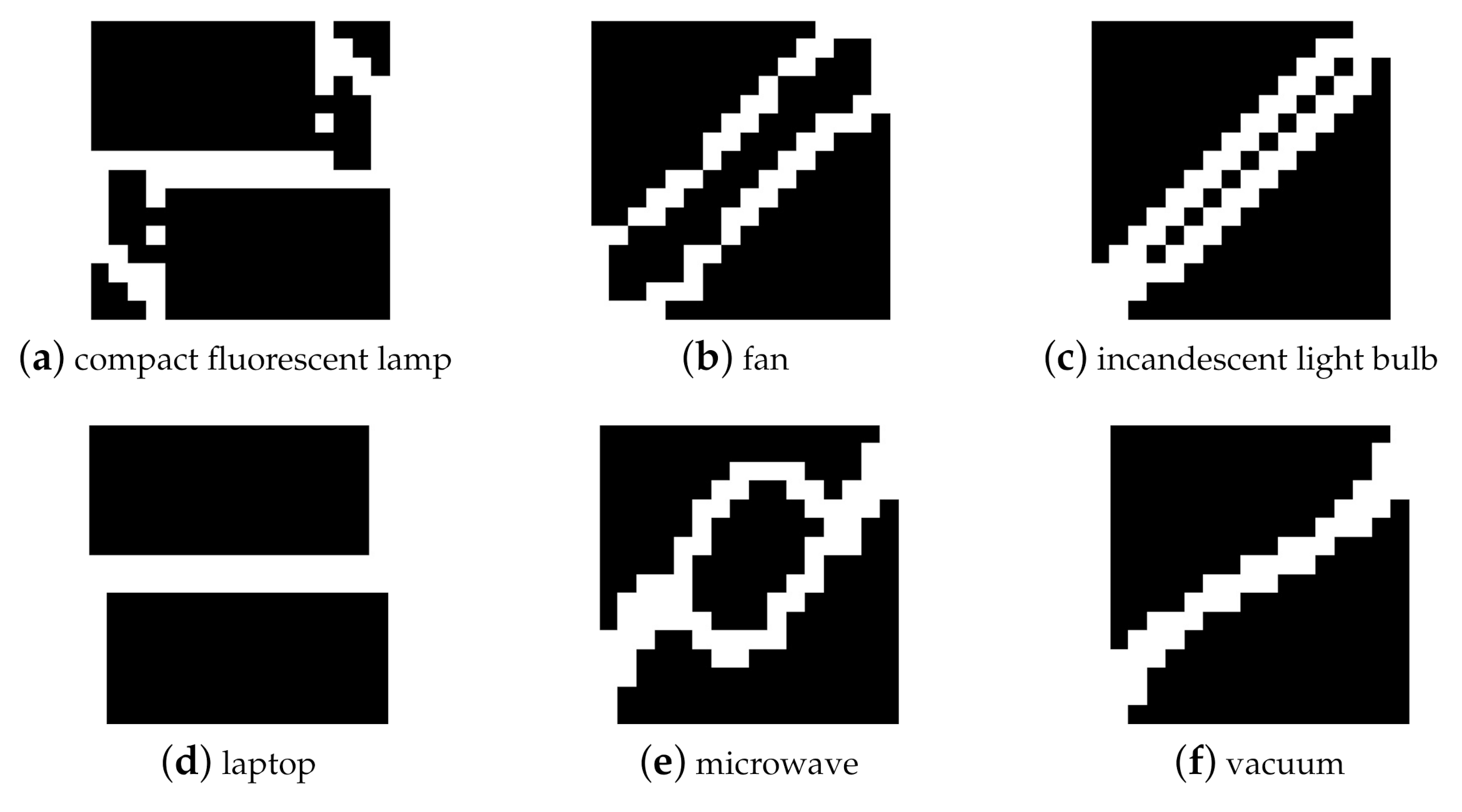
14] have been successively applied to NILM. Steady-state characteristics are generally obtained by index quantification. They are less affected by noise, but the probability of similarity of the single steady-state characteristics of the load increases when the number of loads rises. In order to distinguish multiple appliances, a new load characteristic that is V-I trajectory has been developed for NILM in recent years. The V-I trajectory is plotted based on the steady-state voltage and current, and it is used to express appliances’ electrical characteristics. The V-I trajectory in conjunction with many popular classification algorithms can offer better or generally comparable overall precision of prediction, robustness, and reliability [15]. In short, the V-I trajectory has advantages as a currently popular feature.
Based on different load characteristics, a variety of load identification algorithms have been proposed in NILM [16,17]. With the development of machine learning, the system results from the learning process can deliver the optimal predictive performance for appliance loads. Therefore, machine learning techniques have become a popular choice for NILM, since they showed significant disaggregation performance; in particular, Factorial Hidden Markov models (FHMMs) [18,19,20], Neural Networks (NN) [21,22,23,24], graph-based signal processing [25], Support Vector Machines (SVM) [26], k-Nearest Neighbours [26], and Decision Trees [27] have been successfully employed for NILM. Specifically, Reference [28] proposed a NILM algorithm based on features of the V-I trajectory. Ten V-I trajectory features were quantified based on physical significance, which accurately represented those appliances that had multiple built-in modes with distinct power consumption profiles, and the support vector machine multi-classification algorithm was employed for load identification. Reference [29] proposed a NILM algorithm based on the joint use of active and reactive power in the Additive Factorial Hidden Markov Models framework. In particular, in the proposed approach, the appliance model was represented by a bivariate Hidden Markov Model whose emitted symbols are the joint active-reactive power signals. The disaggregation was performed by means of an alternative formulation of the Additive Factorial Approximate Maximum a Posteriori (AFAMAP) algorithm for dealing with the bivariate HMM models. Reference [30] proposed an experimental design process for the application of energy disaggregation using multi-label classification. This paper took the electrical parameters of the current (I), real power (P), reactive power (Q), and power factor (PF) at every one-minute and employed RAndom k-labELsets (RAkEL) with Decision Tree as the multi-label classification algorithm together with the right model parameter configuration.
However, it is worth noting that most classification algorithms described in the literature cannot identify unidentified appliances in the consumer environment. In these algorithms, the unidentified appliance will be assigned a label and power consumption. They correspond to the identified appliance which have the most similar features. This leads to confusion between the identification of identified appliances and unidentified appliances. At the same time, the accuracy of appliance identification is reduced. Therefore, the household power consumption that is fed back to consumers and the power department is inaccurate.
Considering that the V-I trajectory is an image feature, its application enables NILM to be transformed into image retrieval. With the explosive growth of data in real applications like image retrieval, approximate nearest neighbor (ANN) search [31] has become a hot research topic in recent years. Due to its fast query speed and low memory cost, hashing [32] has become one of the most popular and effective techniques among existing ANN techniques. Existing hashing methods can be divided into data-independent methods and data-dependent methods. In data-independent methods, the hash function is typically randomly generated. It is independent of any training data. The representative data-independent methods include locality-sensitive hashing (LSH) [33] and its variants. Data-dependent methods try to learn the hash function from some training data, and they are also called learning to hash (L2H) [34] methods. Compared with data-independent methods, L2H methods can achieve comparable or better accuracy with shorter hash codes. Representative learning to hash methods include fast supervised hashing (FastH) [35], supervised discrete hashing (SDH) [36], column-sampling based discrete supervised hashing (COSDISH) [37], and column generation hashing (CGHash) [38].
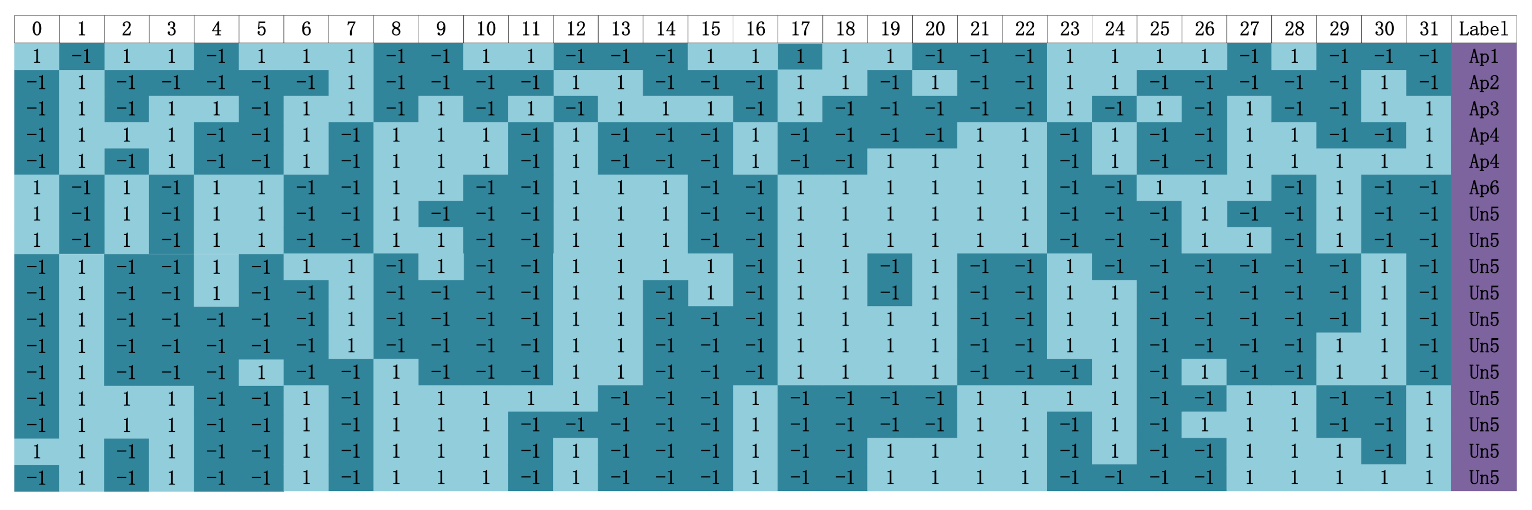
Therefore, this paper proposes a V-I trajectory enabled deep pairwise-supervised hashing (DPSH) method for NILM. It contains simultaneous feature learning and hash-code learning. DPSH encodes the V-I trajectory images of identified appliances into compact binary hash codes. According to different coding results, we can identify various identified appliances in the environment, and DPSH can detect previously unidentified appliances in an automated way. When there is an unidentified appliance, DPSH will encode the V-I trajectory images of this appliance into brand new hash codes, which are different from other identified appliances. Thence, our proposed method can provide a scalable solution to energy monitoring for contemporary unidentified appliances.
The main contributions of this paper can be summarized as follows:
Firstly, to the best of our knowledge, DPSH which can perform simultaneous feature learning and hash-code learning for applications with pairwise labels is first applied to NILM. This method transfers appliance identification to approximate nearest neighbor search, and improves the identification accuracy of identified appliances.
Secondly, the majority of the NILM approaches are sensitive to the replacement and addition of appliances in the house, and thus require regular retraining. In this paper, the focus lies on creating a classification algorithm that is able to detect unidentified appliances. Therefore, the algorithm can be resilient against the replacement and addition of appliances in the house. If an unidentified appliance is detected, labeling and retraining are requested to restore the identified environment and then identify the next unidentified appliance.
Thirdly, this paper also reflects the retraining results of our proposed method after identifying the unidentified appliance. The results show that the identification accuracy of DPSH can be restored to a high level through retraining, and when the next unidentified appliance appears, DPSH can still recognize it. In other words, DPSH maintains high sustainability. Experiments on public datasets show that DPSH can outperform the benchmark method to achieve state-of-the-art performance in NILM.
This paper is organized as follows. Section 2 defines some symbols and issues in DPSH method. Section 3 explains the model and learning process of DPSH method as well as how it can be used for load disaggregation. 
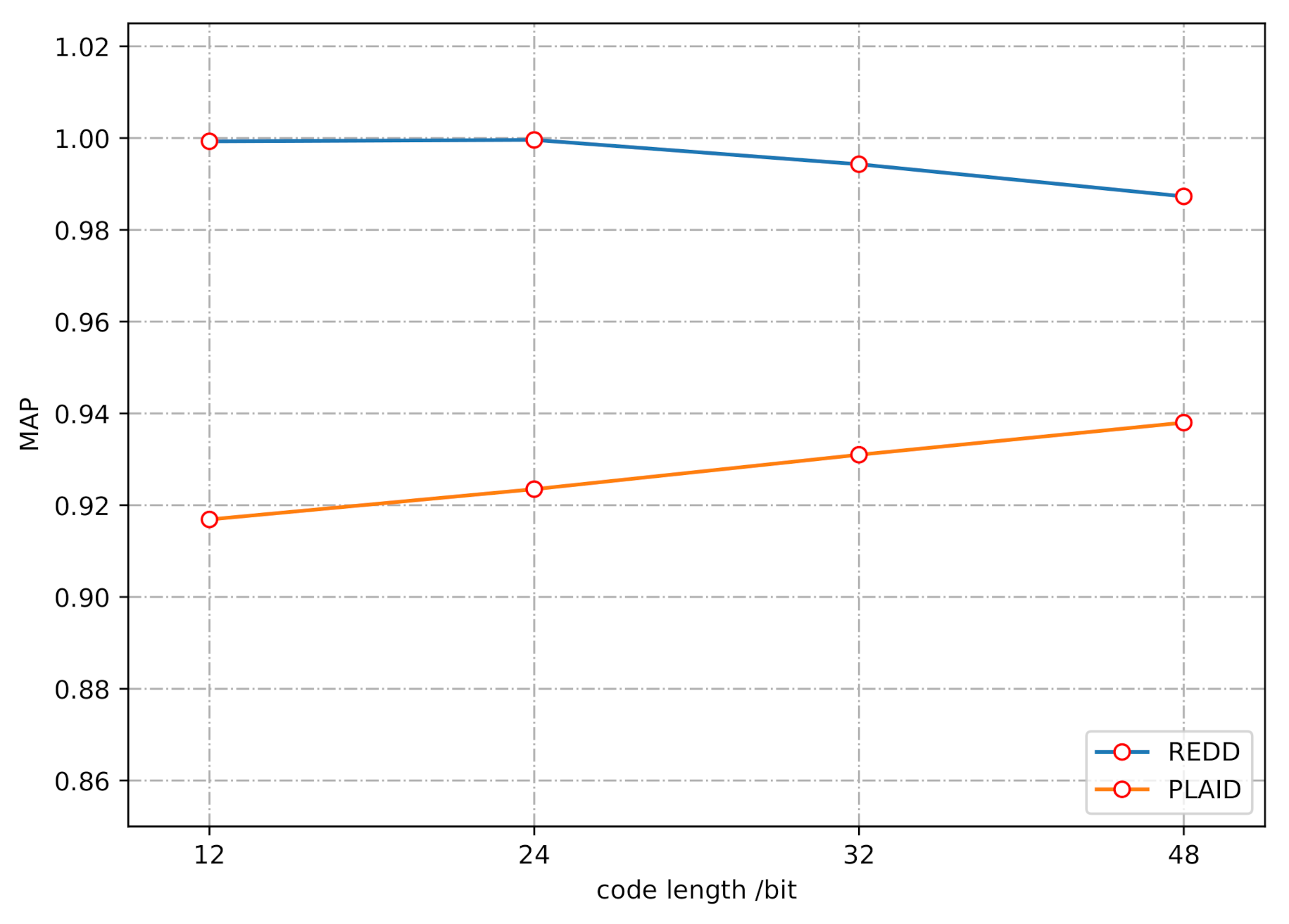
Section 4 introduces benchmark datasets, the input of network, performance metrics, and selection of code length. The experimental results on publicly available datasets are presented in Section 5 to evaluate the performance of the proposed DPSH method for NILM. Moreover, the conclusions are given in Section 6.

2. Notation and Problem Definition

We convert the classification of electrical appliances to approximate nearest neighbor search of V-I trajectories in this paper.

2.1. Notation

The lowercase letters like z are used to denote vectors. We use uppercase letters like Z to denote matrices. Z T denotes the transpose of Z. The Euclidean norm of a vector is denoted as | | · | | 2 . s g n ( · ) is used to denote the element-wise sign function. If the element is positive, s g n ( · ) will return 1. Otherwise it will return −1.

2.2. Problem Definition

Suppose we have n V-I trajectory images X = { x i } i = 1 n where x i is the i-th element in set X. Besides the set of V-I trajectories, the training set of supervised hashing with pairwise labels also contains a set of pairwise labels S = { s i j } n × n with s i j { 0 , 1 } . s i j = 1 denotes V-I trajectory x i is similar to V-I trajectory x j . Otherwise, they are dissimilar. Here, the pairwise labels typically refer to semantic labels provided with manual effort.
The goal of supervised hashing with pairwise labels is to classify V-I trajectories correctly by learning hash function h ( x ) . We can get a binary code b i { 1 , 1 } c for every trajectory x i , where b i = h ( x i ) = [ h 1 ( x i ) , h 2 ( x i ) , . . . , h c ( x i ) ] , and c means the length of code. All of binary codes are collected in the set B = { b i } i = 1 n . The similarity in S should be preserved in the binary codes B. If s i j = 1 , it means that the Hamming distance between the binary codes b i and b j should be as small as possible. Otherwise s i j = 0 , when the binary codes b i and b j have a high Hamming distance.

3. Deep Pairwise-Supervised Hashing

In this section, we introduce the DPSH model based on the V-I trajectory in detail. This section contains the model composition and learning algorithm.

3.1. Model Composition

The workflow of the proposed method that is able to detect unidentified appliances is shown in Figure 1. In the training phase, a hash function that can encode samples of the same appliance into the same binary hash codes is computed from the V-I trajectory images by training the feature learning part. The V-I trajectory images must be paired and labeled respectively as must- or cannot-links. This depends on if the images belong to the same class or not. The transformation does not depend on the appliance label. On the transformed input, DPSH determines the final encoding results of each identified appliance by minimizing pairwise loss. In the test phase, a V-I trajectory image is encoded to a kind of only binary hash codes. Next, we calculate the Hamming distance (d) to all representation codes. If the distance is equal to zero, the V-I trajectory is classified as one of the identified appliances. If the distance is not equal to zero, the trajectory is labeled as ‘’unidentified’’.
DPSH model has an end-to-end deep learning architecture, which contains two essential parts: feature learning part and objective function part, and it is shown in Figure 2. Specifically, the feature learning part and objective function part feedback with each other during the training procedure. Feature learning part aims to learn a deep neural network which can extract multiple features from V-I trajectory images, and then features are encoded into compact binary hash codes. The goal of objective function part is to learn how to encode the features, which can reflect the supervised information (similarity) between two V-I trajectory images. The combination of the two parts achieves the purpose of load identification.

3.1.1. Feature Learning Part

Convolutional neural network (CNN) is a type of neural networks (NNs) that are often used in computer vision because they are highly suitable to classify images. We adopt a classical CNN model to extract the features of V-I trajectory images in this part. The feature learning part contains the Alexnet [39] model as a component, which has eleven layers and is good at extracting the features of images. The structure of the DPSH model is symmetrical. In other words, there are two Alexnets (top Alexnet and bottom Alexnet) in the feature learning part. These two Alexnets have the same structure and share weights. That is to say, the input of the model are pairs of V-I trajectories and pairwise labels between the trajectories. The feature learning part is an indispensable foundation for NILM.
The network structure and parameters of the Alexnet model have been introduced in Table 1. More specifically, there are 5 convolutional layers (Conv 1–5), 3 max-pooling layers (MaxP 1–3), and 3 fully connected layers (FC 1–3) in the Alexnet model. The role of the convolutional layers is to extract local features of the trajectories. The progress of Alexnet is to imitate a large receptive field effect by using multiple convolution kernels in sequence. Alexnet uses convolution kernels and pooling kernels to deepen the network structure continuously and improve performance. The max-pooling layers are used to reduce the size of images, and fully connected layers are to reassemble the extracted local features into a complete graph through the weight matrix. The parameters of the Alexnet model are mainly concentrated in three fully connected layers. As shown in Table 1, the size of the convolution kernels in each segment gradually decreases, and the pooling kernels’ size in each segment is the same.

3.1.2. Objective Function Part

We can define the likelihood of pairwise labels S = { s i j } n × n as follows, when the binary codes B = { b i } i = 1 n for all the V-I trajectory images are given.
p ( s i j | B ) = σ ( Ω i j ) , s i j = 1 1 σ ( Ω i j ) , s i j = 0
where Ω i j = 1 2 b i T b j , and σ ( Ω i j ) = 1 1 + e Ω i j . Ω i j means half of the inner product of two codes. When the two codes are the same, the inner product is the largest. In contrast, when two codes are completely different, the inner product is the smallest, so Ω i j can indicate the similarity of two codes. It is worth noting that b i { 1 , 1 } c .
By taking the negative log-likelihood of the pairwise labels observed in S, we can get the following optimization problem:
min B J 1 = log p ( S | B ) = s i j S log p ( s i j | B ) = s i j S ( s i j Ω i j log ( 1 + e Ω i j )
The optimization problem in (2) fully reflects the goal of supervised hashing with pairwise labels. The Formula (2) ensures that the Hamming distance between two similar V-I trajectory images can be as small as possible, while the Hamming distance between two dissimilar V-I trajectory images can be as large as possible. Therefore, the purpose of distinguishing various appliances through the V-I trajectories is achieved.
However, the problem in (2) is a discrete optimization problem that is hard to solve. Although it is solved by (1), directly relaxing B = { b i } i = 1 n from discrete to continuous, satisfactory performance still cannot be obtained. Therefore, we adopt a novel strategy that can directly solve the problem in (2) in a discrete way. In other words, there is no need to give up the accuracy of B and convert it. We reformulate the problem in (2) as the following equivalent problem:
min B , U J 2 = s i j S ( s i j Θ i j log ( 1 + e Θ i j ) s . t . u i = b i , i { 1 , 2 , . . . , n } u i R c × 1 , i { 1 , 2 , . . . , n } b i { 1 , 1 } c , i { 1 , 2 , . . . , n }
where Θ i j = 1 2 u i T u j , and U = { u i } i = 1 n .
To optimize the above problem, we can move the equality constraints in (3) to the regularization terms, so we reformulate the optimize problem (3) as the following equivalent one:
min B , U J 3 = s i j S ( s i j Θ i j log ( 1 + e Θ i j ) + η i = 1 n b i u i 2 2
where η is the regularization term that is a hyper-parameter.

3.1.3. DPSH Model

The DPSH model uses an end-to-end framework, which integrates the above feature learning part and objective function part together, and the end-to-end framework is expressed as
u i = W T ϕ ( x i ; θ ) + v
where the network parameters of Alexnet model in the feature learning part are denoted as θ . Furthermore, We define the output of the Alexnet model with the network parameter θ as ϕ ( x i ; θ ) , when the V-I trajectory image x i is used as the input of the Alexnet model. W R 1000 × c is a weight matrix, and v R c × 1 denotes a bias vector. That is to say, our DPSH model integrates the feature learning part and the objective function part into an end-to-end framework through a weight matrix and a bias vector. This method is similar to the function of a fully connected layer. After integrating the two parts, the final problem becomes
min B , W , v , θ J = s i j S ( s i j Θ i j log ( 1 + e Θ i j ) + η i = 1 n b i ( W T ϕ ( x i ; θ ) + v ) 2 2
Therefore, we get an end-to-end DPSH model. It can perform both feature learning and hash-code learning simultaneously in the same framework. The method can generate different hash codes to distinguish identified appliances and a completely new kind of hash codes for the unidentified appliance.
In conclusion, DPSH contains three key components. The first component is a deep neural network to learn image features from pixels. The second component is a hash function to map the learned image features to hash codes, and the third component is a loss function to measure the quality of hash codes guided by pairwise labels.

3.2. Learning Algorithm

In the DPSH model, known parameters include the pairwise labels S and the regularization term η . Other parameters including W, v, θ , and B need to be learned. In this paper, we adopt a minibatch-based strategy for learning. That is to say, in each iteration, we sample a mini-batch of V-I trajectory images from the whole training set, and then we can perform learning based on these sampled V-I trajectory images, and we design a method of alternating learning. More specifically, we optimize one parameter while other parameters are fixed. The hash codes b i can be directly optimized as follows:
b i = s g n ( u i ) = s g n ( W T ϕ ( x i ; θ ) + v )
where s g n ( · ) can extract the sign of the input.
We adopt the back-propagation (BP) algorithm to calculate the gradient in order to update other parameters W, v, and θ . In particular, we can calculate the derivative of the loss function with regard to u i according to the following formula:
J u i = 1 2 j : s i j S ( a i j s i j ) u j + 1 2 j : s i j S ( a j i s j i ) u j + 2 η ( u i b i )
where a i j = σ ( 1 2 u i T u j ) .
Then, we can calculate the gradient and use back-propagation algorithm to update the parameters W, v, and θ respectively:
J W = ϕ ( x i ; θ ) ( J u i ) T
J v = J u i
J ϕ ( x i ; θ ) = W J u i

4. Experiment

4.1. Tool and Environment

All the experiments are implemented using Python 3.6 on a standard PC with an Intel Core i7-6700MQ CPU running at 3.40 GHz and with 16.0 GB of RAM. The CNN architecture is constructed based on Pytorch, and the pre-trained CNN model is migrated to DPSH.

4.2. Benchmark Datasets

The performance of the proposed algorithm is validated on the Reference Energy Disaggregation Data Set (REDD) and the Plug-Level Appliance Identification Dataset (PLAID).

4.2.1. REDD Dataset

REDD is a freely available data set containing detailed power usage information from several homes. It is aimed at furthering research on energy disaggregation [40]. The data contains power consumption from real homes over several months’ time. They are the power consumption of the whole house as well as for each individual circuit in the house. All data in REDD is recorded with UTC time stamps. For each monitored house, REDD record the AC waveform itself in order to compute both real and reactive powers easily. This dataset includes low-frequency power data in each house, high-frequency voltage, and current data in house 3 and house 5. The list of appliances in the REDD dataset has been introduced in Table 2.

4.2.2. PLAID Dataset

The Plug-Level Appliance Identification Dataset is a public and crowd-sourced dataset for load identification research. PLAID dataset includes short voltage and current measurements for different residential appliances. The measurement equipment collects data in the order of a few seconds. The goal of PLAID is to provide a public library for high-resolution appliance measurements. It can be integrated into existing or novel appliance identification algorithms [41]. PLAID currently includes current and voltage measurements sampled at 30 kHz from 11 different appliance types present in more than 60 households in Pittsburgh, Pennsylvania, USA. Data collection took place during the summer of 2013 and winter of 2014. Measurements with significant noise in the voltage due to measurement errors were removed [42]. The list of appliances in the PLAID dataset has been introduced in Table 3.

4.3. The Input and Architecture of DPSH

Our paper adopts an event detection method and a trajectory extraction method, which are proposed in Reference [28]. An event is defined as the state-switching process of an appliance within a certain period of time. In this paper, the event is detected by comparing the variation in power during that durations with two predetermined thresholds.
| Δ P t | P o n 1 & | Δ P t + 1 | P o n 1 & . . . & | Δ P t + T R 1 | P o n 1 & | Δ P t + T R | < P o n 1 & | Δ P t + T R + 1 | < P o n 1 & | P t + T R P t | P o n 2
Event detection is summarized by (12). Stride is represented by R in (12), and R is set to 1 s. The aggregated apparent power at t s is P t . The difference between two adjacent aggregated apparent powers is denoted by Δ P t ( Δ P t = P t + 1 P t ). The event begins when | Δ P t | P o n 1 , and continues to calculate | Δ P t + 1 | , | Δ P t + 2 | , . . . , until | Δ P t + T R | < P o n 1 and | Δ P t + T R + 1 | < P o n 1 . If | P t + T R P t | P o n 2 , the appliance has a state transition at t t + T R s. In other words, the integral event begins at t s and finishes at t + T R s. T is the number of strides that represents the duration of the event. P o n 1 and P o n 2 are set as 30W and 100W respectively in this paper. We believe that power fluctuations below P o n 1 are considered to be caused by noise, and it is considered a complete state switching process that the power difference before and after the event is greater than P o n 2 , and event detection is an essential step for V-I trajectory extraction. The voltage and current data must be processed before plotting the trajectory.
We extract the same number of voltage and current waveforms before and after the event. Four kinds of waveforms (the voltage waveforms before the event, the current waveforms before the event, the voltage waveforms after the event, and the current waveforms after the event) are interpolated and averaged separately. Then, the voltage waveforms before and after the event are averaged. The current waveform before and after the event takes the difference. Therefore, we can plot the V-I trajectory as a delta-form signature, which makes use of the difference between two consecutive snapshots and meets the feature-additive criterion [12]. We extracted 10 types of appliances’ V-I trajectories from the REDD dataset to verify the effectiveness of our proposed method. According to the above method, the V-I trajectories for different appliances from REDD database are shown in Figure 3. Then, we directly use the raw images as input in DPSH model. We extract 4400 V-I trajectory images to train the proposed model. Each image belongs to one of the 10 classes. For these classes, the number of images of each class is at least 100, and we randomly select 1100 V-I trajectory images for the test set.
PLAID is a data set composed directly of the voltage and the current data of many appliances. It requires the same data processing to extract the trajectory. However, PLAID dataset is different from REDD dataset. PLAID currently includes current and voltage measurements sampled from different appliance types present in more than 60 households. We need a method to reduce the fluctuation of the image shape, so we convert every V-I trajectory image into a binary V-I image ( n × n matrix) by meshing the V-I trajectory. Each cell of the mesh is assigned a binary value that denotes whether or not it is traversed by the trajectory. Binary V-I image can reduce the volatility of data generated by different appliance types present in different households, and we choose 6 binary V-I trajectory images to test DPSH algorithm, as shown in Figure 4. We select 757 V-I trajectory images to train the proposed model. Each image belongs to one of the 6 classes. For these classes, the number of images of each class is different. The category with the fewest numbers contains 26 images, and we randomly select 226 V-I trajectory images for the test set.
All of the V-I trajectory images are resized as 224 × 224. Then we directly use the raw image pixels as input in DPSH model. Please note that there are two Alexnets (top Alexnet and bottom Alexnet). These two Alexnets have the same structure and share the same weights. That is to say, both the input and the loss function are based on pairs of images. The extracted V-I trajectories are input into the Alexnets in pairs. The features of V-I trajectories, which are extracted after 5 convolutional layers, 3 max-pooling layers, and 3 fully connected layers, form many feature vectors of 1000 elements. DPSH model learns a hashing function can convert 1000-dimensional feature vectors to trajectory codes in the training period. The code length is a hyper-parameter. We can set it according to our own needs. The trajectory codes must ensure that the Hamming distance between two similar V-I trajectory images is as small as possible, while the Hamming distance between two dissimilar V-I trajectory images is as large as possible. In other words, the trajectory codes can reflect pairwise similarity. Therefore, we can identify the category information of V-I trajectories according to these codes in the testing period. Two V-I trajectories will belong to the same category if the Hamming distance between two trajectory codes is close to 0, and the proposed model can produce a lot of coding results that have never been seen in the training period when there are unidentified appliances in the consumer’s environment. At this point, we can retrain the model quickly to accommodate the addition of a new appliance. The retrained model can also continue to detect other newer appliances.

4.4. Performance Metrics

In this paper, the problem of NILM is considered as an approximate nearest neighbor search task, which should assign each V-I trajectory image into one of predefined classes. We utilize a meaningful performance metric, mean average precision ( M A P ), which can illustrate the performance in many multi-class classification tasks [43]. We estimate the ranks of data samples in the calculation of average precision( A P ). The discrete form of A P for class C k is
A P k = 1 | C k | x i C k r a n k ( s i ; { s j | x j C k } ) r a n k ( s i ; { s j | x j X } )
where we use x i to represent the ith query V-I image. | C k | denotes the cardinality of set C k , and r a n k ( s ; S ) is the rank of s in set S. A smoothed pair-wise rank function can be used to estimate ranking relation between two samples x i and x j . This function is defined in [42] as follows.
r a n k ( x i ; x j ) = 1 1 + e α k [ d k ( x i ) d k ( x j ) ]
For M-class classification, we will generally use the mean of all A P s of different classes to evaluate the overall performance.
M A P = 1 M k = 1 M A P k
We adopt three classification metrics to evaluate the effect of classification. They are shown in the following equations based on True Positive ( T P ), True Negative ( T N ), False Positive ( F P ), and False Negative ( F N ). These metrics analyze how well the algorithm can identify changes in the appliance’s status.
P r e c i s i o n = T P T P + F P
R e c a l l = T P T P + F N
F 1 - s c o r e = 2 × P r e c i s i o n × R e c a l l P r e c i s i o n + R e c a l l
F 1 - s c o r e is a measure of the test’s accuracy and is obtained by calculating the weighted average of the P r e c i s i o n and R e c a l l . It calculates the percentage of energy correctly assigned to each appliance in the dataset. A higher F 1 - s c o r e value indicates a better identification of the appliance. To obtain the final test result, the average F 1 - s c o r e is taken:
F a v e r a g e = i = 1 N F 1 , i
where N is the amount of different appliances, and F 1 , i is the F 1 - s c o r e when appliance i is used as hold out appliance.

4.5. Selection of Code Length

We adopt the REDD dataset and PLAID dataset to verify the performance of DPSH. In the experiment on each dataset, both training and testing are done on all of the appliances. The number of V-I trajectory images produced by each kind of appliance has a different proportion in the total. The reason is that the frequency of opening and closing is different in the operation of various appliances. We adopt a pre-trained Alexnet model to reduce training times. Besides, we set the mini-batch size to be 64 and tune the learning rate among [ 10 6 , 10 2 ] . For DPSH method, the hyper-parameter η is set to be 50 by using a validation strategy. The most important parameter is the length of the output hash code. The optimal code length determines the recognition accuracy and space complexity of DPSH algorithm. Therefore, the code length is set to be 12, 24, 32, 48 bits [35,36,37] so that we can verify the effect of this parameter on experimental results. As shown in Figure 5, the DPSH method based on the Alexnet model shows high accuracy in terms of M A P when the code length is set to be 12, 24, 32, 48 bits.
Figure 5 shows that the M A P of DPSH for different code lengths. The specific values of M A P are 0.9993, 0.9996, 0.9943, and 0.9873 when DPSH is tested on the REDD dataset. Meanwhile, the performances of our proposed method on the PLAID dataset are 0.9169, 0.9235, 0.9310, and 0.9380 in the form of M A P . It can be seen that the performance of DPSH on REDD is better than that on PLAID. This is because we believe that there is only one V-I trajectory for each appliance when processing the REDD dataset, and the V-I trajectory shape of each appliance is different in the PLAID dataset. In other words, we assume that all 10 appliances in the REDD dataset are single-state appliances (Each appliance corresponds to a V-I trajectory). In the PLAID dataset, there are many types of V-I trajectories for each appliance. This may be a normal multi-state appliance, or it may be caused by measurement errors, and the part of trajectories of various appliances may be repeated. This is the reason why the results on REDD and PLAID are different. However, DPSH can maintain high accuracy in both two datasets, as shown in Figure 5. The minimum value of M A P in the PLAID dataset reaches 0.9169, when the code length is set to be 12 bits.
According to the above analysis, the M A P of DPSH on the two datasets is high and the performance is stable. Through calculation, we get the average M A P of each code length as 0.9581, 0.9616, 0.9627, and 0.9627. It can be seen that the M A P value of 0.9627 is the best result, but the average M A P of 32 bit and 48 bit are equivalent. At the same time, a too-long code length will increase memory cost, so we chose 32 bit as the code length for subsequent result analysis.

5. Results and Discussion

To define how well the DPSH model can identify identified appliances and unidentified appliances, we designed the following two scenarios. Scenario 1 simulates a normal household electricity environment where all of appliances are identified. Scenario 2 simulates a household environment where unidentified appliance exists.

5.1. Recognition of Identified Appliances

We train and test on two datasets to verify whether the proposed algorithm can distinguish identified appliances well. The number of appliances used for training and testing is the same, and Table 4 details the performance indicators achieved by running DPSH with 32-bit code length on different datasets. These are the best results of our proposed method on two datasets. As shown in Table 4, the P r e c i s i o n , R e c a l l , and F 1 - s c o r e of every appliance are introduced in detail. This shows that our proposed algorithm is highly effective in appliance identification. It can accurately identify all appliances in REDD. DPSH also has a good ability to identify all appliances in the PLAID dataset. In conclusion, this method has a strong adaptability to different datasets.
The 32-bit encoding results of DPSH method on the PLAID dataset are shown as Figure 6. It ensures that the Hamming distance between codes of different labels is as large as possible, but a kind of appliance label does not necessarily correspond to only one encoding result. This phenomenon illustrates the complexity of the PLAID dataset, and multiple encoding results of DPSH increase the stability of the method. It ensures that the algorithm can still maintain a high accuracy of appliance identification when the V-I trajectory images of the appliance are deviated due to fluctuations or the appliance has multiple states.
The benchmark method in Reference [44] is based on siamese neural network and DBSCAN clustering method (SN-DBSCAN). Figure 7 is the P r e c i s i o n and R e c a l l for proposed DPSH and SN-DBSCAN [44] algorithm on REDD and PLAID datasets. The appliances in Figure 7 correspond to Table 2 and Table 3. Figure 7a,b reflects the results generated by testing on REDD. It is obvious that the P r e c i s i o n and R e c a l l for DPSH-32-bit are stable. The P r e c i s i o n for the SN-DBSCAN algorithm has a slight deviation. However, the R e c a l l for the SN-DBSCAN algorithm has great fluctuation. It has the lowest R e c a l l value for the third appliance, only 0.556. Meanwhile, as shown in Figure 7c,d, the results on the PLAID dataset are similar to the above. The P r e c i s i o n and R e c a l l for DPSH-32-bit only fluctuate a little bit and are basically stable at very high values. Due to the complexity of PLAID, the P r e c i s i o n and R e c a l l for DPSH-32-bit have some fluctuations on the second and third appliances. The R e c a l l value of the second appliance is the lowest, but it has reached 0.882. The P r e c i s i o n and R e c a l l of SN-DBSCAN not only have lower values on the second and third appliances but also have larger deviations on other appliances. This shows that DPSH is more stable on a complex PLAID dataset than SN-DBSCAN. In other words, this demonstrates that DPSH leads to performance improvements with respect to the SN-DBSCAN even in the presence of noise or measurement error. After the above analysis, it specifically reflects that DPSH is always more accurate than the SN-DBSCAN algorithm. We can conclude from Figure 7 that our proposed algorithm maintains high P r e c i s i o n and R e c a l l on REDD and PLAID to ensure high accuracy of appliance identification.
The radar chart in Figure 8 shows the F 1 - s c o r e for each appliance in the experiment including two datasets, and the area of each colored line is proportional to the F a v e r a g e of the related algorithm. It shows that the DPSH method gives better results for every appliance on F 1 - s c o r e , compared with the SN-DBSCAN algorithm. The F a v e r a g e of DPSH and SN-DBSCAN are 0.984 and 0.932 on REDD, respectively, and the indicators on the PLAID dataset are 0.969 and 0.815. The more complex the test environment, the greater difference in F a v e r a g e between DPSH and SN-DBSCAN. Compared with the SN-DBSCAN algorithm, the experimental results indicate that the proposed method significantly improves the accuracy and can be efficiently generalized when they are tested on the same database.

5.2. Recognition of Unidentified Appliance

To define how well the method can identify unidentified appliances, we complete the experiment on two datasets. We choose the Ap10 to be an unidentified appliance and call it Un10 in the REDD dataset. All other appliances are identified appliances, so training is done on 9 appliances and testing on 10 appliances. Similarly, we choose the Ap5 to be an unidentified appliance and call it Un5 in the PLAID dataset, and training is done on 5 appliances and testing on 6 appliances. The goal of our experiments is to detect unidentified appliances in user environments. Therefore, we choose Un10 and Un5, respectively, in two datasets as fixed unidentified appliances. This is called leave-one-appliance-out validation. In the REDD, each appliance corresponds to one V-I trajectory, but there is more than one V-I trajectory for each of these appliances in the PLAID, and they may be similar to each other, so we designed two experiments on two different datasets. It is validated whether (1) the selected appliances are properly separated by different codes with high Hamming distance, and (2) the unidentified appliance has its trajectory images classified as “unidentified”.
The 32-bit encoding results of DPSH method on the PLAID are shown as Figure 9 when the last appliance is selected to be unidentified. Compared with Figure 6, we can see that the encoding results of the unidentified appliance are different from the encoding results of the identified appliances and include several forms. Therefore, our proposed method can achieve the purpose of detecting the unidentified appliance. Note that the encoding results of the same labels in Figure 6 and Figure 9 are different. Because the samples used to learn the hash function are different (in Figure 9, the samples for the fourth appliance are not used).
To know which appliances are mixed up, a confusion matrix is created: Figure 10a,b reports for each appliance type (row index) the number of labels that were correctly predicted or confused with other appliances (column index). The values in the matrix are percentages, and the colors represent the recall value per row (thus per appliance). It can be seen that the recognition accuracy of the appliances used for training is still very high. Due to measurement errors or similar shapes to other appliances, the unidentified appliance is encoded into a variety of discrete hash codes, so the unidentified appliance may be confused with other appliances. On the REDD dataset, only a small number of identified appliances are distinguished as unidentified. All the unidentified appliances are distinguished and marked correctly. Due to the complexity of the environment, the identified and unidentified appliances are confused on the PLAID, during the process of differentiation, but the number is small. In conclusion, we can discover that the DPSH algorithm also has high accuracy for the identification of unidentified appliances by analyzing the experimental results on the two datasets.
According to Reference [44], the training appliances are used for learning form clusters. The samples belonging to the holdout appliance do not belong to any cluster and neither form a cluster as the siamese neural network is not trained on them. They have spread around and get the label “unidentified”. We train and test SN-DBSCAN on the same datasets. The experimental results of the two methods on REDD and PLAID with the unidentified appliance are shown in Table 5 and Table 6. For all appliances, the recognition accuracy of DPSH is basically higher than that of SN-DBSCAN. At the same time, we find that DPSH can maintain a high recognition capability for identified appliances.
F 1 - s c o r e is an evaluation that comprehensively considers P r e c i s i o n and R e c a l l and can more fully reflect the appliance identification. Therefore, we next focus on this indicator. The radar chart in Figure 11 shows the F 1 - s c o r e for each appliance in the experiment, including all the appliances in two datasets. In the REDD experiment, the F 1 - s c o r e of DPSH on Ap1 and Ap2 are slightly lower than SN-DBSCAN. On Ap1 and Ap2, especially on the unidentified appliance, DPSH’s F 1 - s c o r e are significantly higher than SN-DBSCAN, and the F a v e r a g e values of DPSH and SN-DBSCAN are, respectively, 0.942 and 0.860. In the PLAID experiment, DPSH can better identify the unidentified appliance, but the F 1 - s c o r e of DPSH on Ap2 and Ap6 are slightly higher than SN-DBSCAN. The F a v e r a g e values of two algorithms are, respectively, 0.883 and 0.726. When unidentified appliances appear in the environment, although the SN-DBSCAN algorithm can identify them, the recognition accuracy of the identified and unidentified appliances decreases significantly. Concerning SN-DBSCAN algorithm, the proposed approach shows a higher improvement. The relative differences of F a v e r a g e are +0.082 and +0.157. In conclusion, the recognition ability of DPSH is very prominent for both identified appliances and the unidentified appliance.
To further illustrate the effectiveness and practicality of DPSH, this paper conducts retraining experiments. We label the V-I trajectory images of unidentified appliances that are identified by two algorithms in the above experiments, and we add these V-I trajectory images to the respective training set. This new training set is used to retrain DPSH and SN-DBSCAN model. The indicators for evaluating the effectiveness of the two models are shown in Table 7 and Table 8. By observing F 1 - s c o r e , it can also be concluded that the ability of DPSH to recognize the appliances is very strong. We calculate that the F a v e r a g e values of the two methods on REDD are 0.984 and 0.918, and the F a v e r a g e values of the two methods on PLAID are 0.967 and 0.763. We can see that the accuracy of DPSH can be restored to a very high level through the retraining process, although the number of unidentified appliances used for retraining is relatively small. In contrast, the accuracy of SN-DBSCAN is greatly affected by the amount of training data, and the accuracy after retraining is not satisfactory. When other unidentified appliances appear, the number of retraining increases, the accuracy of SN-DBSCAN will become lower and lower. However, DPSH will still accurately identify all appliances. Therefore, we can conclude that DPSH has good practicality. It is able to detect other unidentified appliances after retraining. The sustainability of this method performs well.

6. Conclusions

This paper has proposed a voltage-current trajectory enabled DPSH for NILM. Our major purpose is that different appliance loads including unidentified appliances can be distinguished by encoding their V-I trajectory images. DPSH model has an end-to-end deep learning architecture containing feature learning part and objective function part. Specifically, the feature learning part aims to learn a deep neural network which can extract multiple features from the original images, and then, features are encoded into compact binary hash codes. The purpose of the objective function part is to learn how to encode the features, which can reflect the similarity between query images and database images well. Experiments on real datasets have shown that DPSH model improves the accuracy and can outperform the benchmark method to achieve state-of-the-art performance in NILM. The F a v e r a g e of DPSH on REDD and PLAID dataset are 0.984 and 0.969, separately. Meanwhile, DPSH has solved a difficult problem that the accuracy of the recognition algorithm will drop a lot when the unidentified appliance is added to the environment. In other words, this method can identify the unidentified appliance, under the condition of ensuring the accuracy of identified appliances. The F a v e r a g e of two experiments to distinguish unidentified appliance are respectively 0.942 and 0.883, so we can add images of the unidentified appliance to the training set and retrain the model so that it can recognize all appliances well. The F a v e r a g e of two experiments increased to 0.984 and 0.967, respectively.

Author Contributions

Writing—original draft, Q.Z., Y.X., Z.W. and Y.H.; Writing—review and editing, Q.Z. and Y.H. All authors have read and agreed to the published version of the manuscript.

Funding

This work was supported by National Natural Science Foundation of China (U1908213), Fundamental Research Funds for the Central Universities (N182303037), Colleges and Universities in Hebei Province Science Research Program (QN2020504), Foundation of Northeastern University at Qinhuangdao (XNB201803).

Institutional Review Board Statement

Not applicable.

Informed Consent Statement

Not applicable.

Data Availability Statement

Not applicable.

Conflicts of Interest

The authors declare no conflict of interest.

References

  1. Tonyali, S.; Akkaya, K.; Saputro, N.; Uluagac, A.S.; Nojoumian, M. Privacy-preserving protocols for secure and reliable data aggregation in IoT-enabled Smart Metering systems. Future Gener. Comput. Syst. 2017, 78, 547–557. [Google Scholar] [CrossRef]
  2. Pocero, L.; Amaxilatis, D.; Mylonas, G.; Chatzigiannakis, I. Open source IoT meter devices for smart and energy-efficient school buildings. Hardwarex 2017, 1, 54–67. [Google Scholar] [CrossRef]
  3. Spanò, E.; Niccolini, L.; Pascoli, S.D.; Iannacconeluca, G. Last-Meter Smart Grid Embedded in an Internet-of-Things Platform. IEEE Trans. Smart Grid 2014, 6, 468–476. [Google Scholar] [CrossRef]
  4. Hossain, M.; Mekhilef, S.; Olatomiwa, L.; Shamshirband, S. Application of Extreme Learning Machine for short term output power forecasting of three grid-connected PV systems. J. Clean. Prod. 2017, 167, 395–405. [Google Scholar] [CrossRef]
  5. Makridakis, S. The Forthcoming Artificial Intelligence (AI) Revolution: Its Impact on Society and Firms. Futures 2017, 90, 46–60. [Google Scholar] [CrossRef]
  6. Mata, J.; Miguel, I.D.; Durán, R.J.; Merayo, N.; Singh, S.K.; Jukan, A.; Chamania, M. Artificial Intelligence (AI) Methods in Optical Networks: A Comprehensive Survey. Opt Switch. Netw. 2018, 28, 43–57. [Google Scholar] [CrossRef]
  7. Rahimpour, A.; Qi, H.; Fugate, D.; Kuruganti, T. Non-Intrusive Energy Disaggregation Using Non-negative Matrix Factorization with Sum-to-k Constraint. IEEE Trans. Power Syst. 2017, 32, 4430–4441. [Google Scholar] [CrossRef]
  8. Hart, G.W. Nonintrusive appliance load monitoring. Proc. IEEE 1992, 80, 1870–1891. [Google Scholar] [CrossRef]
  9. Srinivasan, D.; Ng, W.S.; Liew, A.C. Neural-Network-Based Signature Recognition for Harmonic Source Identification. IEEE Trans. Power Deliv. 2005, 21, 398–405. [Google Scholar] [CrossRef]
  10. Lee, K.D.; Leeb, S.B.; Norford, L.K.; Armstrong, P.R.; Holloway, J.; Shaw, S.R. Estimation of Variable-Speed-Drive Power Consumption From Harmonic Content. IEEE Trans. Energy Convers. 2005, 20, 566–574. [Google Scholar] [CrossRef]
  11. Wichakool, W.; Avestruz, A.T.; Cox, R.W.; Leeb, S.B. Modeling and Estimating Current Harmonics of Variable Electronic Loads. IEEE Trans. Power Electron. 2009, 24, 2803–2811. [Google Scholar] [CrossRef]
  12. Liang, J.; Ng, S.K.K.; Kendall, G.; Cheng, J.W. Load Signature Study—Part I: Basic Concept, Structure, and Methodology. IEEE Trans. Power Deliv. 2010, 25, 551–560. [Google Scholar] [CrossRef]
  13. He, D.; Du, L.; Yang, Y.; Harley, R.; Habetler, T. Front-End Electronic Circuit Topology Analysis for Model-Driven Classification and Monitoring of Appliance Loads in Smart Buildings. IEEE Trans. Smart Grid 2012, 3, 2286–2293. [Google Scholar] [CrossRef]
  14. Lima, A.C.S.; Silva, A.P.A.D.; Nascimento, D. Noninvasive monitoring of residential loads. In Proceedings of the IEEE PES International Innovative Smart Grid Technologies Conference, Lyngby, Denmark, 6–9 October 2013; pp. 1–5. [Google Scholar]
  15. Hassan, T.; Javed, F.; Arshad, N. An Empirical Investigation of V-I Trajectory Based Load Signatures for Non-Intrusive Load Monitoring. IEEE Trans. Smart Grid 2014, 5, 870–878. [Google Scholar] [CrossRef] [Green Version]
  16. Kolter, J.; Jaakkola, T. Approximate inference in additive factorial HMMs with application to energy disaggregation. J. Mach. Learn. Res. 2012, 22, 1472–1482. [Google Scholar]
  17. Zhong, M.; Goddard, N.; Sutton, C. Signal Aggregate Constraints in Additive Factorial HMMs, with Application to Energy Disaggregation. In Proceedings of the International Conference on Neural Information Processing Systems, Montreal, QC, Canada, 8–13 December 2014; pp. 3590–3598. [Google Scholar]
  18. Makonin, S.; Popowich, F.; Baji, I.V.; Gill, B.; Bartram, L. Exploiting HMM Sparsity to Perform Online Real-Time Nonintrusive Load Monitoring. IEEE Trans. Smart Grid 2016, 7, 2575–2585. [Google Scholar] [CrossRef]
  19. Johnson, M.J.; Willsky, A.S. Bayesian Nonparametric Hidden Semi-Markov Models. J. Mach. Learn. Res. 2013, 14, 673–701. [Google Scholar]
  20. Li, Y.; Peng, Z.; Huang, J.; Zhang, Z.; Son, J.H. Energy Disaggregation via Hierarchical Factorial HMM. In Proceedings of the 2nd International Workshop on Non-Intrusive Load Monitoring, Austin, TX, USA, 3 June 2014. [Google Scholar]
  21. Tsai, M.-S.; Lin, Y.-H. Modern development of an Adaptive Non-Intrusive Appliance Load Monitoring system in electricity energy conservation. Appl. Energy 2012, 96, 55–73. [Google Scholar] [CrossRef]
  22. Kelly, J.; Knottenbelt, W. Neural NILM: Deep Neural Networks Applied to Energy Disaggregation. In Proceedings of the 2nd ACM International Conference on Embedded Systems for Energy-Efficient built Environments (BuildSys’15), Seoul, Korea, 4–5 November 2015; pp. 55–64. [Google Scholar]
  23. Mauch, L.; Yang, B. A new approach for supervised power disaggregation by using a deep recurrent LSTM network. In Proceedings of the 2015 IEEE Global Conference on Signal and Information Processing (GlobalSIP), Washington, DC, USA, 7–9 December 2016. [Google Scholar]
  24. Mauch, L.; Yang, B. A novel DNN-HMM-based approach for extracting single loads from aggregate power signals. In Proceedings of the ICASSP, Shanghai, China, 20–25 March 2016; pp. 2384–2388. [Google Scholar]
  25. Zhao, B.; Stankovic, L.; Stankovic, V. On a Training-Less Solution for Non-Intrusive Appliance Load Monitoring Using Graph Signal Processing. IEEE Access 2017, 4, 1784–1799. [Google Scholar] [CrossRef] [Green Version]
  26. Figueiredo, M.; De Almeida, A.; Ribeiro, B. Home electrical signal disaggregation for non-intrusive load monitoring (NILM) systems. Neurocomputing 2012, 96, 66–73. [Google Scholar] [CrossRef]
  27. Gillis, J.M.; Alshareef, S.M.; Morsi, W.G. Nonintrusive Load Monitoring Using Wavelet Design and Machine Learning. IEEE Trans. Smart Grid 2017, 7, 320–328. [Google Scholar] [CrossRef]
  28. Wang, A.L.; Chen, B.X.; Wang, C.G.; Hua, D. Non-intrusive load monitoring algorithm based on features of V–I trajectory. Electr. Power Syst. Res. 2018, 157, 134–144. [Google Scholar] [CrossRef]
  29. Bonfigli, R.; Principi, E.; Fagiani, M.; Severini, M.; Squartini, S.; Piazza, F. Non-intrusive load monitoring by using active and reactive power in additive Factorial Hidden Markov Models. Appl. Energy 2017, 208, 1590–1607. [Google Scholar] [CrossRef]
  30. Buddhahai, B.; Wongseree, W.; Rakkwamsuk, P. A Non-Intrusive Load Monitoring System Using Multi-Label Classification Approach. Sustain. Cities Soc. 2018, 39, 621–630. [Google Scholar] [CrossRef]
  31. Andoni, A.; Indyk, P.; Laarhoven, T.; Razenshteyn, I.P.; Schmidt, L. Practical and optimal LSH for angular distance. In Proceedings of the 29th Annual Conference on Neural Information Processing Systems (NIPS), Montreal, QC, Canada, 7–10 December 2015. [Google Scholar]
  32. Carreira-Perpinan, M.A.; Raziperchikolaei, R. Hashing with binary autoencoders. In Proceedings of the 2015 IEEE Conference on Computer Vision and Pattern Recognition (CVPR), Boston, MA, USA, 7–12 July 2015; pp. 557–566. [Google Scholar]
  33. Li, Y.; Hu, L.; Xia, K.; Luo, J. Fast distributed video deduplication via locality-sensitive hashing with similarity ranking. EURASIP J. Image Video Process. 2019, 2019, 51. [Google Scholar] [CrossRef] [Green Version]
  34. Ren, Y.; Qian, J.; Dong, Y.; Xin, Y.; Chen, H. AVBH: Asymmetric Learning to Hash with Variable Bit Encoding. Sci. Program. 2020, 2020, 1–11. [Google Scholar] [CrossRef]
  35. Liu, H.; Wang, R.; Shan, S.; Chen, X. Deep Supervised Hashing for Fast Image Retrieval. In Proceedings of the IEEE Conference on Computer Vision & Pattern Recognition, Las Vegas, NV, USA, 27–30 June 2016. [Google Scholar]
  36. Xie, C.; Kumar, A. Finger vein identification using Convolutional Neural Network and supervised discrete hashing. Pattern Recognit. Lett. 2019, 119, 148–156. [Google Scholar] [CrossRef]
  37. Kang, W.; Li, W.; Zhou, Z. Column Sampling Based Discrete Supervised Hashing. In Proceedings of the AAAI, Phoenix, AZ, USA, 12–17 February 2016. [Google Scholar]
  38. Li, X.; Lin, G.; Shen, C.; Hengel, A.; Dick, A. Learning Hash Functions Using Column Generation. In Proceedings of the 30th International Conference on Machine Learning, Atlanta, GA, USA, 17–19 June 2013. [Google Scholar]
  39. Krizhevsky, A.; Sutskever, I.; Hinton, G. ImageNet Classification with Deep Convolutional Neural Networks; NIPS. Curran Associates Inc.: Red Hook, NY, USA, 2012. [Google Scholar]
  40. Kolter, J.Z.; Johnson, M.J. REDD: A Public Data Set for Energy Disaggregation Research. Artif. Intell. 2011, 25, 59–62. [Google Scholar]
  41. Gao, J.; Giri, S.; Kara, E.C.; Berges, M. PLAID: A public dataset of high-resoultion electrical appliance measurements for load identification research: Demo abstract. In Proceedings of the 1st ACM Conference on Embedded Systems for Energy-Efficient Buildings, Memphis, TN, USA, 5–6 November 2014; pp. 198–199. [Google Scholar]
  42. Medico, R.; Baets, L.D.; Gao, J.; Giri, S.; Kara, E.C.; Dhaene, T.; Develder, C.; Bergés, M.; Deschrijver, D. A voltage and current measurement dataset for plug load appliance identification in households. Sci. Data 2020, 7, 1–10. [Google Scholar] [CrossRef] [Green Version]
  43. Li, K.; Huang, Z.; Cheng, Y.C.; Lee, C.H. A maximal figure-of-merit learning approach to maximizing mean average precision with deep neural network based classifiers. In Proceedings of the 2014 IEEE International Conference on Acoustics, Speech and Signal Processing (ICASSP), Florence, Italy, 4–9 May 2014. [Google Scholar]
  44. De Baets, L.; Develder, C.; Dhaene, T.; Deschrijver, D. Detection of unidentified appliances in non-intrusive load monitoring using siamese neural networks. Int. J. Electr. Power Energy Syst. 2019, 104, 645–653. [Google Scholar] [CrossRef]
Figure 1. The work flow of the deep pairwise-supervised hashing (DPSH) method that is able to detect unidentified appliances.
Processes 09 00505 g001
Figure 2. The end-to-end deep learning architecture of the proposed method.
Processes 09 00505 g002
Figure 3. The V-I trajectories for different appliances from REDD database (taking 6 trajectories as examples).
Processes 09 00505 g003
Figure 4. Binary V-I trajectories for six different appliances from PLAID database.
Processes 09 00505 g004
Figure 5. The mean average precision ( M A P ) of DPSH on REDD dataset and PLAID dataset.
Processes 09 00505 g005
Figure 6. The 32-bit encoding results of DPSH method on PLAID dataset.
Processes 09 00505 g006
Figure 7. The P r e c i s i o n and R e c a l l for DPSH and SN-DBSCAN algorithm on two datasets. (a) The P r e c i s i o n on REDD dataset. (b) The R e c a l l on REDD dataset. (c) The P r e c i s i o n on PLAID dataset. (d) The R e c a l l on PLAID dataset.
Processes 09 00505 g007
Figure 8. The performance on F 1 - s c o r e of DPSH and siamese neural network and DBSCAN clustering method (SN-DBSCAN) algorithm on two datasets. (a) The F 1 - s c o r e on REDD dataset. (b) The F 1 - s c o r e on PLAID dataset.
Processes 09 00505 g008
Figure 9. The 32-bit encoding results of DPSH method with the unidentified appliance.
Processes 09 00505 g009
Figure 10. The confusion matrix when leave-one-appliance-out validation is used. (a) The confusion matrix on REDD. (b) The confusion matrix on PLAID.
Processes 09 00505 g010
Figure 11. The performance on F 1 - s c o r e of DPSH and SN-DBSCAN algorithm with unidentified appliance. (a) The F 1 - s c o r e on REDD dataset. (b) The F 1 - s c o r e on PLAID dataset.
Processes 09 00505 g011
Table 1. The network structure and parameters of Alexnet model.
LayerSize of FilterNumber of ChannelsStride
Conv1 11 × 11 644
MaxP1 3 × 3 -2
Conv2 5 × 5 1921
MaxP2 3 × 3 -2
Conv3 3 × 3 3841
Conv4 3 × 3 2561
Conv5 3 × 3 2561
MaxP3 3 × 3 -1
LayerInput Size-Output Size
Fc125,088-4096
Fc24096-4096
Fc34096-1000
Table 2. The list of appliances in the Reference Energy Disaggregation Data Set (REDD) dataset.
Ap1Ap2Ap3Ap4Ap5
lightingrefrigeratordisposaldishwasherfurnace
Ap6Ap7Ap8Ap9Ap10 (Un10)
washer dryerbathroom GFIkitchen outletsmicrowaveelectric heat
Table 3. The list of appliances in the Plug-Level Appliance Identification Dataset (PLAID) dataset.
Ap1Ap2Ap3Ap4Ap5 (Un5)Ap6
compact fluorescent lampfanincandescent light bulblaptopmicrowavevacuum
Table 4. The disaggregation performance indicators on different databases.
MethodAppliance Precision Recall F 1 - Score
Ap11.0001.0001.000
Ap21.0001.0001.000
Ap31.0000.8400.913
Ap41.0001.0001.000
DPSH-32-bitAp51.0001.0001.000
on REDDAp61.0001.0001.000
Ap71.0001.0001.000
Ap80.8621.0000.926
Ap91.0001.0001.000
Ap101.0001.0001.000
Ap10.9810.9810.981
Ap20.9680.8820.923
DPSH-32-bitAp30.8920.9710.930
on PLAIDAp40.9810.9810.981
Ap51.0001.0001.000
Ap61.0001.0001.000
Table 5. The disaggregation performance on REDD with unidentified appliance.
MethodAppliance Precision Recall F 1 - Score
Ap11.0000.7540.860
Ap20.8031.0000.891
Ap31.0000.6800.810
Ap41.0001.0001.000
Ap51.0001.0001.000
DPSH-32-bitAp61.0001.0001.000
Ap71.0001.0001.000
Ap80.8570.9600.906
Ap91.0001.0001.000
Un100.9091.0000.952
Ap11.0000.9770.988
Ap21.0000.9600.980
Ap31.0000.3600.529
Ap41.0000.6240.768
AP51.0000.8160.899
SN-DBSCAN [44]Ap61.0001.0001.000
Ap71.0000.8800.936
Ap80.9570.8800.917
Ap91.0000.9600.980
Un100.4291.0000.601
Table 6. The disaggregation performance on PLAID with unidentified appliance.
MethodAppliance Precision Recall F 1 - Score
Ap10.9810.9810.981
Ap20.8750.8240.848
DPSH-32-bitAp30.8820.8820.882
Ap40.8450.9420.891
Un50.7840.6900.734
Ap60.9231.0000.960
Ap11.0000.9620.980
Ap20.6000.4410.508
SN-DBSCAN [44]Ap30.8710.7940.831
Ap40.9740.7310.835
Un50.5000.8570.632
Ap60.6670.5000.571
Table 7. The disaggregation performance of retraining on REDD dataset.
MethodAppliance Precision Recall F 1 - Score
Ap11.0001.0001.000
Ap21.0001.0001.000
Ap31.0000.8400.913
Ap41.0001.0001.000
DPSH-32-bitAp51.0001.0001.000
Ap61.0001.0001.000
Ap71.0001.0001.000
Ap80.8621.0000.926
Ap91.0001.0001.000
Ap101.0001.0001.000
Ap11.0000.9830.991
Ap21.0000.9770.988
Ap31.0000.3600.529
Ap41.0000.8400.913
SN-DBSCAN [44]Ap51.0000.8480.918
Ap61.0001.0001.000
Ap71.0000.9800.990
Ap81.0000.8000.889
Ap91.0000.9800.990
Ap100.9560.9930.974
Table 8. The disaggregation performance of retraining on PLAID dataset.
MethodAppliance Precision Recall F 1 - Score
Ap11.0001.0001.000
Ap20.9680.8820.923
DPSH-32-bitAp30.8951.0000.944
Ap40.9811.0000.990
Ap51.0000.9170.957
Ap61.0000.9810.990
Ap11.0000.9810.990
Ap21.0000.5880.741
SN-DBSCAN [44]Ap30.8710.7940.831
Ap41.0000.9040.950
Ap51.0000.4150.587
Ap60.4120.5830.483
Publisher’s Note: MDPI stays neutral with regard to jurisdictional claims in published maps and institutional affiliations.

