1. Introduction
With the rapid development of information technology, many fields have accumulated massive data. How to mine significant information and useful knowledge is a huge challenge. Clustering analysis, a key step for many data mining problems, can be applied to a variety of data types. The purpose of clustering is to divide a set of unlabeled data into different clusters based on the similarity between the data [
1]. Therefore, the data with the most similar characteristics will be in the same cluster, while the data with the most dissimilar characteristics will be in different clusters [
2]. Predecessors have proposed many clustering methods, such as partitioning methods [
3], hierarchical methods [
4], density methods [
5,
6], grid methods [
7], and prototype-based methods [
8]. Over the past few decades, clustering analysis has been effectively applied in image segmentation [
9], text clustering [
10], community division [
11], pattern recognition [
12], etc.
In recent years, spectral clustering, an effective clustering algorithm based on graph theory, has attracted the attention in academia because of its high performance and simple implementation [
13]. Spectral clustering can identify samples with arbitrary shapes while converging to the global optimal solution. Its main idea is to treat all data as nodes in space, and these nodes can be connected by edges. The weight of the edge between two nodes is determined by their distance. The distance that is closer shows that the higher the similarity, so it has higher weight, and vice versa. Then, according to the graph partition method, the graph is divided into several disconnected sub-graphs. The weight sum of edges between different sub-graphs is as small as possible, and the weight sum of edges within a sub-graph is as high as possible. The set of nodes contained in the sub-graph is the final clustering result [
14]. Spectral clustering can be understood as mapping data in high-dimensional space to low-dimensional, and then clustering in low-dimensional space using other clustering algorithms (such as K-means).
In the spectral clustering algorithm, an important problem is constructing the affinity matrix. Yessica and Miin-Shen [
2] merged the power parameter into the Gaussian kernel similarity function for the construction of affinity matrix. This power parameter can separate the points actually located on different clusters, but the distance is small. Then, it uses the maximum of all the minimum distances between the data nodes to obtain better clustering results. The maximum value between the estimated power parameter and the minimum distance can effectively improve the effect of spectral clustering. Huang et al. [
15] proposed two novel algorithms—ultra-scalable spectral clustering (U-SPEC) and ultra-scalable ensemble clustering (U-SENC)—based on ultra-large-scale data under limited resources. In U-SPEC, first, in order to construct a sparse affinity sub-matrix, a hybrid representative selection strategy and a fast approximation method of k-nearest representative are proposed. Then, it interprets the sparse sub-matrix as a bipartite graph. Finally, using transfer cutting partitions the graph effectively and achieves the clustering result. In U-SENC, by integrating multiple U-SPEC clusters, a new bipartite graph is constructed between the nodes and the base clusters, and then the effective division is performed to obtain consistent clustering results. Bian et al. [
16] combined spectral clustering structure and data fuzzy similarity matrix learning method (FSCM) to enhance the clustering performance. FCSM adopts the dual-index fuzzy c-means clustering algorithm to determine the fuzzy similarity between any pair of data points. Meanwhile, it generates the fuzzy similarity matrix of the data by adaptively assigning the fuzzy neighborhood of the data points. In this way, the spectral clustering structure of the data is found and the clustering stability of the FSCM algorithm is ensured. Lin and Guo [
17] put forward a new affinity matrix generation method based on the principle of neighbor relationship propagation and gave a neighbor relationship propagation algorithm. The generated affinity matrix can effectively promote the similarity of point pairs in the same cluster and can better identify the structure of the data. Aiming at the similarity measurement of complex data, Xiucai and Tetsuya [
18] proposed a novel spectral clustering method, which is based on the similarity measurement of data points in the kernel space adaptive neighborhood. In the kernel space, adaptive and optimal neighbors are assigned to each data point according to the local structure, and the sparse matrix is learned as a similarity matrix for spectral clustering. Wu et al. [
19] present a scalable spectral clustering method based on Random Binning features (RB), which can accelerate the construction and feature decomposition of similar graphs at the same time. In detail, it constructs the inner product implicit approximation graph similarity (kernel) matrix of a large sparse feature matrix through RB.
Membrane computing [
20] (also known as P system) is a system with the characteristics of distributed parallel computing proposed by Professor Păun. Its purpose is to learn from and simulate the way cells, tissues, organs, or other biological structures process chemical substances and establish a distributed parallel computing model with outstanding computing performance [
21]. P system is a novel branch of natural computing, which provides an abundant computing framework for bimolecular computing. P system has been proved to have the calculation ability equivalent to Turing machine, and can effectively solve the difficult problem of calculation [
22]. Nowadays, the P system is mainly divided into cell-like P system, tissue-like P system, and neural-like P system [
23]. In recent years, the research content of the P system mainly includes theoretical research and application research. In terms of theoretical research, some new variants of the P system have been proposed to solve the problem, which can improve the computing power with the min cells or spikes [
24,
25]. For application research, the P system can solve practical problems [
26] and can be used to implement clustering processes [
27,
28].
Although the above algorithm can achieve better clustering performance, to a certain extent, noise points also have a great influence on the clustering effect. At the same time, the determination of the parameters of natural neighbors is also an important issue when constructing the affinity matrix. To address above problems and based on the above analysis, we propose a spectral clustering method with noises cutting and natural neighbors based on the coupling P system (NCNNSC-CP) and verify clustering performance. The main contributions of this paper are as follows:
(1) A new coupling P system is proposed, which integrates natural neighbors and spectral clustering into the coupling membrane system to perform clustering tasks.
(2) Aiming at the noise points in the data set, we utilize the characteristics of the natural neighbors to identify and cut the noise points.
(3) In the stage of spectral clustering, we propose a search of natural neighbors without parameters, which can quickly determine the natural eigenvalues, thereby further constructing an affinity matrix with high similarity within the cluster.
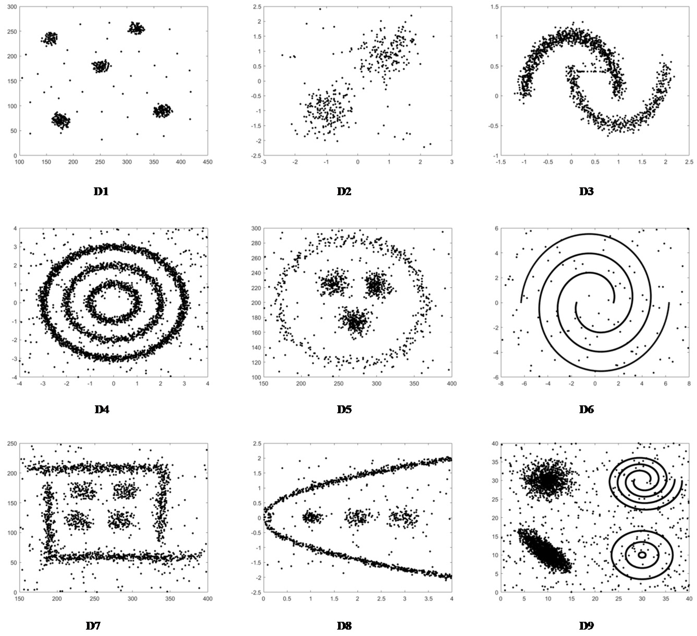
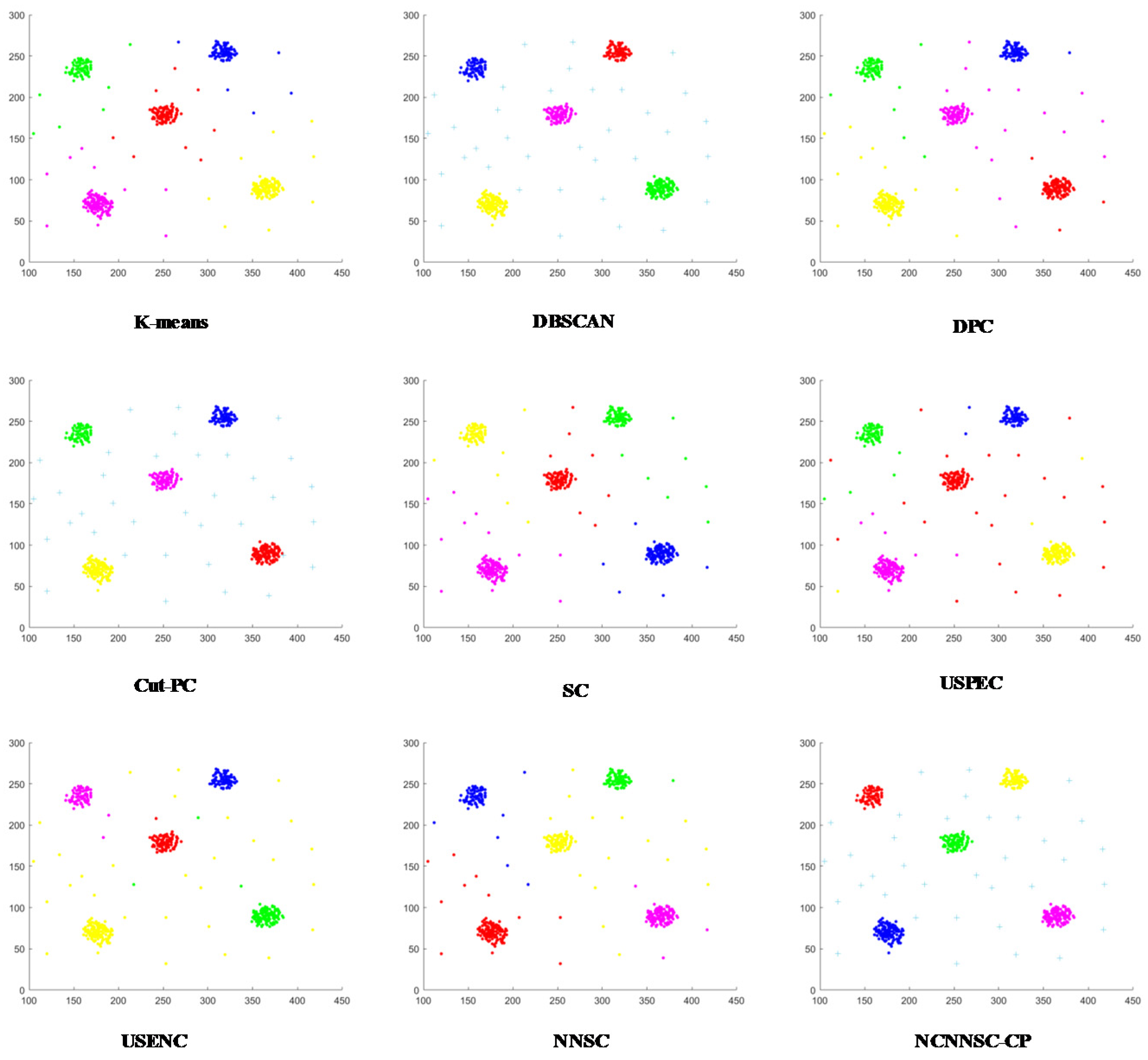
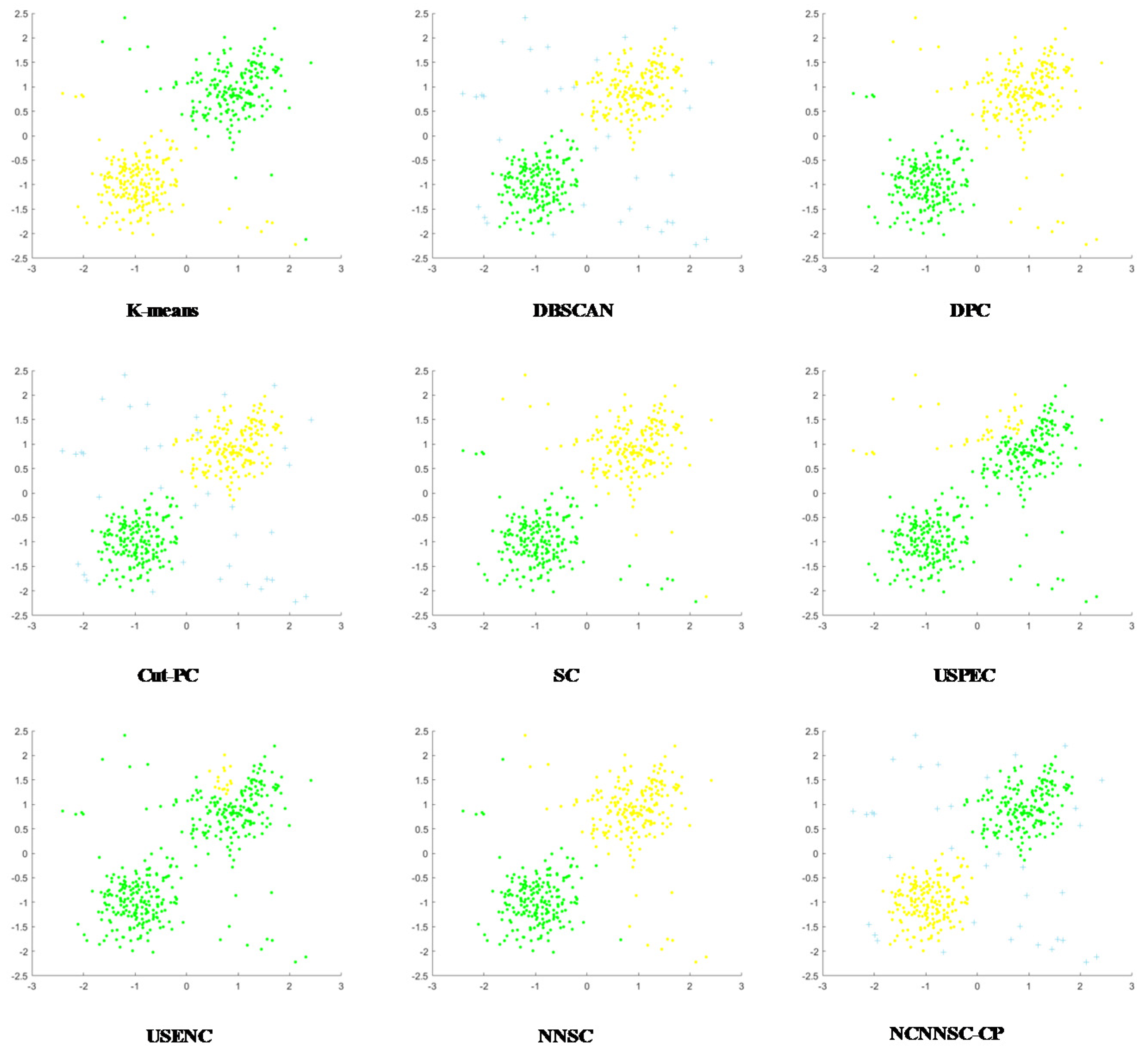
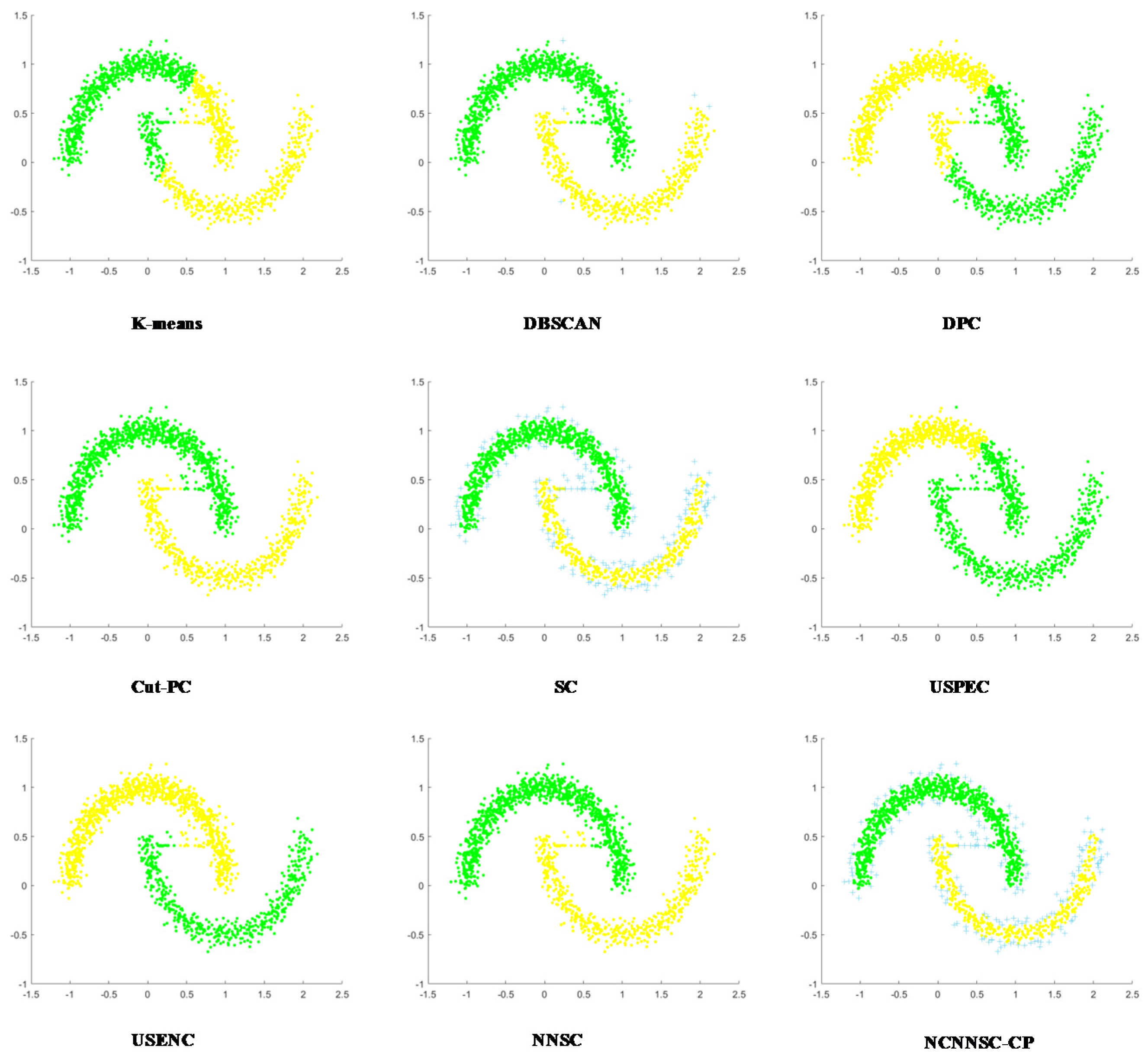
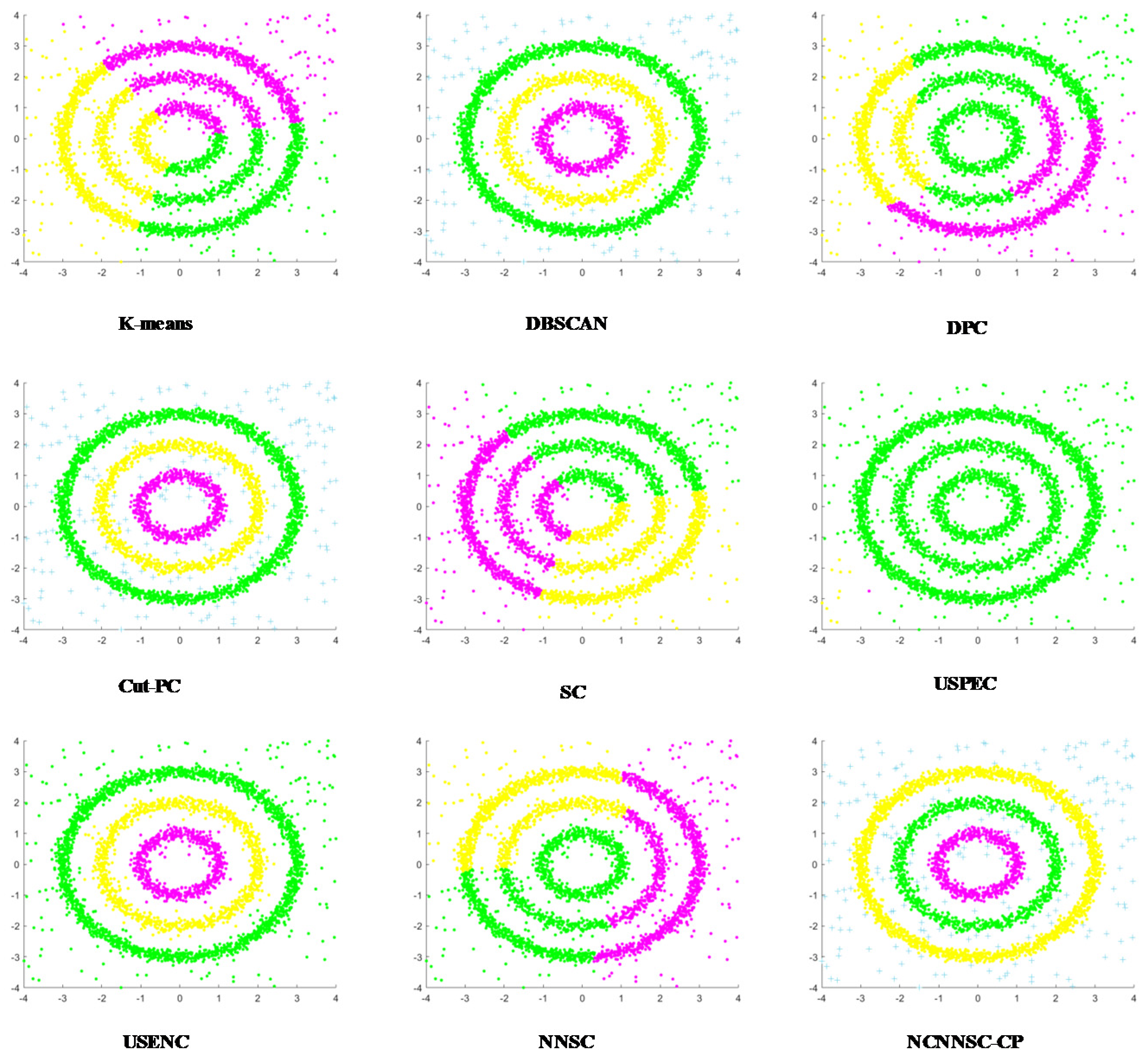
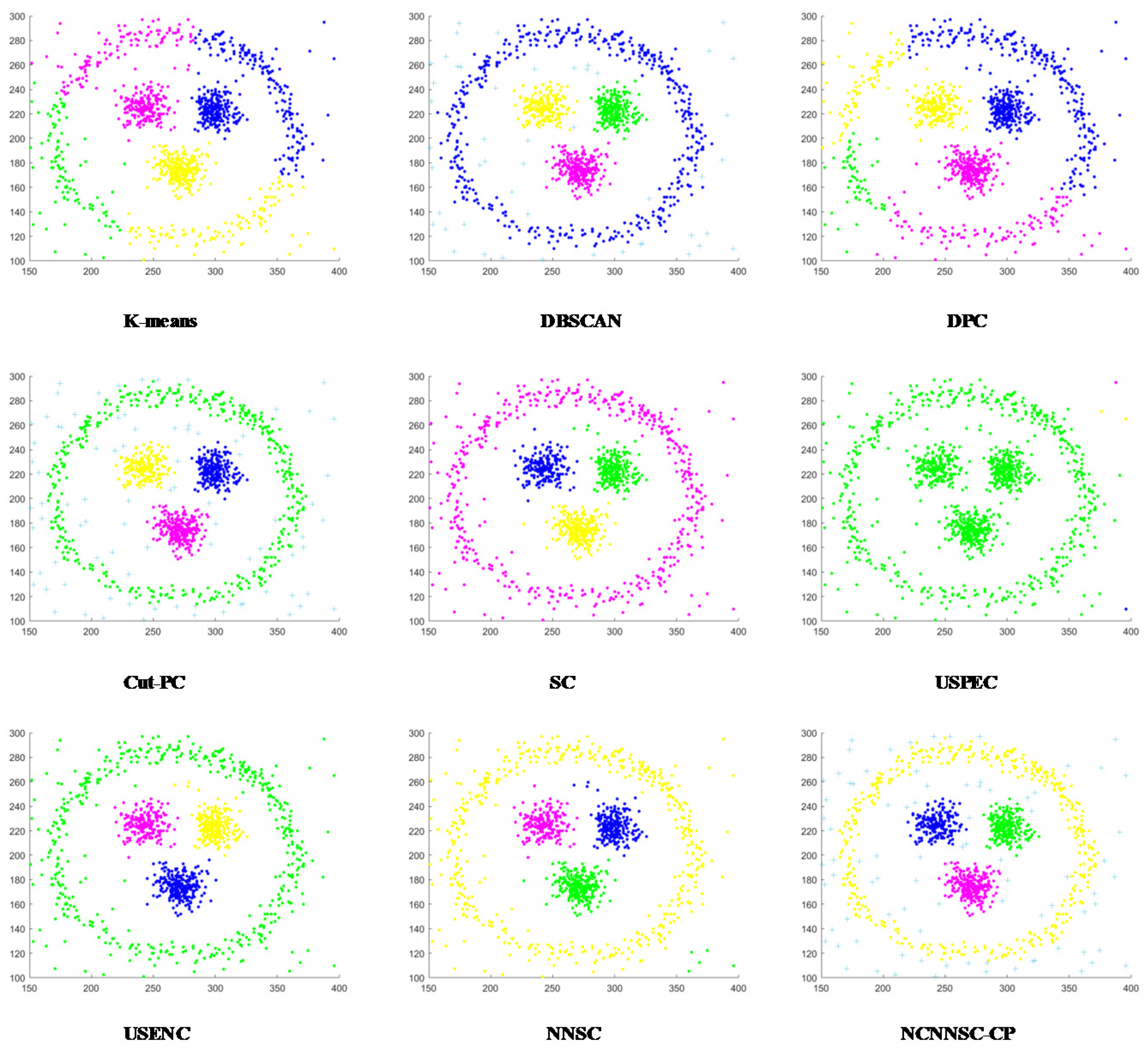
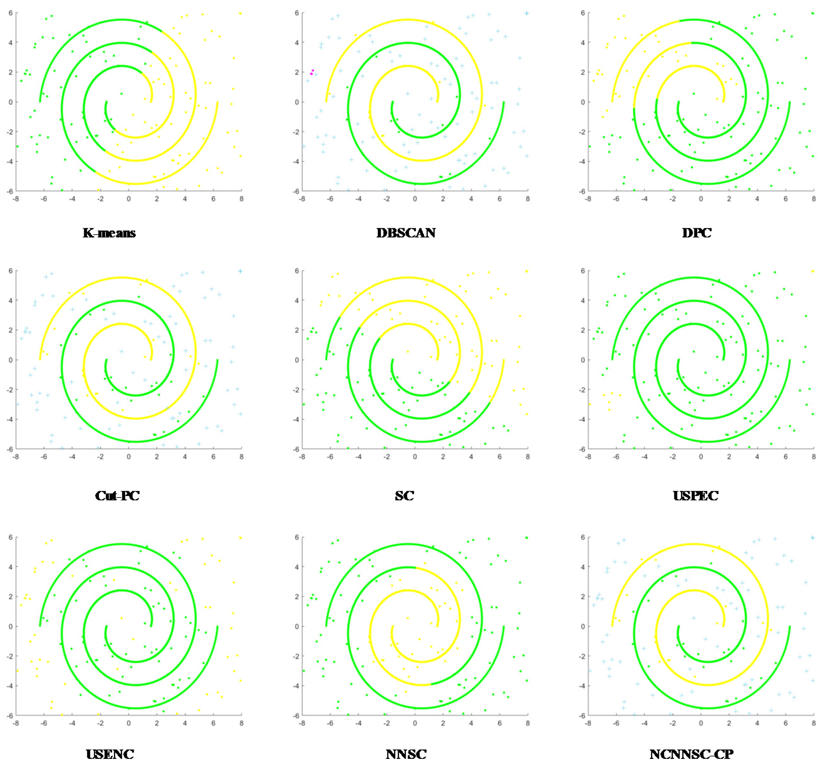
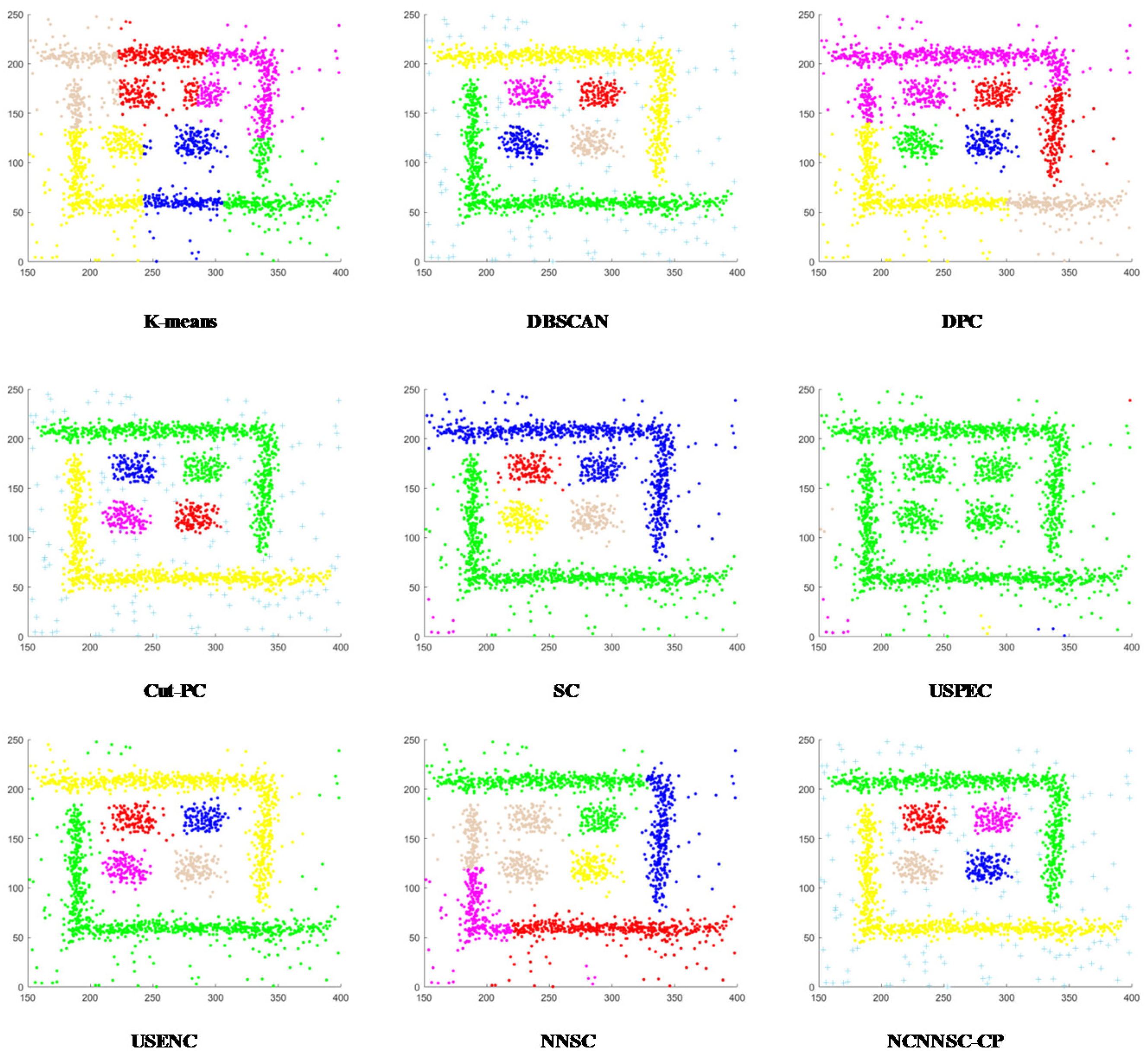
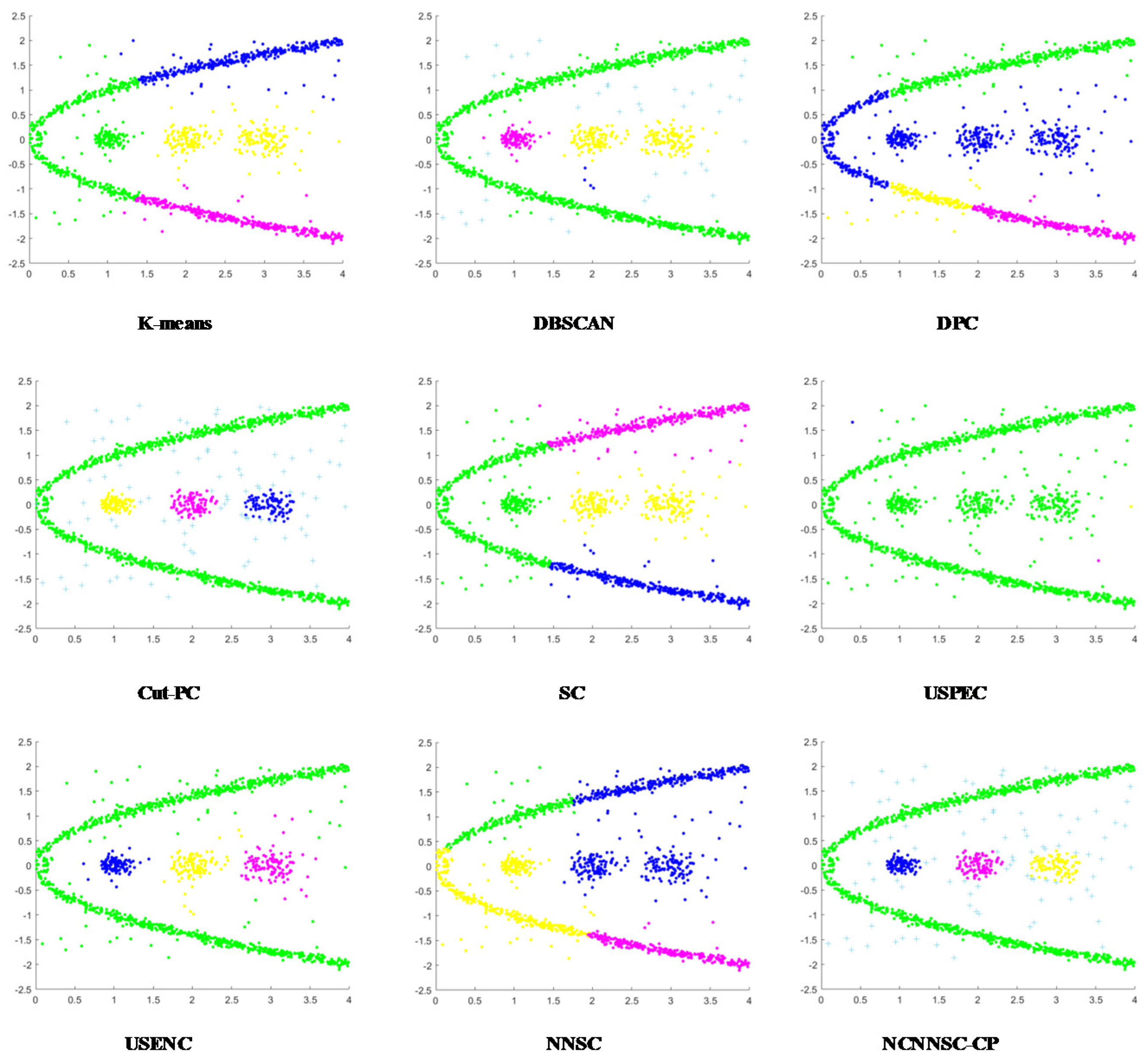
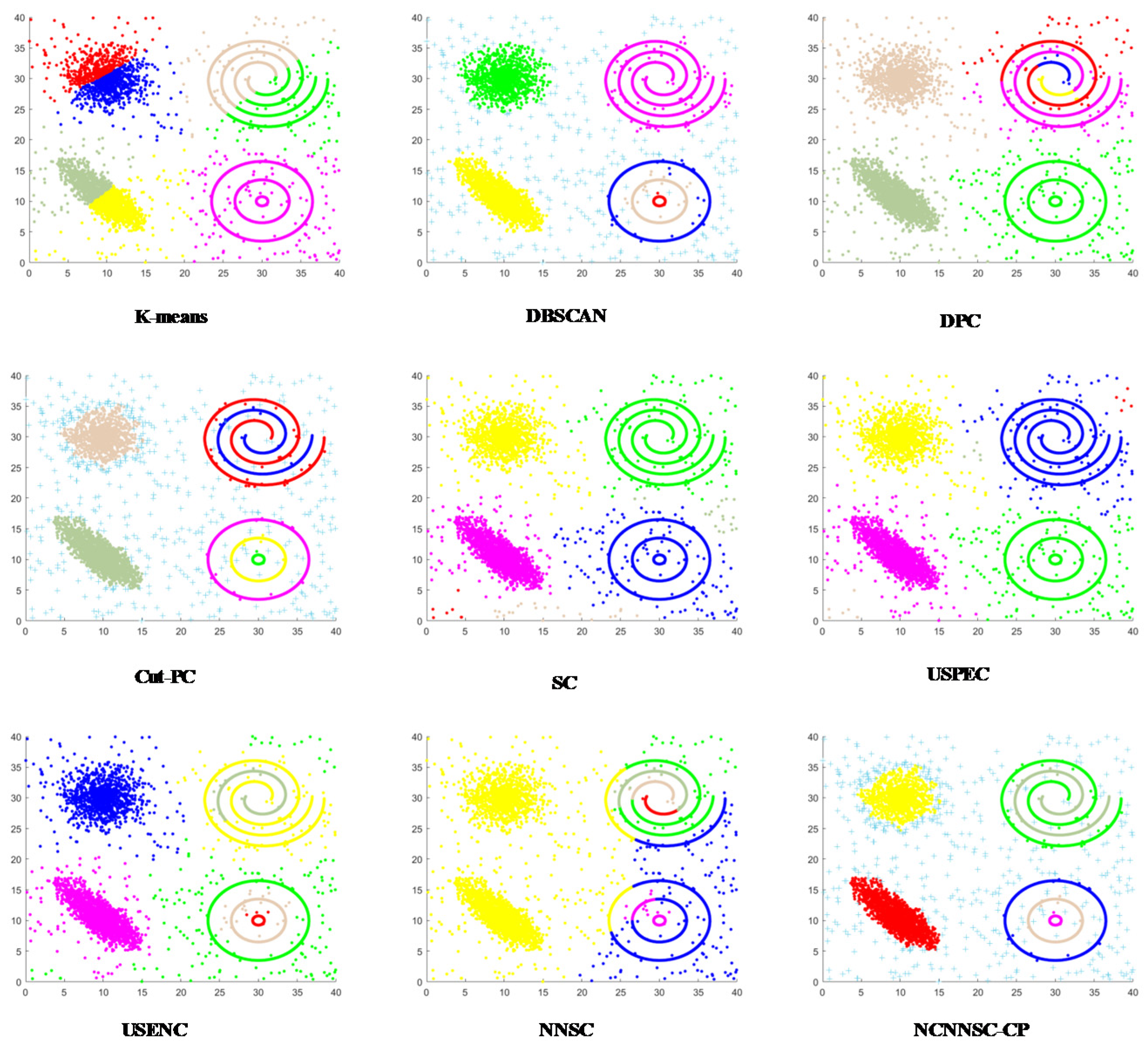
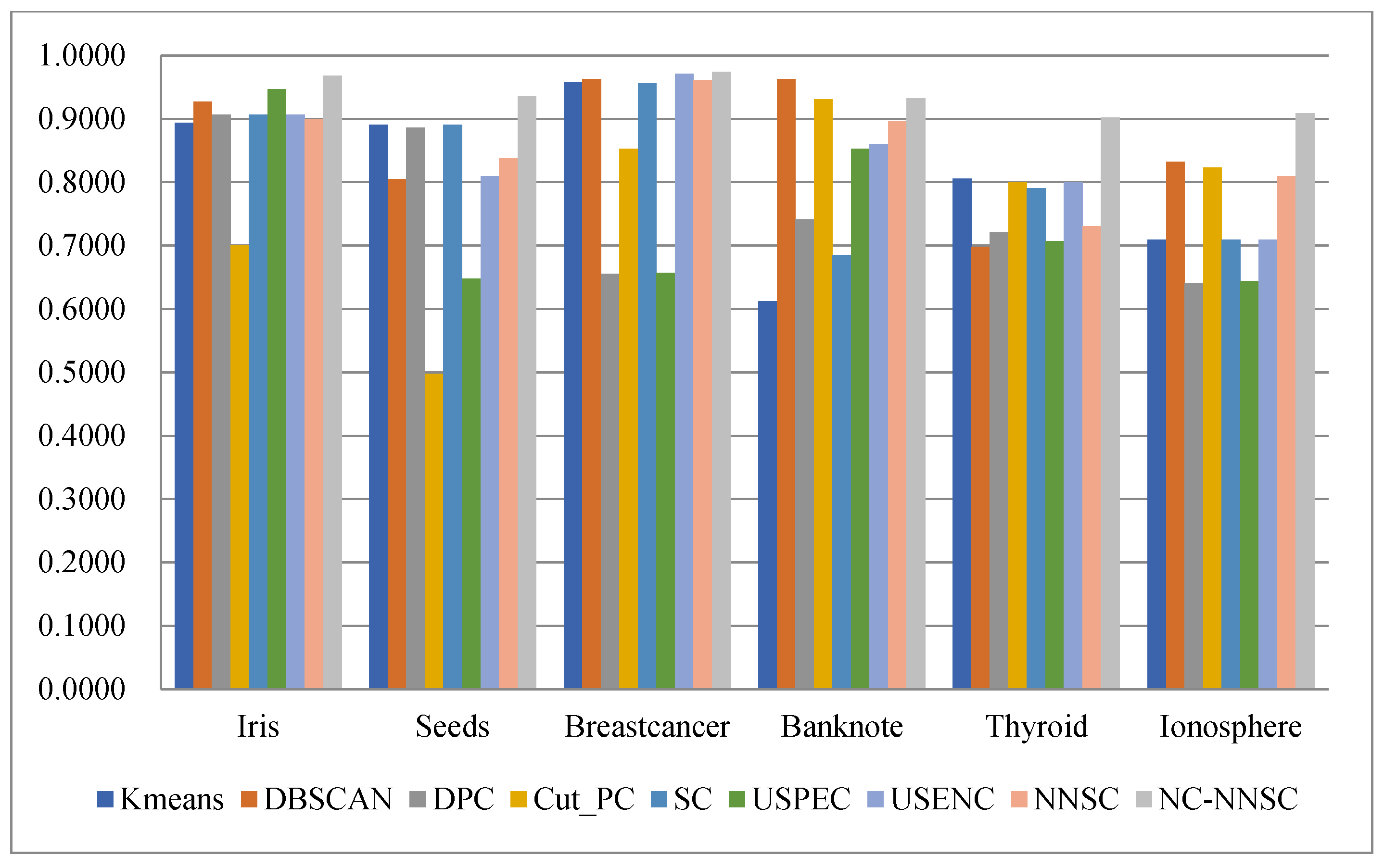
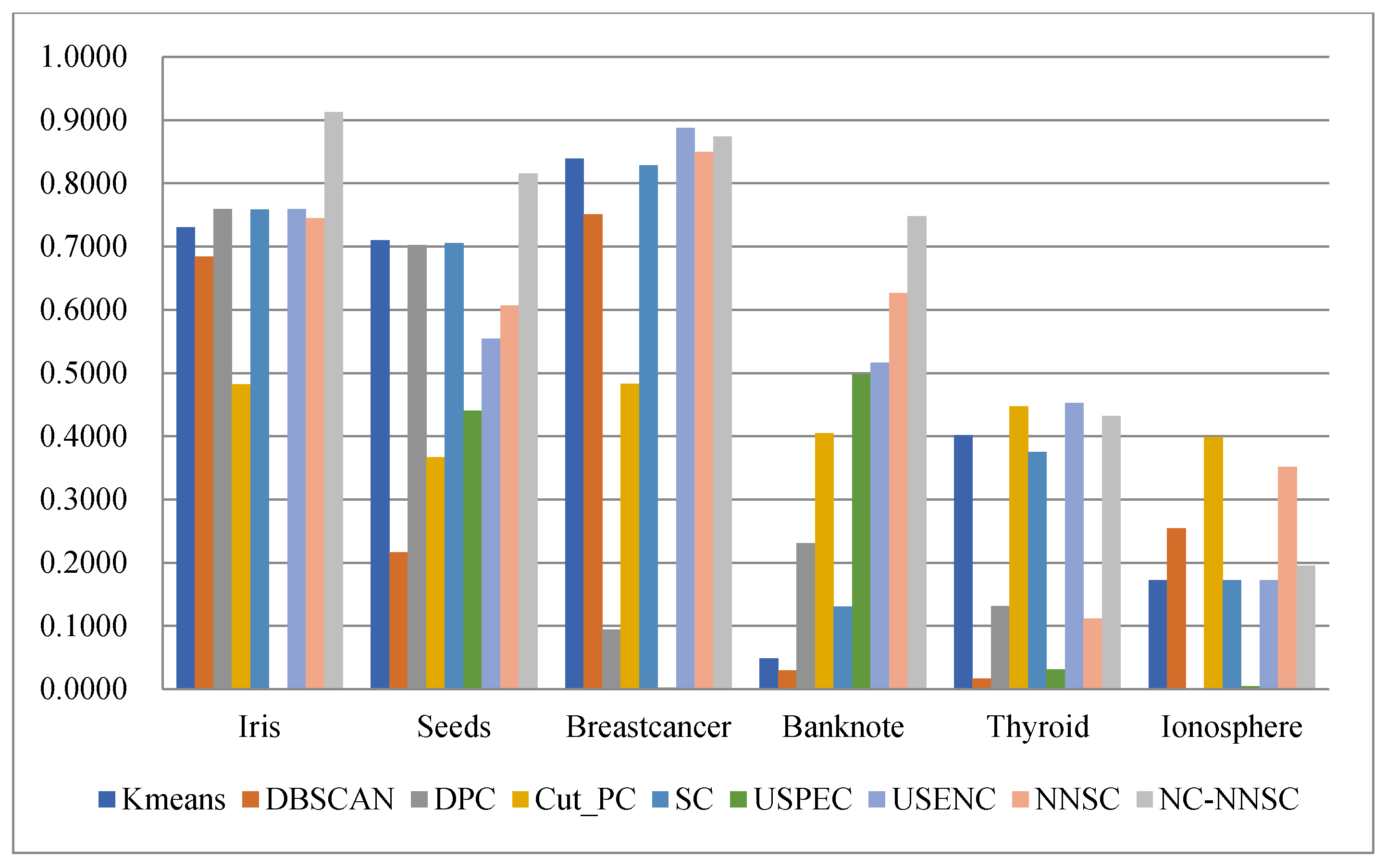
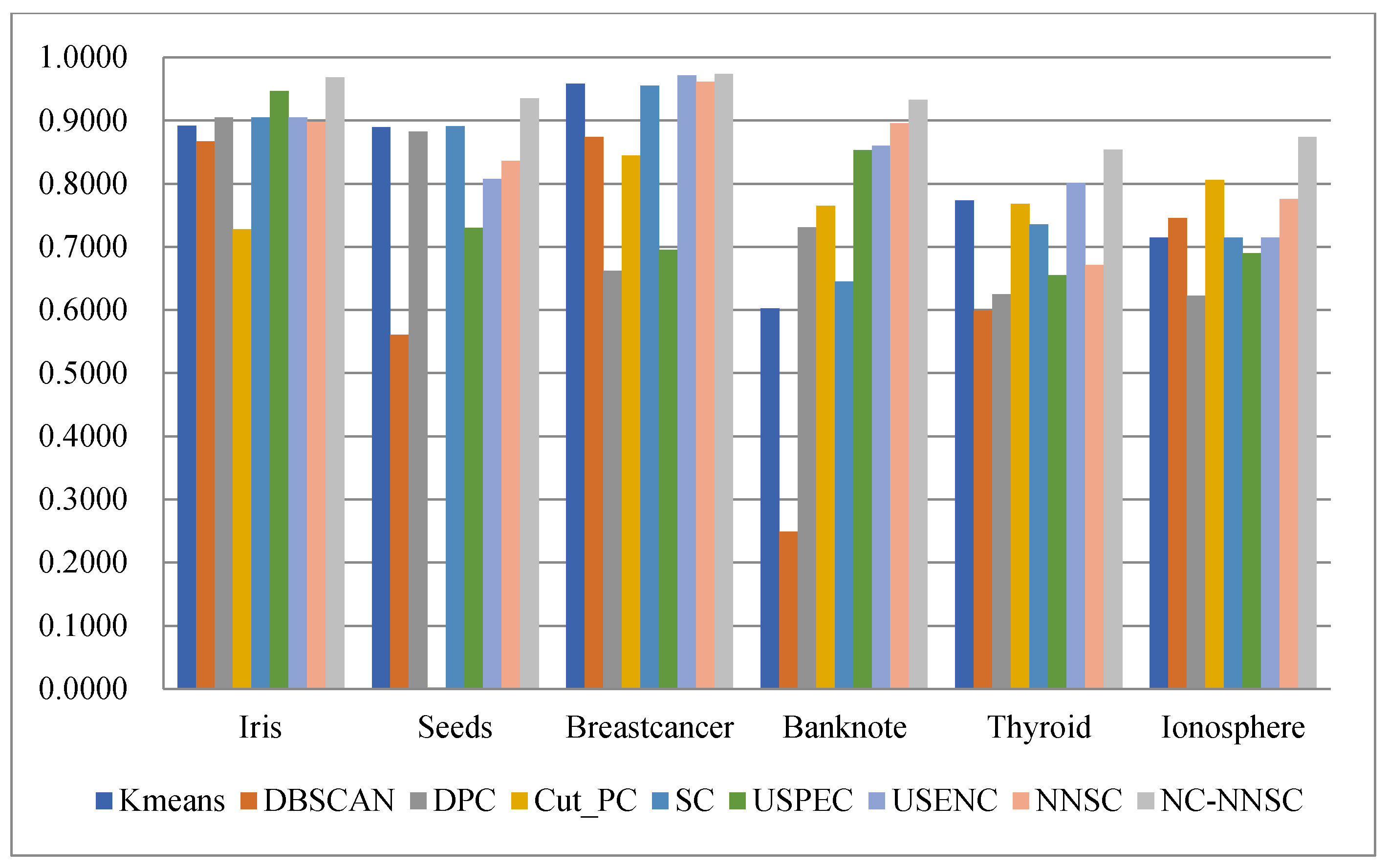
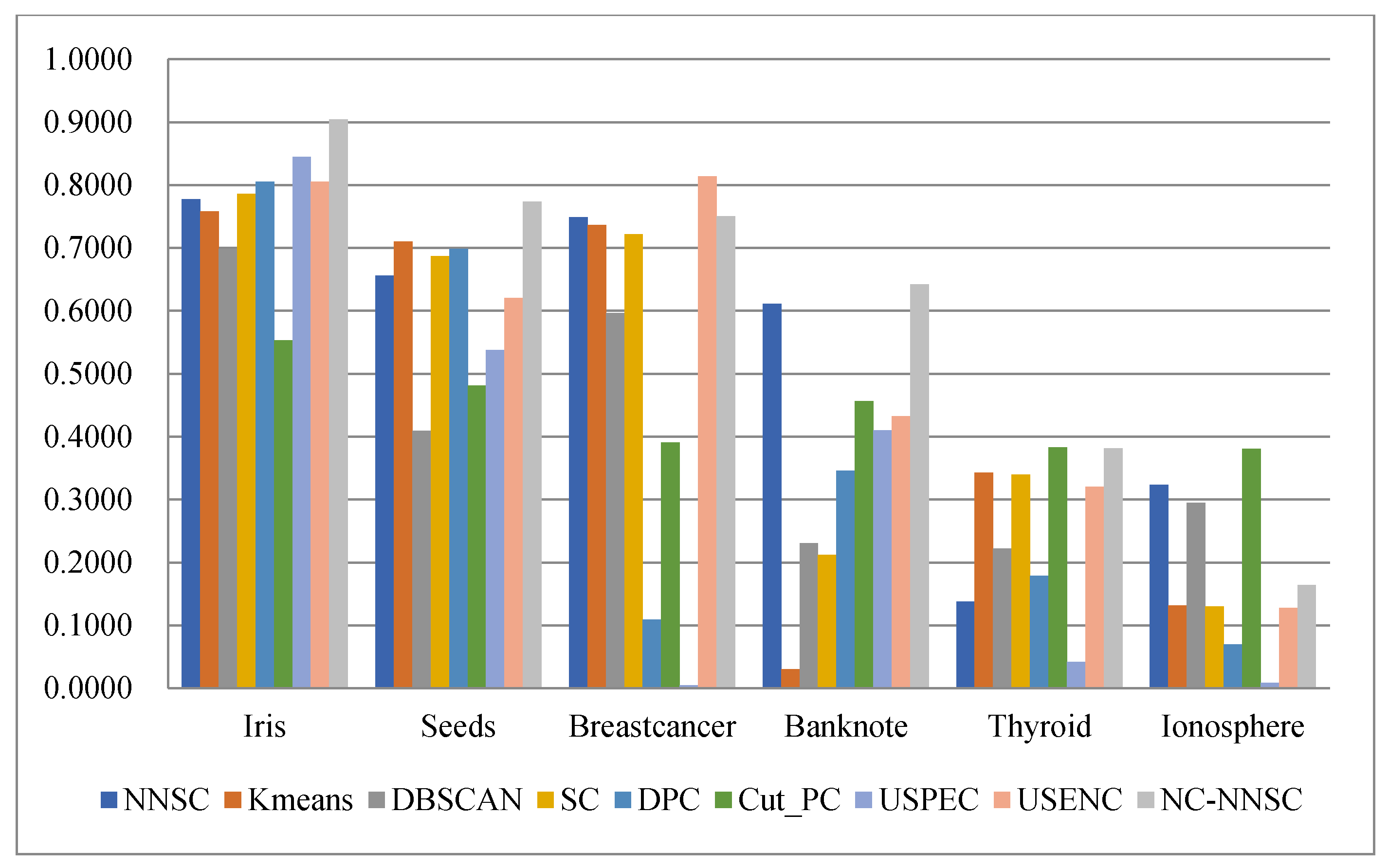
(4) Nine classical synthetic data sets and six UCI data sets are used to simulate and verify the clustering performances of NCNNSC-CP.
The rest of the paper is organized as follows.
Section 2 introduces the related concepts of P system and natural neighbors, and the basic algorithm of spectral clustering. In
Section 3, a spectral clustering method with noises cutting and natural neighbors based on the coupling P system is proposed.
Section 4 shows the performance of the algorithm through experimental analysis. Conclusions and future research work are given in
Section 5.
2. Related Work
2.1. Spectral Clustering
The spectral clustering algorithm is based on graph theory. Compared with traditional clustering algorithms, it can cluster data points with arbitrary shapes and converge to the global optimal solution efficiently. First, it constructs an undirected weighted graph based on similarity. Each of the graphs corresponds to a data point, and the weight is the similarity of the edges formed by the data points. Generally, there are three ways to construct an affinity matrix:
(1) -neighborhood graph. Set the distance threshold , Euclidean distance . , if ; otherwise, .
(2) K-nearest neighbor graph. Using the KNN algorithm obtains the k neighbors of each data point, only when is one of the k neighbors of , and .
(3) Fully connected graph. In general spectral clustering, it is the most commonly used method of constructing affinity matrix. Different kernel functions can be selected to define the weight between edges. When using Gaussian kernel function, the similarity matrix and the affinity matrix are the same, .
Then, according to the affinity matrix, we construct the degree matrix D. For any point in the graph, its degree is defined as the sum of the weights of all edges connected to it The most important process in spectral clustering is the construction of Laplacian matrix L:
(1) The denormalized Laplacian matrix
(2) Normalized Laplacian matrix based on Random Walk
(3) Symmetric normalized Laplacian matrix
Next, the eigenvector corresponding to the first k eigenvalues of the L can be calculated and set: . In addition, U is normalized by row to generate , and each row of Y represents a sample. At last, the clustering algorithm (such as k-means) is applied to cluster the new samples into clusters .
The basic spectral clustering algorithm (NJW) [
29] is shown in Algorithm 1.
| Algorithm 1 Spectral clustering (NJW) |
| Input: The dataset D |
| Output: C (the clustering results) |
| 1: Construct the affinity matrix W. |
| 2: Degree matrix D, |
| 3: Laplacian matrix |
| 4: Construct the feature matrix |
| 5: Form the matrix Y from U, |
| 6: C = K-means(Y) |
2.2. Natural Neighbors
Zhu [
30] systematically expounded the concept of natural neighbors through induction and summary based on previous studies, which is a reflection of the friendship between people in human society. Compared with the traditional nearest neighbor method, the natural neighbor method is scale-free. The relevant definitions of natural neighbors are as follows.
Definition 1: (The Natural Neighbor Stable Structure).The natural neighbor stable structure is, generally speaking, that A is a Natural Neighbor of B if A regards B as a neighbor and B regards A as a neighbor at the same time.where NNk(xi) is the kth nearest neighbor of point xi. Definition 2: (k-Nearest Neighbors).Given a data set D, for any point, its k nearest neighbors refer to a set of points in D with, which iswhereis the distance of the kth nearest neighbor of. Definition 3: (Reverse Neighbors).The reverse neighbor ofis considered to be a set of data points x in D that takeas its k nearest neighbor, which is Definition 4: (The Natural Characteristic Value Sup [31]).Sup is the search range in the natural neighbor method.where the initial value of k is 1, andis the number of reverse neighbors ofin the kth iteration. In addition, Definition 5: (The Natural Neighbors).For each object x in dataset D, its natural neighbors are k nearest neighbors, denoted as NaN (x).
2.3. Cell-Like and Tissue-Like P System
2.3.1. Cell-Like P System
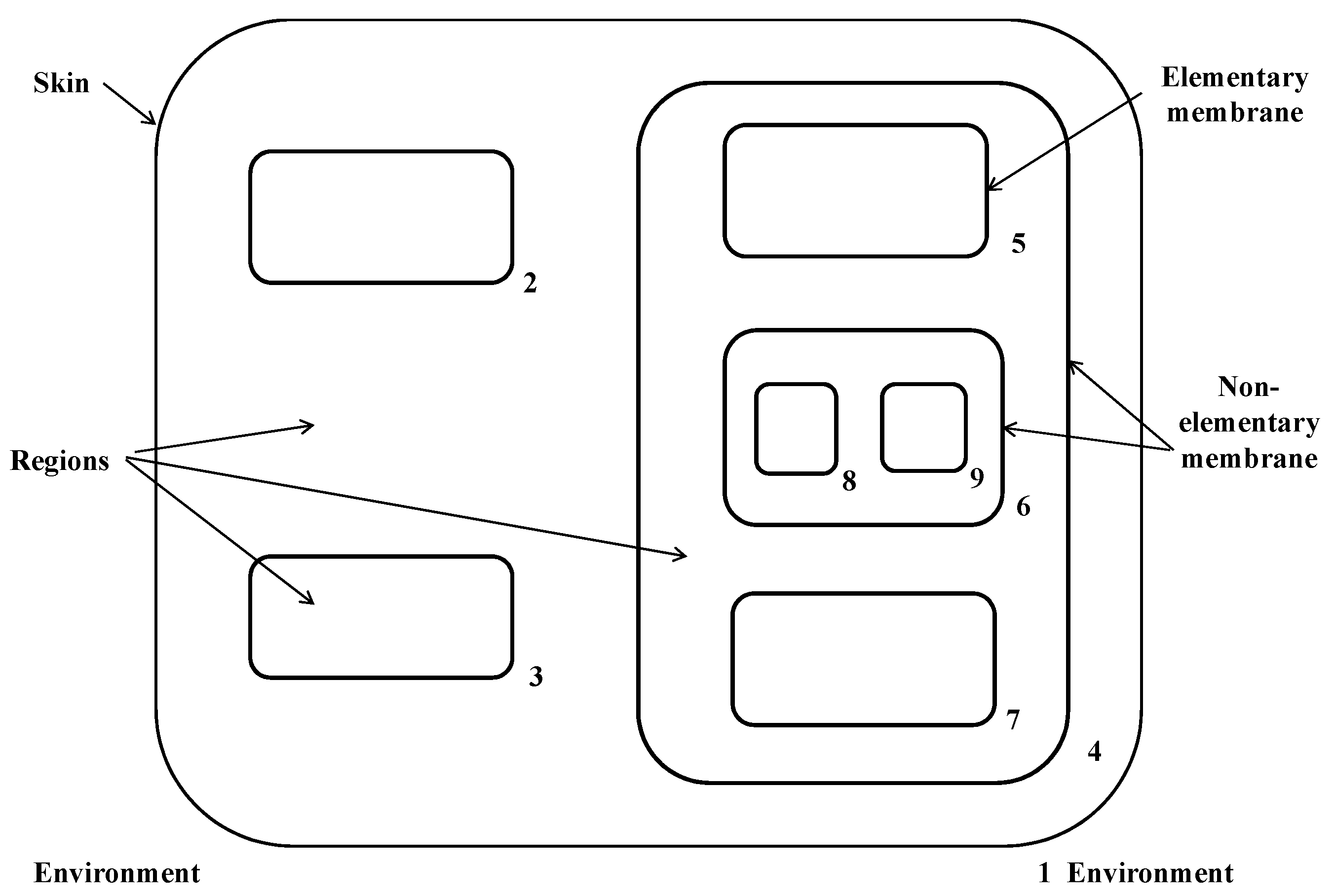
The cell-like P system is the first proposed P system, and its membrane structure is shown in
Figure 1. The outermost membrane 1 is the skin membrane. The skin membrane separates the entire P system from the external environment. If a membrane does not contain a submembrane inside, the membrane is a basic membrane (such as membrane s2, 3, 5, 8, 9, and 7). Otherwise, it is called a non-basic membrane (such as membranes 1, 4, and 6).
The formal definition of the cell-like P system is
where
O is the alphabet, where the elements represent objects;
H is a collection of membrane labels;
represents the membrane structure;
refers to the multiple set of objects contained in region in the membrane structure;
R contains all the rules;
represents the input/output area of the system, where e is a reserved character not included in H.
Given a P system, that is, given the membrane structure, the simplified objects of each membrane area and the corresponding rules. Each process of the P system is an execution rule of non-determinism and maximum parallelism. After each time step, the system enters a new pattern.
2.3.2. Tissue-Like P System
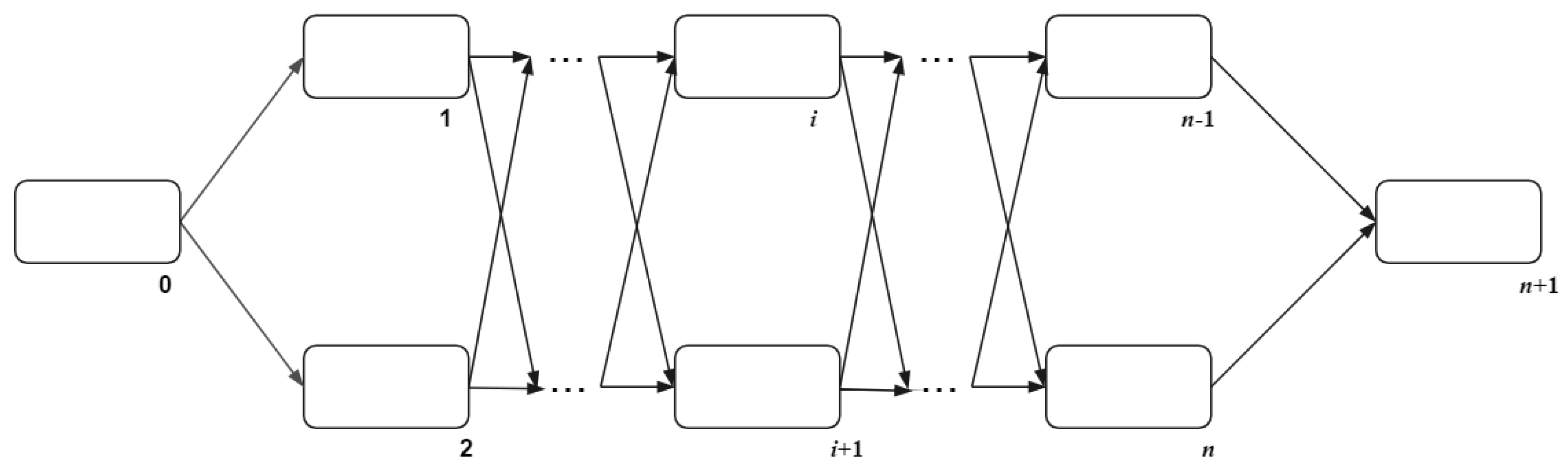
The tissue-like P system regards cells as the vertices of the graph in the system. The cells in the P system have different states, and the rules can be executed only when the required states are met. The basic membrane structure of the tissue-like P system is shown in
Figure 2. Cell 0 is the input cell, which contains the initial object. The initial object uses rules and communication mechanisms to communicate in cell 1 to cell
n. Cell
n + 1 is the output cell, used to store the obtained results.
The formal definition of the traditional tissue-like P system is
where
O is the alphabet, which contains all objects in the system;
are synapses that connects cells;
indicates the output cells of the system;
represents n cells in the system, the detail definition are as follows:
where
- (1)
shows the collection of all states;
- (2)
refers to the initial state;
- (3)
indicates the initial multiset of the object, when , there is no object in cell i;
- (4)
stands for the rules of the entire system.
3. Noises Cutting and Natural Neighbors Spectral Clustering Based on Coupling P System
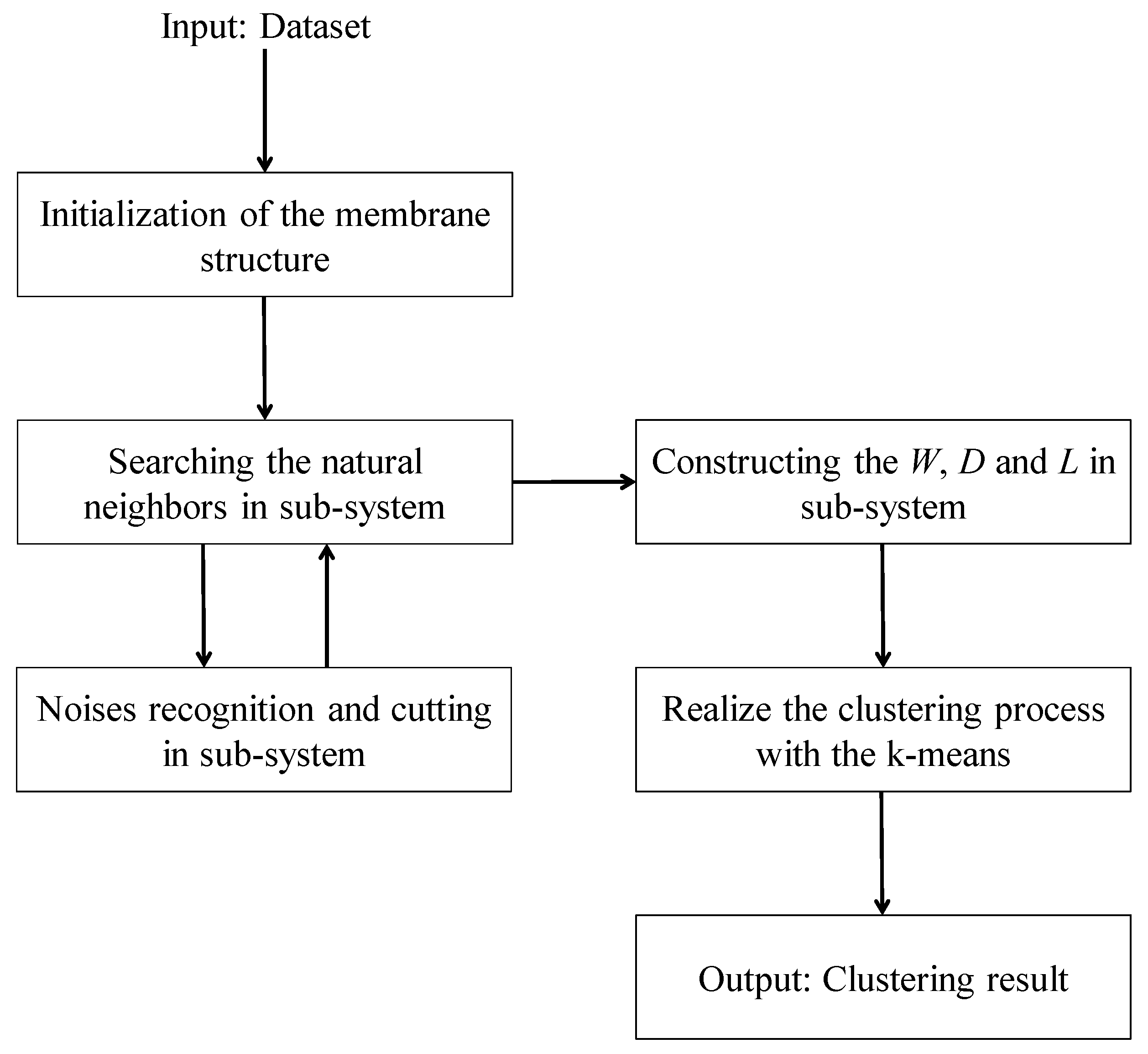
In this section, the spectral clustering method with noises cutting and the natural neighbors based on coupling P system is proposed. First, we explain the general framework of the coupling P system. Then, the different evolution rules and operations in the subsystems such as searching the natural neighbors, noises cutting, constructing affinity matrix, and clustering are introduced, respectively. Meanwhile, the communication rules between different membranes are elaborated. The flow chart of the proposed
NCNNSC-CP algorithm is shown in
Figure 3.
3.1. The General Framework of the Coupling P System
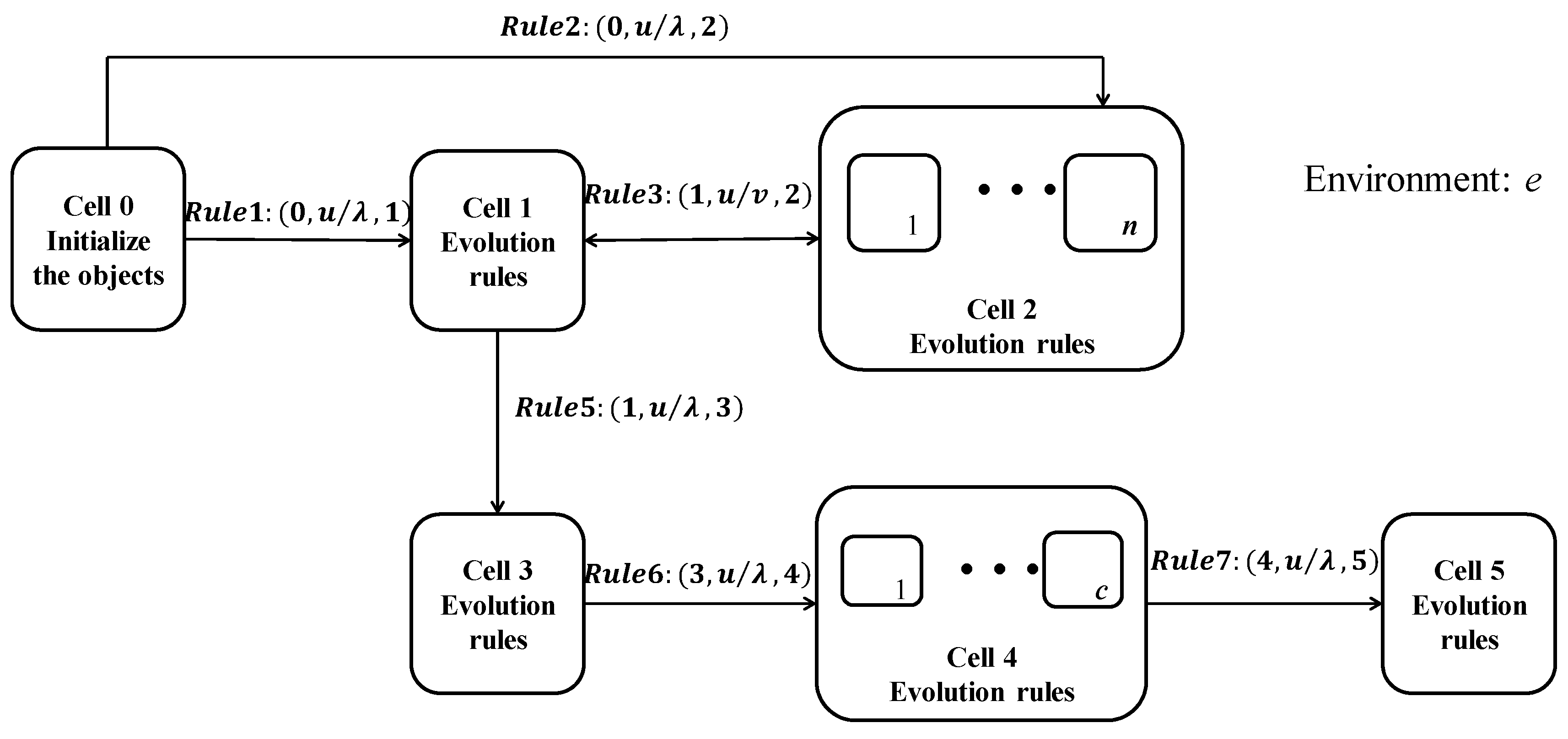
The proposed coupled P system (
NCNNSC-CP) is the coupling of the cell-like P system and the tissue-like P system. According to the related concepts introduced in
Section 2.3, the basic structure of the coupled P system is shown in
Figure 4.
The formal definition of the coupled P system is
where
. xi represents each data point. dij represents the distance between arbitrary two points. The natural neighbors of x denoted as NaN (x). Nb(x) refers to the number of reverse neighbors of x. Sup is the natural characteristic value. Noises stand for the noisy points in the dataset. c is the number of clusters. The similarity between data points xi and xj represented by wij. Dii indicates the degree of data point xi. L represents the Laplace matrix. is the tuning parameters parameter.
represents the initial objects in the system.
stands for the structure of the membrane.
Syn = {{0,1},{0,2},{1,2}{1,3},{2,1},{3,4},{4,5}} means the synapses between cells. Its main function is to link cells so that they can communicate with each other.
in is cell 0, the input membrane. out is cell 5, the output membrane.
refers to cells in the system. The m is determined according to the number of clusters and the number of data points.
R is the collection of rules, including communication rules and evolution rules.
Evolution rules are used to modify objects in the cluster, and communication rules are used to transfer objects from one cell to another.
3.2. The Evolution Rules
The rule
R0 for inputting cell is to transfer the raw dataset and the parameters to cell 1 for subsequent clustering algorithm operations. At the same time, the original data are transmitted to the cell 2 to perform noise cutting on the original data after the noises recognition. The specific
R0 rules can be described as
In terms of output cell 5, it is mainly used to store clustering results .
3.2.1. The Evolution Rules of Searching the Natural Neighbors in Cell 1
The construction of affinity matrix can directly affect the clustering results of spectral clustering. In traditional algorithms, most of the parameters are determined based on artificial experience and manually input. According to the related concepts of natural neighbors and membrane system in
Section 2, this paper uses the rules of searching natural neighbors without parameters in the membrane system to determine the natural characteristic value
Sup and natural neighbors
NaN(
x).
In summary, the details rules of the evolution rules of The Natural Neighbors Searching (NaN-searching) in cell 1 are shown in rules R1.
R11 (Sorting rule): Create a KD-tree T from the dataset D, which calculates the Euclidean distance of all points in the dataset D, and then sorts them in ascending order.
R12 (Searching rule): For each point xi in D, we use a KD-tree T to find its rth neighbor xj.
Then, Nb(xj) = Nb(xi) + 1, according to Definition 2, Definition 3, and Equations (2) and (3) in cell 1. Finally, the natural neighbors of each point NaN(x) are transmitted to cell 2.
R13 (Iteration stop rule): When the number of xi’s reverse neighbors Nb(xi) no longer changes or is always equal to 0, evolution stops.
R14 (Determining the natural characteristic value Sup rule): the natural characteristic value Sup is calculated by Equation (4) in the cell 1. Then, transmitted the Sup to cell 2.
Apparently, the search of natural neighbors is different from the traditional k-nearest method. The k nearest neighbors of each point xi can be found without any parameters in the whole algorithm process in cell 1.
3.2.2. The Evolution Rules of Noises Recognition and Cutting in Cell 2
In cell 2, we execute the evolutionary rules of noises recognition and cutting.
Noise points refer to data with errors or anomalies (deviations from expected values) in the data, which are neither core points nor boundary points in the data set. At the same time, these noises cause great interference to the data analysis and preprocessing, especially for clustering, which is extremely sensitive to them based on empirical data. Therefore, it is particularly significant to identify and eliminate noise points. Jokinen et al. [
6] deal with noise on the basis of spatial clustering based on hierarchical density, and proposes a density-based cluster ability measure. We propose a noise recognition and cutting method based on the reverse density and critical reverse density in natural neighbors. The reverse density and critical reverse density are specifically defined as follows.
Definition 6: (Reverse density).Based on the natural neighbors NaN(xi) of the data object xi, we define the inverse density as the average distance between xi and all its natural neighbors: Definition 7: (Critical Reverse density).The critical reverse density of point xi is calculated from the average reverse density Rd(xi) and the standard deviation of the reverse density std(Rd(xi)) of all objects in the data set D:whereis a tuning coefficient, and experiments show that a = 1 is suitable for most data sets. Definition 8: (Noises).If the xi’s reverse density is larger than its critical inverse density, it is a noise point. In accordance with the natural neighbors of point x obtained in cell 1 and the above concepts, we simultaneously conduct noise recognition for all points in the n sub-cells of cell 2. This step is parallel to improve computational efficiency. When it is judged that x is a noise, it is transported to the environment outside the cell 2 and discard x. The details rules of the evolution rules of Noises Recognition and Cutting (Noises-rc) in cell 2 are shown in rules R2.
R21 (Noise recognition rule): For each point xi in D, using Equation (6) to get Rd(x) and then using Equation (7) to get CRd(x) in sub-cells of cell 2.
R22 (Noise cutting rule): For each point xi in D, if the object xi satisfies the Equation (8) it will be transmitted from the cell 2 to the environment. Otherwise, the rest of the data is sent to cell 1.
3.2.3. The Evolution Rules of Constructing the Affinity Matrix, Degree Matrix and Laplacian Matrix in Cell 3
In spectral clustering, the construction of affinity matrix plays an important role in the clustering result. Generally, it is obtained by calculating the Gaussian kernel distance between the data point
xi and its natural neighbors. However, due to the influence of noise points, the natural neighbors of the data points are mixed with noises, which is not conducive to the construction of the affinity matrix. Relatively speaking, noise identification and screening based on reverse density and critical reverse density are extremely effective. The data set
D’ is deduced through the
Section 3.2.2 which is the core data set. Therefore, we perform the natural neighbor searching again to acquire the core natural neighbor of the data object. Although it will increase the complexity of the algorithm to a certain extent, it is worthwhile compared with the greatly improved accuracy. The core natural neighbor is defined as follows.
Definition 9: (The Core Natural Neighbors).For each object x in dataset D, its core natural neighbors are k nearest neighbors without noises, denoted as CNaN (x).
At last, we perform spectral clustering (NJW [
28]). On the basis of the affinity matrix
W, we calculate the degree matrix
D:
As for the Laplacian matrix
L, we utilize the Symmetric normalized Laplacian matrix:
Next, we choose the eigenvector
corresponding to the first
k eigenvalues of the
L to comprise
, and standardize it by row to get
Y:
The details rules of the evolution rules of constructing the Affinity Matrix, Degree Matrix, and Laplace matrix in cell 3 are shown in rules R3.
R31 (Constructing the affinity matrix rule): Based on the core natural neighbors CNaN (x) and the input parameters, the affinity matrix W is calculated in cell 3. For the jth natural neighbor in CNaN(xi) of xi, . Moreover, If Wij is a real number while Wji is equal to 0, the value of Wij is assigned to Wji by the principle of symmetry.
R32 (Constructing the degree matrix rule): According as the affinity matrix and the Equation (8), the degree matrix is obtained in cell 3.
R33 (Constructing the Laplacian matrix rule): As for the Laplacian matrix L, we utilize the Symmetric normalized Laplacian matrix using Equation (9) in cell 3.
R34 (Constructing novel cluster sample): Based on the above concepts and Equation (10), we construct the Y in cell 3 for the next step of clustering. Each row of Y represents a sample. Simultaneously, it is transmitted into cell 4.
3.2.4. The Evolution Rules of K-Means (Clustering Method)
In the last step of NCNNSC-CP, the K-means is applied to cluster the new samples into clusters . In cell 4, there are k sub-cells running simultaneously.
The details rules of the evolution rules of K-means are shown in rules R4.
R41 (Random selection of cluster center rule): Randomly selecting c points from the dataset as the initial cluster centers and store them in c sub-cells.
R42 (Clustering rule): The distance between each sample point and each cluster center in sub-cell is calculated and transmitted to cell 4. Then, the data points are clustered according to the principle of nearest distance in cell 4.
R43 (Redefine the cluster center rule): According to each cluster divided by rule R42, the average distance of each cluster is calculated to change the cluster center. If the cluster center changes, the clustering process are repeated. Otherwise, the cluster result is output to cell 5.
3.3. The Communication Rules between Different Cells
Communication between cells in the CP system can only be achieved when there is a synapse between different cells. In order to ensure the effectiveness of the system and improve the efficiency of the system, this paper constructs a CP system with directional communication rules. In the CP system, some membranes are responsible for initializing objects and outputting results, and some membranes are responsible for algorithm execution. Orderly communication between different membranes makes the whole algorithm more effective.
There are three communication rules in the CP system: one-way transmission and two-way transmission between cells and one-way transmission between cells and the environment.
(1) One-way transmission between cells includes Rule1, Rule2, Rule5, Rule6, and Rule7. is null.
It can transfer the string u including the original data and parameters from cell 0 to cell 1.
The original data string u can be sent to cell 2 from cell 1It can transfer the string u including the original data and parameter from cell 0 to cell 2.
It can transmit the strings u of the natural neighbors, natural characteristic value, and related parameter strings of the dataset in cell 1 to cell 3.
The strings u of new sample data and related parameter generated in cell 3 are transported to cell 4.
The clustering results generated in cell 4 are transferred to cell 5 for storage.
(2) Two-way transmission between cells is Rule3.
It can transfer the string u of the natural neighbors and the natural characteristic in cell 2 to cell 3, and transfer the dataset without noises υ in cell 3 to cell 2.
(3) One-way transmission between cell and the environment is Rule4.
3.4. Computational Complexity
We assume that n is the total number of points in the dataset. The time complexity of NCNNSC-CP algorithm can be calculated as follows. (1) The time complexity for searching the natural neighbors is O(nlogn). (2) Noise recognition and cutting require O(n). (3) Constructing the Affinity Matrix requires O(n2). (4) Eigenvalue decomposition requires O(n3). (5) Clustering by K-means requires O(n). To sum up, the overall complexity of the proposed clustering method NCNNSC-CP is O(n3).


