
Dynamic Model for Biomass and Proteins Production by Three Bacillus Thuringiensis ssp Kurstaki Strains

 , and
, and
Abstract
:1. Introduction
2. Materials and Methods
2.1. Microorganism and Culture Media
2.2. Inoculum Preparation
2.3. Culture Conditions
2.4. Analysis and Sampling Strategy
2.4.1. Detection of Sporulation
2.4.2. Biomass Analyses
Cells and Spores Counts
Cell Dry Weight
Quantification of Proteins Production
Sugar Analysis
2.5. Experimental Data
2.5.1. Btk. BLB1 Strain
2.5.2. Btk. HD1 Strain
2.5.3. Btk. LIP Strain
2.5.4. Model Assumptions
3. Results
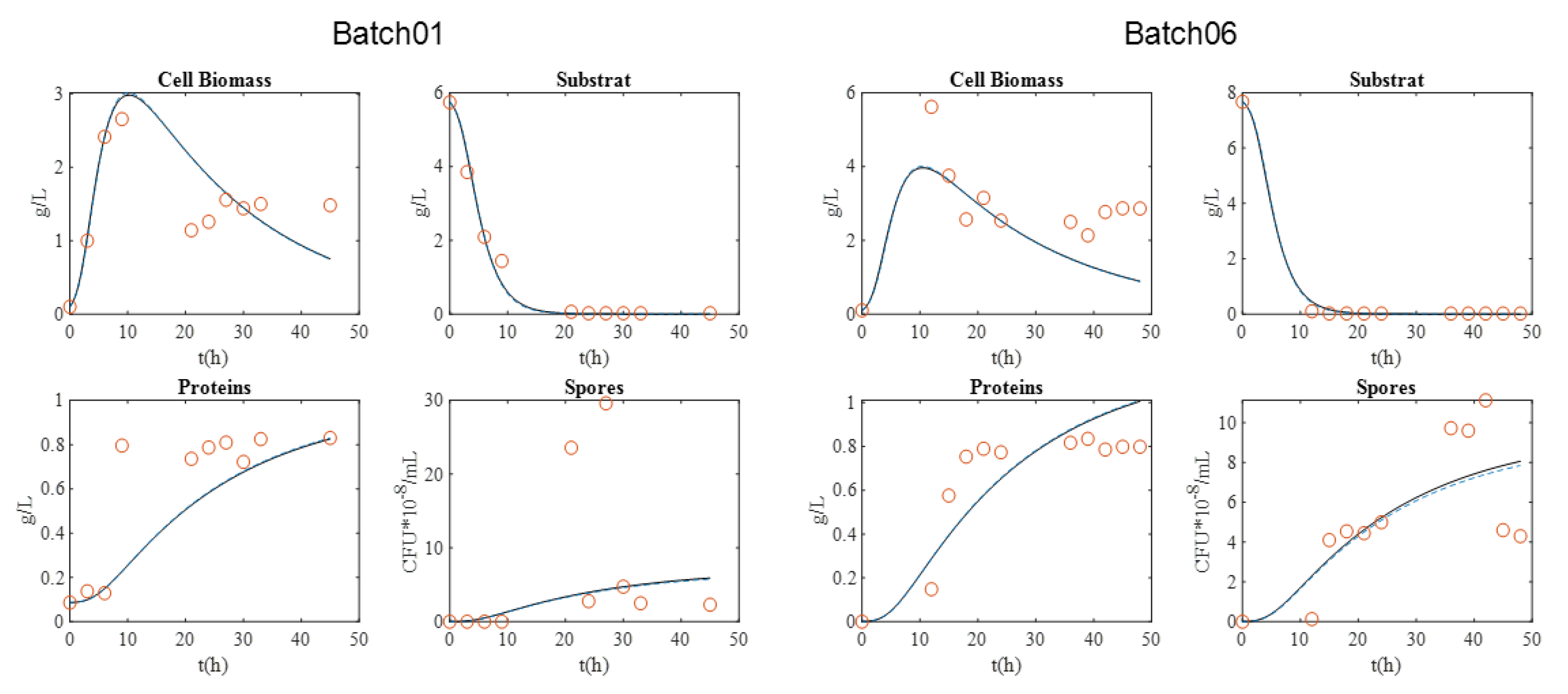
3.1. Model Calibration BLB1 Strain
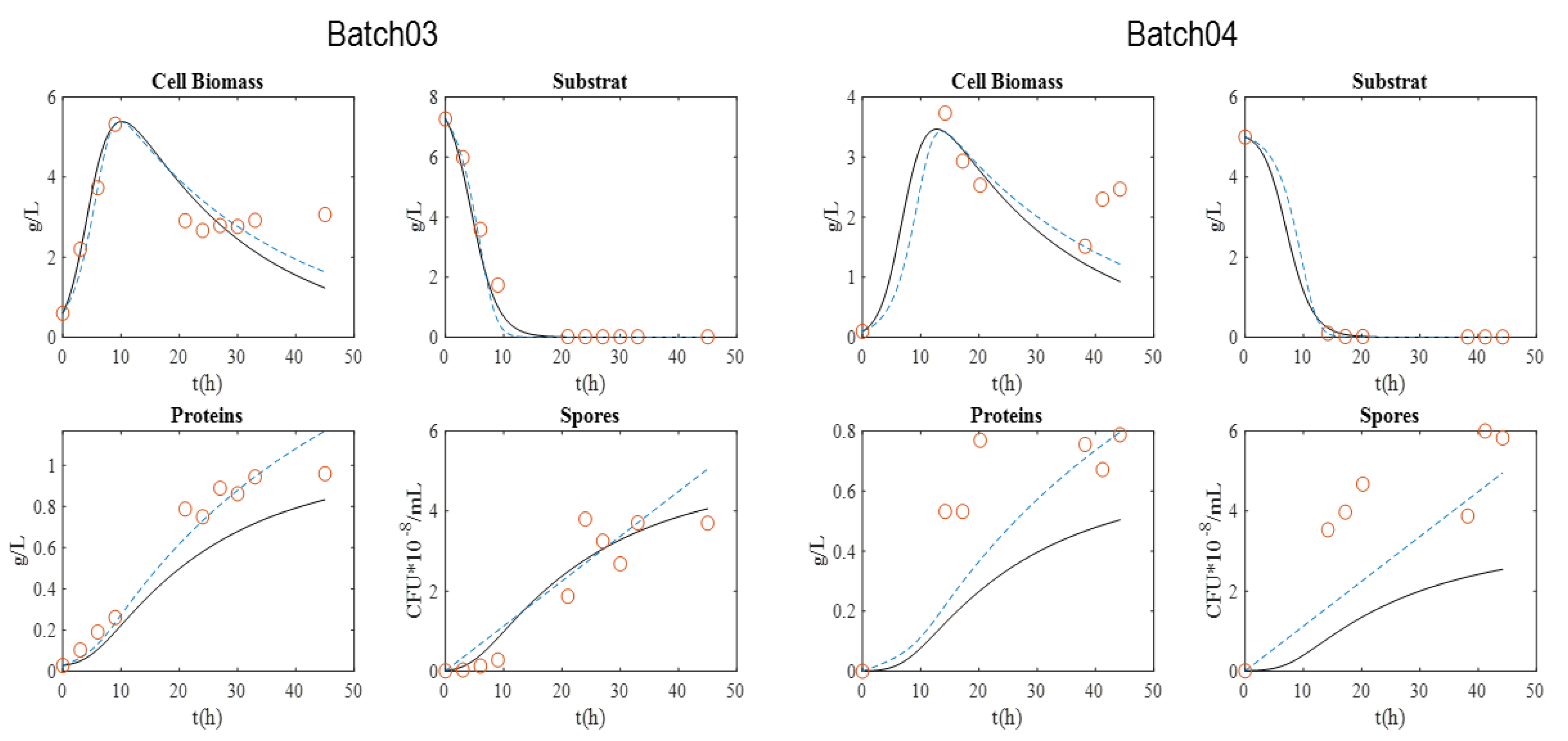
3.2. Model Calibration HD1 Strain
3.3. Model Calibration LIP Strain
3.4. Model Validation
3.4.1. BLB1 Strain
3.4.2. HD1 Strain
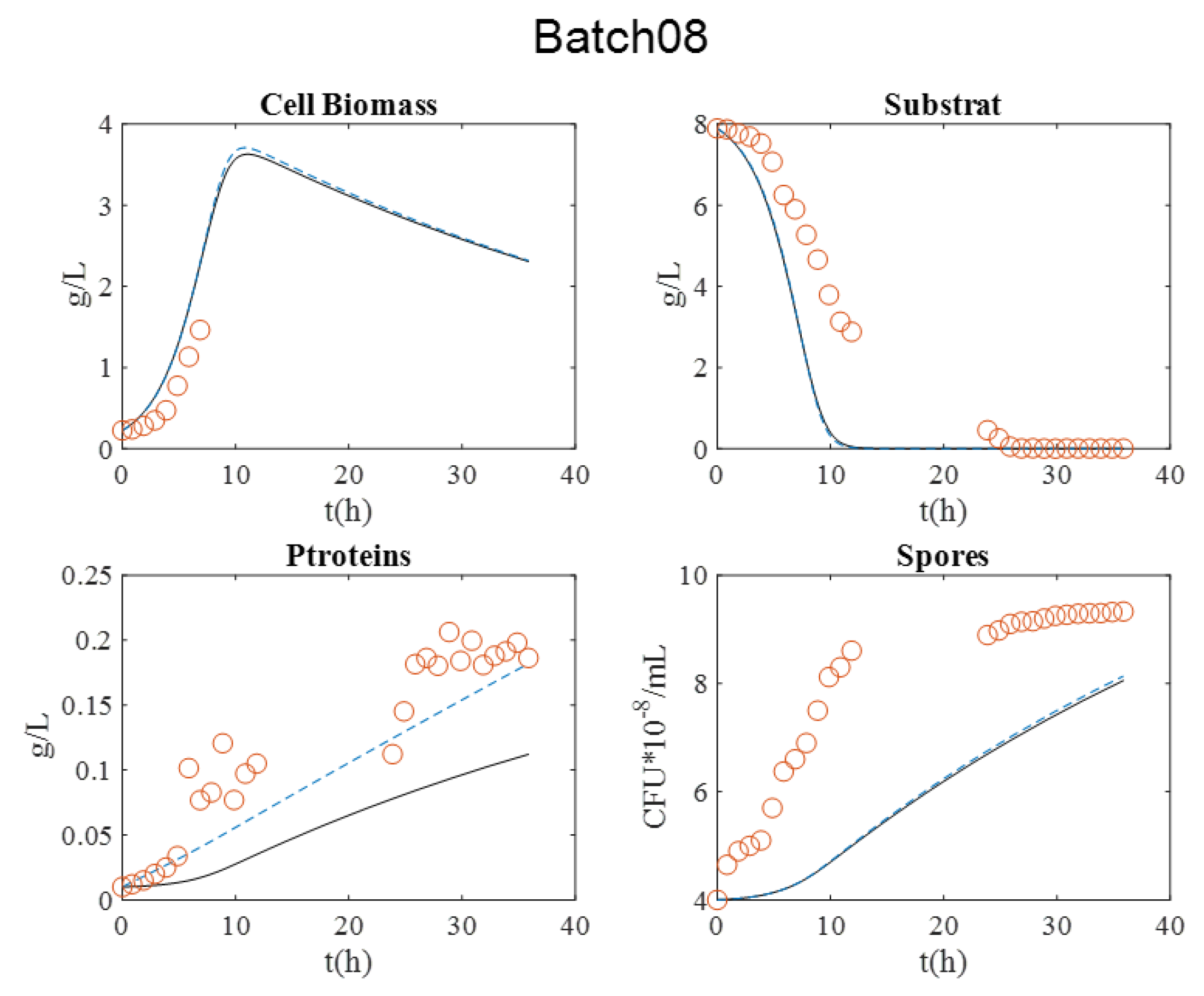
3.4.3. LIP Strain
4. Conclusions
Author Contributions
Funding
Institutional Review Board Statement
Informed Consent Statement
Conflicts of Interest
References
- Schnepf, E.; Crickmore, N.; Van Rie, J.; Lereclus, D.; Baum, J.; Feitelson, J.; Zeigler, D.R.; Dean, D.H. Bacillus thuringiensis and Its Pesticidal Crystal Proteins. Microbiol. Mol. Biol. Rev. 1998, 62, 775–806. [Google Scholar] [CrossRef] [PubMed] [Green Version]
- Iriarte, J.; Porcar, M.; Lecadet, M.-M.; Caballero, P. Isolation and Characterization of Bacillus thuringiensis Strains from Aquatic Environments in Spain. Curr. Microbiol. 2000, 40, 402–408. [Google Scholar] [CrossRef] [PubMed]
- Rowe, G.E.; Margaritis, A. Bioprocess design and economic analysis for the commercial production of environmentally friendly bioinsecticides from Bacillus thuringiensis HD-1kurstaki. Biotechnol. Bioeng. 2004, 86, 377–388. [Google Scholar] [CrossRef] [PubMed]
- El Khoury, M.; Azzouz, H.; Chavanieu, A.; Abdelmalak, N.; Chopineau, J.; Awad, M.K. Isolation and characterization of a new Bacillus thuringiensis strain Lip harboring a new cry1Aa gene highly toxic to Ephestia kuehniella (Lepidoptera: Pyralidae) larvae. Arch. Microbiol. 2014, 196, 435–444. [Google Scholar] [CrossRef] [PubMed]
- Navarro-Mtz, A.K.; Pérez-Guevara, F. Construction of a biodynamic model for Cry protein production studies. AMB Express 2014, 4, 79. [Google Scholar] [CrossRef] [PubMed] [Green Version]
- Holmberg, A.; Sievanen, R. Fermentation of Bacillus thuringiensis for Exotoxin Production: Process Analysis Study. Biotechnol. Bioeng. 1980, 22, 1707–1724. [Google Scholar] [CrossRef]
- Rivera, D.; Margaritis, A.; de Lasa, H. A sporulation kinetic model for batch growth of B. thuringiensis. Can. J. Chem. Eng. 1999, 77, 903–910. [Google Scholar] [CrossRef]
- Popovic, M.K.; Liu, W.-M.; Iannotti, E.L.; Bajpai, R.K. A Mathematical Model for Vegetative Growth of Bacillus thuringiensis. Eng. Life Sci. 2001, 1, 85–90. [Google Scholar] [CrossRef]
- Saadaoui, I.; Rouis, S.; Jaoua, S. A new Tunisian strain of Bacillus thuringiensis kurstaki having high insecticidal activity and δ-endotoxin yield. Arch. Microbiol. 2009, 191, 341–348. [Google Scholar] [CrossRef] [PubMed]
- Carozzi, N.B.; Kramer, V.C.; Warren, G.W.; Evola, S.; Koziel, M.G. Prediction of insecticidal activity of Bacillus thuringiensis strains by polymerase chain reaction product profiles. Appl. Environ. Microbiol. 1991, 57, 3057–3061. [Google Scholar] [CrossRef] [PubMed] [Green Version]
- Sarrafzadeh, M.H.; Guiraud, J.P.; Lagneau, C.; Gaven, B.; Carron, A.; Navarro, J.-M. Growth, Sporulation, δ-Endotoxins Synthesis, and Toxicity During Culture of Bacillus thuringiensis H14. Curr. Microbiol. 2005, 51, 75–81. [Google Scholar] [CrossRef] [PubMed]
- Bradford, O.F. Adaptation of the Bradford protein assay to membrane-bound proteins by solubilizing in glucopyranoside detergents. Anal. Biochem. 1987, 162, 11–17. [Google Scholar]
- Robles-Rodriguez, C.; Bideaux, C.; Gaucel, S.; Laroche, B.; Gorret, N.; Aceves-Lara, C. Reduction of metabolic models by polygons optimization method applied to Bioethanol production with co-substrates. IFAC Proc. Vol. 2014, 47, 6198–6203. [Google Scholar] [CrossRef]
- Burnham, K.P.; Anderson, D.R. Multimodel Inference: Understanding AIC and BIC in Model Selection. Sociol. Methods Res. 2004, 33, 261–304. [Google Scholar] [CrossRef]
- Robles-Rodriguez, C.E.; Bideaux, C.; Roux, G.; Molina-Jouve, C.; Aceves-Lara, C.A. Soft-Sensors for Lipid Fermentation Variables Based on PSO Support Vector Machine (PSO-SVM). In Proceedings of the 13th International Conference on Distributed Computing and Artificial Intelligence, Sevilla, Spain, 1–3 June 2016; pp. 175–183. [Google Scholar]
- Atehortúa, P.; Álvarez, H.; Orduz, S. Modeling of growth and sporulation of Bacillus thuringiensis in an intermittent fed batch culture with total cell retention. Bioprocess Biosyst. Eng. 2007, 30, 447–456. [Google Scholar] [CrossRef] [PubMed]


| Sol | Components | Semisynthetic (SSM) | LB |
|---|---|---|---|
| Peptone | - | 10 | |
| NaCl | - | 5 | |
| 1 | Yeast Extract | 0.5 | 5 |
| Casein acid hydrolysate | 4.5 | - | |
| (NH4)2SO4 | 6 | - | |
| K2HPO4 | 1.4 | - | |
| KH2PO4 | 1.4 | - | |
| 2 | Glucose | 5 | - |
| 3 | MgSO4, 7H2O | 0.61 | - |
| 4 | CaCl2, 2H2O | 0.332 | - |
| 5 | MnSO4, H2O | 0.006 | - |
| Strain | Batch |
|---|---|
| Btk. HD1 | B03, B04, B07 |
| Btk. BLB1 | B01, B02, B05, B06 |
| Btk. LIP | B08, B09, B10 |
| Parameter | BLB1 | |
|---|---|---|
| Model 1 | Model 2 | |
| µ max (h−1) | 1.1490 | 1.0720 |
| Kc | 4.7450 | 4.1250 |
| Kd (h−1) | 0.0437 | 0.0439 |
| Y1 gBiomass·gGlucose−1 | 0.7136 | 0.7141 |
| Y2 (gPro/gGlucose*h) | 0.0067 | 0.0067 |
| Y3 (CFU*10−5/gGlucose*h) | 0.0537 | 0.0524 |
| Alpha (g/L*h) | - | 0.0001 |
| Beta (CFU*10−5/L*h) | - | 0.0001 |
| Model | Criterion | Biomass | Glucose | Proteins | Spores | |
|---|---|---|---|---|---|---|
| Batch01 | 1 | R2 | 0.6902 | 0.9863 | 0.7088 | 0.1350 |
| RMSE | 0.4539 | 0.2445 | 0.2138 | 10.2994 | ||
| AICc | 29.5540 | 17.1797 | 14.4991 | 91.9945 | ||
| 2 | R2 | 0.6935 | 0.9835 | 0.7088 | 0.1357 | |
| RMSE | 0.4552 | 0.2711 | 0.2125 | 10.3321 | ||
| AICc | 149.6104 | 139.2478 | 134.3794 | 212.0580 | ||
| Batch06 | 1 | R2 | 0.5663 | 0.9976 | 0.7329 | 0.5756 |
| RMSE | 1.1693 | 0.1154 | 0.1633 | 2.2508 | ||
| AICc | 41.2816 | –9.6689 | –2.0279 | 55.6878 | ||
| 2 | R2 | 0.5686 | 0.9981 | 0.7337 | 0.5762 | |
| RMSE | 1.1699 | 0.0996 | 0.1638 | 2.2597 | ||
| AICc | 96.2913 | 42.1035 | 53.0457 | 110.7744 |
| Parameter | HD1 | |
|---|---|---|
| Model 1 | Model 2 | |
| µ max (h−1) | 0.5985 | 0.4024 |
| Kc | 1.4700 | 0.5140 |
| Kd (h−1) | 0.0458 | 0.0352 |
| Y1 gBiomass·gGlucose−1 | 0.9612 | 0.8333 |
| Y2 (gPro/gGlucose*h) | 0.0056 | 0.0050 |
| Y3 (CFU*10−5/gGlucose*h) | 0.0281 | 0.0001 |
| Alpha (g/L*h) | - | 0.0062 |
| Beta (CFU*10−5/L*h) | - | 0.1116 |
| Model | Criterion | Biomass | Glucose | Proteins | Spores | |
|---|---|---|---|---|---|---|
| Batch03 | 1 | R2 | 0.7086 | 0.9876 | 0.9763 | 0.9122 |
| RMSE | 0.7287 | 0.3705 | 0.1677 | 0.4863 | ||
| AICc | 39.0235 | 25.4968 | 9.6408 | 30.9351 | ||
| 2 | R2 | 0.7575 | 0.9803 | 0.9546 | 0.8486 | |
| RMSE | 0.6305 | 0.4203 | 0.0870 | 0.6881 | ||
| AICc | 156.1279 | 148.0185 | 116.5131 | 157.8768 | ||
| Batch04 | 1 | R2 | 0.7063 | 0.9992 | 0.7036 | 0.73007 |
| RMSE | 0.77276 | 0.0544 | 0.3128 | 2.7302 | ||
| AIC | 14.6311 | −22.5237 | 1.9751 | 32.3051 | ||
| 2 | R2 | 0.7666 | 1,0000 | 0.6469 | 0.7191 | |
| RMSE | 0.6203 | 0.0112 | 0.2140 | 1.5365 | ||
| AICc | –56.4420 | –112.6332 | –71.3404 | –43.7434 |
| Parameter | LIP | |
|---|---|---|
| Model 1 | Model 2 | |
| µ max (h−1) | 0.3966 | 0.3916 |
| Kc | 0.6899 | 0.5794 |
| Kd (h−1) | 0.0189 | 0.0193 |
| Y1 gBiomass·gGlucose−1 | 0.4866 | 0.4956 |
| Y2 (gPro/gGlucose*h) | 0.0005 | 0.0001 |
| Y3 (CFU*10−5/gGlucose*h) | 0.0213 | 0.0218 |
| Alpha (g/L*h) | - | 0.0042 |
| Beta (CFU*10−5/L*h) | - | 0.0002 |
| Model | Criterion | Biomass | Glucose | Proteins | Spores | |
|---|---|---|---|---|---|---|
| Batch09 | 1 | R2 | 0.6610 | 0.9387 | 0.8130 | 0.7747 |
| RMSE | 0.6795 | 0.7169 | 0.0472 | 0.9691 | ||
| AICc | 23.7638 | 25.0484 | –40.2561 | 32.2820 | ||
| 2 | R2 | 0.6653 | 0.9397 | 0.8377 | 0.7731 | |
| RMSE | 0.6992 | 0.7088 | 0.0289 | 0.9773 | ||
| AICc | 59.6479 | 59.9742 | –16.7948 | 67.6853 | ||
| Batch10 | 1 | R2 | 0.9528 | 1.0000 | 0.0002 | 0.6794 |
| RMSE | 0.6082 | 0.0083 | 0.1146 | 7.0190 | ||
| AICc | 35.4078 | –50.4395 | 2.0181 | 84.3253 | ||
| 2 | R2 | 0.9507 | 1.0000 | 0.0002 | 0.6796 | |
| RMSE | 0.5819 | 0.0039 | 0.0920 | 6.9800 | ||
| AICc | 154.5226 | 54.2584 | 117.6327 | 204.2139 |
| Model | Criterion | Biomass | Glucose | Proteins | Spores | |
|---|---|---|---|---|---|---|
| Batch02 | 1 | R2 | 0.1518 | 0.9195 | 0.3212 | 0.6722 |
| RMSE | 0.6181 | 0.2109 | 0.4249 | 17.9155 | ||
| AIC | 11.5082 | −3.5438 | 6.2621 | 58.6431 | ||
| 2 | R2 | 0.1484 | 0.9077 | 0.3225 | 0.6716 | |
| RMSE | 0.6275 | 0.2275 | 0.4229 | 17,9704 | ||
| AICc | −56.2800 | −70.4822 | −61.8033 | −9.3141 | ||
| Batch05 | 1 | R2 | 0.7510 | 0.9828 | 0.9047 | 0.9029 |
| RMSE | 0.5389 | 0.4323 | 0.1302 | 1.0764 | ||
| AICc | 32.9878 | 28.5794 | 4.5721 | 46.8259 | ||
| 2 | R2 | 0.7524 | 0.9814 | 0.9053 | 0.9029 | |
| RMSE | 0.5423 | 0.4433 | 0.1289 | 1.0345 | ||
| AICc | 153.1159 | 149.0829 | 124.3779 | 166.0305 |
| Model | Criterion | Biomass | Glucose | Proteins | Spores | |
|---|---|---|---|---|---|---|
| Batch07 | 1 | R2 | NC * | 0.9940 | 0.7991 | 0.4551 |
| RMSE | NC * | 0.3078 | 0.2263 | 30.1202 | ||
| AICc | NC * | −55.7705 | −71.7791 | 182.5655 | ||
| 2 | R2 | NC * | 0.9981 | 0.7720 | 0.3628 | |
| RMSE | NC * | 0.1337 | 0.3701 | 30.1186 | ||
| AICc | NC * | −91.0931 | −38.1445 | 190.6123 |
| Model | Criterion | Biomass | Glucose | Proteins | Spores | |
|---|---|---|---|---|---|---|
| Batch08 | 1 | R2 | NC * | 0.9883 | 0.8321 | 0.7054 |
| RMSE | NC * | 0.3716 | 0.0817 | 2.4370 | ||
| AICc | NC * | –45.9879 | –124.7646 | 51.8161 | ||
| 2 | R2 | NC * | 0.9878 | 0.8937 | 0.7042 | |
| RMSE | NC * | 0.3813 | 0.0351 | 2.4099 | ||
| AICc | NC * | –36.5917 | –160.6215 | 59.2837 |
Publisher’s Note: MDPI stays neutral with regard to jurisdictional claims in published maps and institutional affiliations. |
© 2021 by the authors. Licensee MDPI, Basel, Switzerland. This article is an open access article distributed under the terms and conditions of the Creative Commons Attribution (CC BY) license (https://creativecommons.org/licenses/by/4.0/).
Share and Cite
Monroy, T.S.; Abdelmalek, N.; Rouis, S.; Kallassy, M.; Saad, J.; Abboud, J.; Cescut, J.; Bensaid, N.; Fillaudeau, L.; Aceves-Lara, C.A. Dynamic Model for Biomass and Proteins Production by Three Bacillus Thuringiensis ssp Kurstaki Strains. Processes 2021, 9, 2147. https://doi.org/10.3390/pr9122147
Monroy TS, Abdelmalek N, Rouis S, Kallassy M, Saad J, Abboud J, Cescut J, Bensaid N, Fillaudeau L, Aceves-Lara CA. Dynamic Model for Biomass and Proteins Production by Three Bacillus Thuringiensis ssp Kurstaki Strains. Processes. 2021; 9(12):2147. https://doi.org/10.3390/pr9122147
Chicago/Turabian StyleMonroy, Tatiana Segura, Nouha Abdelmalek, Souad Rouis, Mireille Kallassy, Jihane Saad, Joanna Abboud, Julien Cescut, Nadia Bensaid, Luc Fillaudeau, and César Arturo Aceves-Lara. 2021. "Dynamic Model for Biomass and Proteins Production by Three Bacillus Thuringiensis ssp Kurstaki Strains" Processes 9, no. 12: 2147. https://doi.org/10.3390/pr9122147
APA StyleMonroy, T. S., Abdelmalek, N., Rouis, S., Kallassy, M., Saad, J., Abboud, J., Cescut, J., Bensaid, N., Fillaudeau, L., & Aceves-Lara, C. A. (2021). Dynamic Model for Biomass and Proteins Production by Three Bacillus Thuringiensis ssp Kurstaki Strains. Processes, 9(12), 2147. https://doi.org/10.3390/pr9122147