Abstract
A vision-based adaptive switching controller that uses optical flow information to avoid obstacles for micro unmanned aerial vehicles (MUAV) is proposed in this paper. To use the optical flow to indicate the distance between the MUAV and the environment, we propose an algorithm with multi-thread processing such that the optical flow information is obtained reliably and continuously in the entire camera field of view. The flying behavior of considered MUAV is regarded as a switching system when considering different flying modes during the mission of obstacle avoidance. By the required flight direction for obstacle avoidance specified by the detected optical flow, an adaptive control scheme is designed to track the required trajectory in switching modes. The simulation result shows the tracking performances of the adaptive control with the switching system. The experiment of the whole system is completed to verify the obstacle avoidance capability of our system.
1. Introduction
Recently, 3D robots have presented an increasingly prosperous market and rapid development. Many industries, such as automobiles, automation, surveillance, medical, etc., require robots to replace humans for various purposes. As for 3D robots, a lot of research of this field is specifically contributing to the aerial platforms. A micro unmanned aerial vehicle (MUAV) is an aircraft that can fly autonomously in response to dangerous situations, such as fire sites, chemical or nuclear disaster areas, and battlefields. Due to its low cost, small size and light weight, MUAV is light in weight and flexible, making it particularly suitable for performing tasks in indoor environments. In this article, we consider the navigation control of MUAV flying through stairs between building floors. We focus on designing a novel vision-based adaptive controller for MUAV obstacle avoidance.
To avoid obstacles during the flight missions, we need to estimate the distance through sonar, laser ranging, and infrared sensors to observe the environment around the MUAV. Nonetheless, the ranging or depth sensors are usually too big or have high power consumption such that they are hard to be mounted on an MUAV. Therefore, low-cost, small-size pinhole cameras are commonly used on MUAVs. Stereo cameras that are used on MUAVs [1,2,3] can also help to obtain the information for depth around the camera in the obstacle avoidance task. Considering the single camera, ground vehicles with a monocular camera installed at a fixed height can be used to estimate the distance to the off-road area [4]. When a single camera is installed on the MUAV, the optical flow is usually estimated to denote the distance between the camera and objects [5].
Optical flow has been widely applied in computer vision and robotics. The object tracking task may involve the feature point tracking of optical flow in the motion-based tracking method [6,7]. The optical flow can also be used to construct the environmental maps and obtain the motion of the camera itself [2,8]. Recently, some research has developed parallel computing algorithms on the graphics processing unit (GPU) [9] to quickly obtain optical flow; however, the cost of additional hardware and hard programming make its implementation difficult. In this work, we use a single camera to quickly and reliably extract the optical flow information in front of the MUAV, and then, the optical flow will help to generate the input commands designed by the controller, followed by processing them in parallel on the CPU computing platform. With the feedback signals extracted from the vision sensor and then utilized to control the motion for desired purpose, visual servoing is widely applied to different applications and robotic systems. In the visual servoing systems [10,11], the camera is mounted on a moving platform, such as the robot arm or ground/aerial vehicle, which is usually controlled to follow the target through the feedback of the target information in the images. In [12,13], the visual servoing system can assist the robot arm and agriculture robot to accomplish the tasks and achieve the satisfactory performance.
On the other hand, there are many works discussing the control of MUAV with various models and methods. The model and design of the considered MUAV is discussed in detail in [14,15], where some adaptive controller design approaches for different models are provided. In [16,17], the nonlinear control methods are proposed for MUAV with uncertain parameters. The state feedback adaptive controller for quadrotors with varying centers of gravity is also presented in [18]. In [19,20,21], a robust adaptive control is designed for MUAV with output feedback adaptive control. In [22], a visual adaptive control is proposed, in which they consider the vehicle dynamics and the image information to construct the controller. In [23], the visual servoing control is considered for an underactuated rotorcraft UAV to regulate its translational motion and heading orientation. Besides, variable structure control is also robust to the disturbances and is applied to the UAV system, as discussed in [24,25,26]. Most research considers the state feedback design, and it is assumed that the states can be obtained from the sensor. However, such an approach is expensive and may be impractical. In [27], the output feedback visual servoing control is employed to navigate the line following of UAV. Here, we treat the MUAV system as a black box with a switching transfer function and only employ the sensing information from a single camera. Moreover, the output feedback control of the switching system is designed with the observed image sequence, which is more practical for the implementation of the MUAV system.
In this work, we implement the obstacle avoidance task of the MUAV system on which the front camera installed, and we use the adaptive control with optical flow information. The feature point tracking by the Kanade–Lucas–Tomasi (KLT) [28,29] algorithm is first applied to generate the information of optical flow. However, the original KLT tracker has some limitations; for example, the tracked feature points should be in the texture image block. When tracking a common image block, the corresponding relationship of this point is only correct between several consecutive frames. Therefore, if we want to detect the optical flow for obstacle avoidance in the entire image space, the points will be drawn uniformly and quickly redrawn. Here, we applied the multi-threaded processing scheme to supplement the optical flow when redrawing. Since objects closer to the camera will generate greater optical flow, these image areas with large optical flow can be regarded as an infeasible flight space for obstacle avoidance. In addition, because it is undesirable to change the original flight direction of the MUAV mission during obstacle avoidance, the flight strategy of the MUAV is chosen to perform the forward and lateral movements without moving in the yaw direction. After selecting the desired collision avoidance flight direction, the forward and lateral actions will be activated in sequence to reduce the airflow disturbance from the MAV itself. Therefore, the dynamics of the MUAV are modeled as a switching system. The main contributions of this work are that we use the optical flow information by the vision sensor and design an adaptive controller with the output in which the transfer function is unknown and composed of switching parameters. Many existing results related to MUAV control use information about the entire state to control the system. Instead of using the state-space model, the plant of MUAV is considered as a black box with a switching system description under different operating modes.
The rest of this article is organized as follows. In Section 2, the multi-thread KLT tracker with uniform point distribution is proposed such that the optical flow information can be obtained in a more sufficient and reliable way. Section 3 describes the obstacle avoidance flight strategy with optical flow and the considered problems. Here, we also propose visual servoing and adaptive control of the switching system for MUAV. Section 4 provides some simulation and experimental results. Section 5 gives the conclusion.
2. Optical Flow Estimation for Detecting Obstacle
Since only a camera is mounted on the MUAV to capture the front view, the feasible flight path must be decided from the observed image frames. An MAV can estimate the relative distance between itself and an object by moving in the scene, which is based on the concept of visual odometry (VO) [30] or structure of motion (SFM) [31]. The image scene consistency between consecutive frames employs the KLT feature point tracker [29]. The relative distance between the MUAV and the surrounding object can be denoted by the feature point displacement, which is also called optical flow. The traditional KLT tracker is easy to be misled by disturbers and may not estimate abundant optical flow in the whole image frame. Therefore, we improve the KLT tracker to be a multi-threaded process with uniform point distribution such that the optical flow in whole image frame can be quickly and consistently obtained.
2.1. The Construction of Uniform Point Distribution
The traditional KLT tracker only adopts the significant feature points, which could be reliably identified across image frames, such as Harris corner detection and scale invariant feature transform (SIFT). As illustrated in Figure 1a, the selected corner points can be recognized robustly for a long time by using the KLT tracker with pyramid computation architecture [32]. However, the obtained optical flow is limited to the textured area. The image region with uniform appearance cannot detect the optical flow, where the relative distance information will be lost. The available flight space of MUAV would not be clearly identified for the visual servoing of obstacle avoidance.
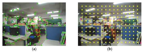
Figure 1.
Comparison of point distribution for evaluating optical flow. (a) Harris corner points selection; (b) uniformly distribute points.
Therefore, the optical flow information that will be utilized for the obstacle avoidance must fill the entire front camera’s field of view. Instead of selecting the corner points, we uniformly draw the points, which are then tracked by the KLT method in the image, as shown in Figure 1b. The points are also drawn on the uniform appearance image region. However, as demonstrated in Figure 2, the points drawn on the uniform appearance region as Figure 2a are easily misled by the similar neighbors after KLT tracking over than ten frames. These wrong tracked points also result in the incorrect optical flow as shown in Figure 2b. Since the life cycle of insignificant point tracking is very short, in order to improve their reliability, the uniformly drawn points must be quickly redrawn after KLT tracking several frames. As demonstrated in Figure 3, most of the points uniformly drawn in Frame #1 are successfully tracked in the following two frames (#2 and #3), even in the uniform appearance image region. In addition, during the MUAV flight, the identified points may disappear due to moving out of the camera’s field of view or being occluded by other objects. As shown in in Frame #1 and #4, considering the fast redrawing frequency can also quickly compensate the optical flow information when the points are missing or tracking is lost.
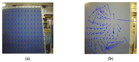
Figure 2.
The tracking result of the KLT point on the blue board under the camera shake. (a) Uniformly distribute points in the beginning; (b) tracking results after fifteen frames.
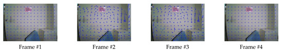
Figure 3.
The blue arrows denote the estimated optical flow vectors when the camera moves to the wall. We quickly redraw points uniformly every three frames.
2.2. Multi-Thread Processing
The KLT tracker with high frequency of point uniformly redrawing brings the disadvantage that identified optical flow is all erased when the tracked points are redrawn. At that time, the MUAV has no information to navigate the MUAV for obstacle avoidance. Here, a multi-thread processing for continuously obtaining the optical flow information is proposed to solve this problem. As shown in Figure 4, multiple threads are set to execute the pyramid Lucas–Kanade algorithm at the same time, and the point redrawing time of each thread is different. Assuming that there are KLT threads, each thread redraws the points at every frames, which cannot be too long, as described above. If the first thread redraws the point at frame , the following thread will redraw the points at frame . The image displacement is more pronounced on threads with longer tracking points. Therefore, the considered optical flow uses the thread farthest from its point redrawing moment and is defined as
where is current time, and is the recent point redrawing instant of the thread. The tracking process of multiple KLTs running one image frame in serial programming will be very slow, so point tracking is easy to fail. Fortunately, with the multi-core architecture of CPU, we can assign each tracking thread to a core of CPU. Then, as illustrated in Figure 5a, the optical flow in the entire camera field of view can be reliably and continuously detected with real-time performance.
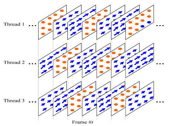
Figure 4.
Multi-thread KLT flow on the image sequence. In this example, there are three threads, and each thread will uniformly redraw the points in every three frames (frames with orange dots). The blue arrows illustrate the estimated optical flow vectors of the drawn orange points.
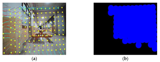
Figure 5.
Using the length of optical flow to determine feasible flight space. (a) Optical flow (the yellow dots denote the tracked points, and the red and cyan trajectories are the optical flow vectors); (b) feasible flight space (the blue region).
Since the object closer to the camera will cause the larger image displacement across image frames, the optical flow estimated through the multi-thread process can be used to avoid obstacles in front of the MUAV. By calibrating the camera on the MUAV, the maximum allowable length of the optical flow, which denotes the minimum safe distance between a stationary object and the fastest-moving MUAV, can be measured in the beginning. As presented in Figure 5, the optical flow with length shorter than the maximum allowable length will result in the feasible flight space. The image centroid of the estimated feasible flight space can then be employed to navigate the flight trajectory of the MUAV.
3. Visual Servoing with Adaptive Control of Switched Systems
We discuss the visual servoing problem of MUAV that uses adaptive control to implement obstacle avoidance commands. In the first stage, the MUAV is modeled as a third-order system with different parameters, when operating in different modes, such as rotation or translation. Then, the controlled object is regarded as a switching system, and an adaptive control design is proposed for the switching linear system with unknown parameters in the MUAV model.
3.1. System Description and Problem Formulation
Consider a quad-rotor MUAV equipped with a camera to capture the front view of the MUAV. Assume that the optical center of the camera is the same as the centroid of the MUAV, and the camera coordinates are the same as the coordinates of the MUAV body, as shown in Figure 6. To maintain the original flight direction of the MUAV mission, its heading direction will not change during the obstacle avoidance. The control input adopts the up and down speed along the axis, the lateral speed along the axis, and the forward speed along the axis. The horizontal image position is used to determine the horizontal movement of the MUAV, and the vertical image position is used to draw the vertical movement. Here, the speed is only used to keep the height fixed, and no information of is needed. The forward and lateral speeds are designed to avoid obstacles. As shown in Figure 7, given image observation and camera parameter , tangent function of the flight direction required to avoid obstacles in the transverse plane is expressed as
in which and are the needed forward and lateral displacement at current time instant , respectively. In practical implementation, values of and during one sampling period will be bounded in a feasible range, and the forward displacement is first selected with the inverse proportional to the maximum length of detected optical flow or proportional to the minimum estimated distance of the surroundings [6] at every frame. Notice that the lateral displacement is equal to zero when the desired flying direction is exactly in front of the MUAV, i.e., .
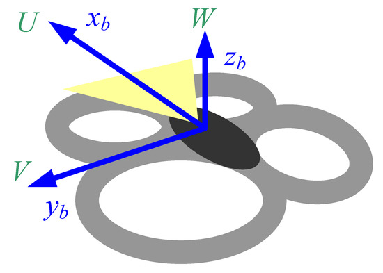
Figure 6.
MUAV body coordinate system. (Yellow region: camera field of view).
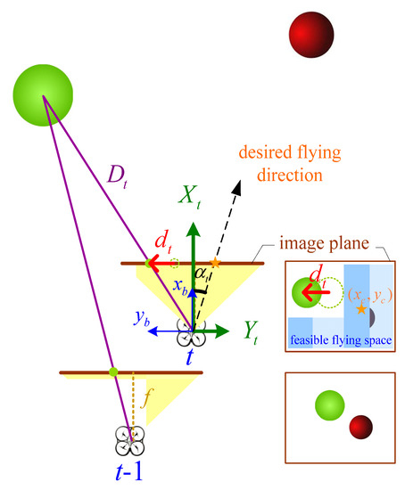
Figure 7.
The MUAV flies toward the desired flying direction on image plane.
By the operating behavior and dynamics of MUAV system, we make the assumption that the dynamical model of MUAV is approximated by a third-order transfer function whose relative degree is 1, which is from the observation of the experimental setting with the step reference. Through system identification, the modes of the quadrotor can be modeled as the following different transfer functions. The forward mode TF1 is , which is the forward translation in speed . The transverse mode TF2 is , which is the translation in speed .
From the observation point of view, the MUAV is easy to be disturbed by the airflow in the indoor environment when executing the commands of the two modes at each instant. Therefore, it is desirable to activate the flight mode in turn at each moment. The entire structure of the closed-loop system is given in Figure 8. The considered system decouples the axis and the axis separately, and they correspond to the forward mode and the lateral mode, respectively. For the axis, suppose the system is in forward mode, then its dynamics will be TF1. If the system changes to the lateral mode, its model will be TF2. The same is true for the axis. It is worth mentioning that for the axis, the reference is zero in the lateral mode (TF2) and remains unchanged in the forward mode (TF1). In contrast, when considering the axis, the reference is zero in the forward mode (TF1) and remains unchanged in the lateral mode (TF2). In Figure 8, blocks and are the controllers with respect to axis and the axis. Due to the inaccuracy of the approximate model and the uncertainty, the MUAV system parameters are regarded as unknown, and a robust adaptive control design is proposed to control the switching plants with unknown parameters in each mode.
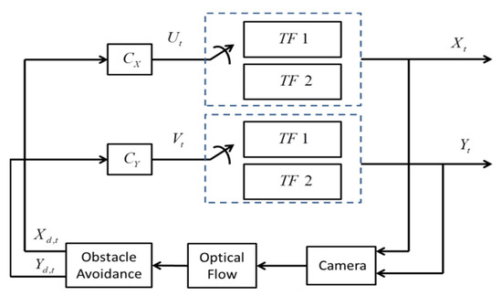
Figure 8.
The structure of the switched system for MUAV visual servoing.
3.2. Adaptive Control for Switched System
As shown in Figure 8, we design the adaptive control for the MUAV system with different modes and regard it as a switching system. For simplicity, we will discuss the general form in (3) below, which can be applied to the situation considered in Figure 8. For switching system with the transfer functions
where is the switching signal, and
The output y in (3) may be represented by or , and the input u is or , respectively.
The are assumed to be strictly proper with unknown parameters. Our control goal is to design the adaptive control so that the output signal will track the desired signal . The signals and are the references for the axis and the axis, respectively. In order to design an adaptive controller for the switching system (3), we pose the following conditions which are common in adaptive control system:
- (A1)
- The relative degree of the transfer function is and the order is n.
- (A2)
- The first time derivatives of the signal are all known and bounded.
- (A3)
- The transfer functions are completely controllable and observable.
- (A4)
- The signs of are known and are the same for all .
- (A5)
- The unknown parameters are bounded in a compact set which is known.
In order to design the adaptive control of the switching system, we adopted the tuning function method introduced in [29]. An output feedback backstepping control based on a variable structure is designed to make the tracking error under any switching signal converge to zero. In the first step, we use the adaptive observer with K filter [33] to estimate the states. System (3) is rewritten as
Here,
and
Then, we define as the ith coordinate vector, in which all components are zero, but the ith component is 1. Let such that is Hurwitz, by which there will exist a positive definite matrix that satisfies
The K-filters design observer is:
Define the virtual state estimator to be
and let the error of estimation as . The value of will decrease to zero exponentially with . According to the form of , we denote , where are column vectors that are found from a filter of input u, and are obtained from the filter of output . The K-filters are implemented as follows
Based on the above discussion, we design a backstepping adaptive controller with the K-filters and the tuning function approach. As the relative degree is one, according to (4),
From (5) and (8), we can represent as
The sub-index 2 stands for the second component in the column vector and stands for the second row of . Thus,
Denote the output error as , then
Thus, the control is chosen as
where is the estimate of , and
where . To handle the parameters with switching, our control parameters are designed by the variable-structure-based adaptive laws
The adaptive control is proposed by the Lyapunov theorem, where the Lyapunov function candidate is
Thus,
Note that in the first inequality in (16), the following relation is used
Here, , and we use (14) and the relation
for our derivations. By the analysis, we obtain that and will converge to zero exponentially and, thus, guarantee that is bounded. We then show that the remaining states are bounded by the filters. By (13) and the boundedness of , the control is bounded. Since is stable, and is bounded, this implies the boundedness of . Furthermore, is bounded due to the stability of and boundedness of y. Follow the above discussion and with (10), the boundedness of is guaranteed. Thus, the boundedness of is obtained by the boundedness of . From the analysis, the whole system is stable, and the output signal will asymptotically track the reference signal.
Remark 1. In the general relative degree case of tuning function adaptive control design, an assumption on minimum phase is required [33]. Here, this assumption is unnecessary, since we only consider the case where the relative degree is 1.
4. Simulation Analysis and Experimental Results
4.1. Simulation Analysis
The following simulation is first performed to verify the results of Section 3. In order to demonstrate the robustness of proposed controller in switching modes, we assume that the reference , the trajectory in axis, and mode of the plane are changing every second, which are given in Figure 9. Similar to results in the literature such as [34], the transfer function we consider is as follows, which is obtained through experiments.
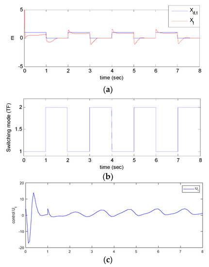
Figure 9.
Trajectory tracking performance for axis. (a) Comparison between the output trajectory and reference trajectory; (b) switching mode; (c) control input.
We can see that no matter how the controlled object mode is switched, the output will gradually track the reference. Nevertheless, some transience caused by the switching effect of the reference trajectory exist. The transient behavior here is not caused by switching parameters, but by the reference. The switching effects are suppressed by the robust variable structure adaptive controller, and thus, in the simulations, there is no obvious switching effect on the state trajectory. It is similar to the response . In addition, in (11), we utilize the condition for the case under consideration because of the measure zero property of the nondifferentiable points.
4.2. Experimental Results with Visual Servoing
As discussed in Section 2, our visual detection of obstacles uses the mentioned optical flow estimation. The multi-threaded process for detecting the optical flow is realized on four threads of a PC with quad-core 3.3GHz CPU, and each thread redraws the points turn by turn in every four frames. We use Drone 2.0 of Parrot AR as the MUAV to test our visual servoing method. The real-time performance, i.e., 30 frames per second, can be achieved for the computation process of visual detection and visual servoing.
In Figure 10, the blue circle represents the desired flight direction in the image frame, and the MUAV flight snapshot received from the third view is shown in Figure 11. The original flight direction to the MUAV is chosen to pass through the corridor indoor. In the flight procedure, the MUAV first detects the brown box in the corridor. The desired flight direction is specified by the center of mass of feasible flight space for avoiding the obstacles. The feasible flight space is adjusted to the left, and the MUAV takes turns to activate the forward mode and the lateral mode through the box. However, this avoidance caused the MUAV to hit the wall at Frame #562. As previously mentioned, the wall caused a larger optical flow as the MUAV moves forward; the flight direction then changed to the right at Frame #585. The MUAV will also avoid the desk after Frame #602. With the vision-based obstacle avoidance method and the adaptive control of switching modes, the MUAV can avoid the obstacles and maintain the moving direction such that it can successfully traverse the corridor.
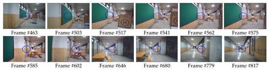
Figure 10.
Obstacle avoidance of MUAV. The image sequence is recorded from the camera on MUAV. The blue circle represents the desired flight direction in the image frame.
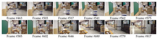
Figure 11.
Obstacle avoidance of the MUAV corresponding to Figure 10. The images are recorded from a third camera.
Moreover, as shown in Figure 12, we utilize the proposed visual servoing methodology to implement the moving obstacle avoidance task of MUAV. The blue circle denotes the desired flying direction in the image domain. We can see that from Frame #1 to Frame #170, the original desired flying direction is going toward the center of the corridor. The moving obstacle (human body) is observed by the multi-thread optical flow estimation in Frame #172, and the desired flying direction successfully lead the MUAV to pass the obstacle from Frame #177 to Frame #189. Afterwards, from Frame #199 to Frame #238, the MUAV can go back and continue the original task of heading toward the corridor.
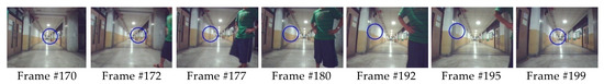
Figure 12.
Moving obstacle avoidance of the MUAV. The image sequence is recorded from the camera on the MUAV.
5. Conclusions
In this research, we propose a vision-based obstacle avoidance system with respect to the MUAV flight control, including visual flight control and visual obstacle detection. In order to determine the infeasible flight space, obstacle detection considers the optical flow information. In addition, for having sufficient optical flow with KLT, we need the feature points to be spread evenly in entire image frames. We develop the multi-threaded process by feature point tracking with KLT and take turns to quickly redraw the points. Thus, reliable optical flow is extracted. According to the information from optical flow, we select the direction of desired flight trajectory, and the MUAV moves forward and laterally to avoid obstacles. This paper proposes a visual servo controller with adaptive law for MUAV. As for the obstacle avoidance tasks, MUAV is modeled by the switching system, and we design the adaptive control to fulfill our control goals. Many existing results consider state feedback control and use a lot of sensors; here, we only consider one single camera to be the sensor for the proposed control system.
In future works, a visual servoing with a nonlinear switched model will be considered for the MUAV system. More flying modes of the switched system will be modeled for the MUAV behaviors in the indoor environment, such as the wondering, corridor or staircase crossing, object tracking, etc. The visual information of various environments will also be extracted as the basis of visual servoing in the corresponding scenarios.
Author Contributions
Data curation, K.-T.T.; formal analysis, M.-L.C. and S.-H.T.; investigation, S.-H.T.; methodology, M.-L.C. and C.-M.H.; software, S.-H.T. and K.-T.T.; supervision, C.-M.H.; writing—original draft, M.-L.C. and C.-M.H. All authors have read and agreed to the published version of the manuscript.
Funding
This research was funded by Ministry of Science and Technology, Taiwan, grant number MOST 109-2221-E-027-111, MOST 109-2221-E-029-026, MOST 110-2221-E-029-028, and MOST-110-2221-E-110-067.
Acknowledgments
The authors would like to express their sincere gratitude to the anonymous reviewers who gave us many constructive comments and suggestions. This work was supported in part by the Ministry of Science and Technology, Taiwan, under the grants: MOST 109-2221-E-027-111, MOST 109-2221-E-029-026, MOST 110-2221-E-029-028, and MOST-110-2221-E-110-067.
Conflicts of Interest
The authors declare no conflict of interest.
References
- Yu, H.; Beard, R.W.; Byrne, J. Vision-based local multi-resolution mapping and path planning for miniature air vehicles. In Proceedings of the 2009 American Control Conference, St. Louis, MO, USA, 10–12 June 2009; pp. 5247–5252. [Google Scholar]
- Fraundorfer, F.; Heng, L.; Honegger, D.; Lee, G.H.; Tanskanen, P.; Pollefeys, M. Vision-based autonomous mapping and exploration using a quadrotor MAV. In Proceedings of the 2012 IEEE/RSJ International Conference on Intelligent Robots and Systems, Vilamoura-Algarve, Portugal, 7–12 October 2012; pp. 4557–4564. [Google Scholar]
- Baraian, A.; Nedevschi, S. Improved 3D Perception based on Color Monocular Camera for MAV exploiting Image Semantic Segmentation. In Proceedings of the 2019 IEEE 15th International Conference on Intelligent Computer Communication and Processing (ICCP), Cluj-Napoca, Romania, 5–7 September 2019; pp. 295–301. [Google Scholar]
- Hsu, C.M.; Lian, F.L.; Huang, C.M.; Chang, Y.S. Detecting drivable space in traffic scene understanding. In Proceedings of the 2012 International Conference on System Science and Engineering, Dalian, China, 30 June–2 July 2012; pp. 79–84. [Google Scholar]
- Zingg, S.; Scaramuzza, D.; Weiss, S.; Siegwart, R. MAV navigation through indoor corridors using optical flow. In Proceedings of the IEEE International Conference on Robotics and Automation (ICRA), Anchorage, AK, USA, 3–7 May 2010; pp. 3361–3368. [Google Scholar]
- Brox, T.; Rosenhahn, B.; Gall, J.; Cremers, D. Combined region and motion-based 3D tracking of rigid and articulated objects. IEEE Trans. Pattern Anal. Mach. Intell. 2010, 32, 402–415. [Google Scholar] [CrossRef]
- Chmielewski, P.; Sibilski, K. Ground Speed Optical Estimator for Miniature UAV. Sensors 2021, 21, 2754. [Google Scholar] [CrossRef]
- Irfan, M.; Dalai, S.; Kishore, K.; Singh, S.; Akbar, S.A. Vision-based Guidance and Navigation for Autonomous MAV in Indoor Environment. In Proceedings of the 2020 11th International Conference on Computing, Communication and Networking Technologies (ICCCNT), Kharagpur, India, 1–3 July 2020; pp. 1–5. [Google Scholar]
- Pauwels, K.; Tomasi, M.; Alonso, J.D.; Ros, E.; van Hulle, M.M. A comparison of FPGA and GPU for real-time phase-based optical flow, stereo, and local image features. IEEE Trans. Comput. 2012, 61, 999–1012. [Google Scholar] [CrossRef]
- Chaumette, F.; Hutchinson, S. Visual servo control. I. Basic approaches. IEEE Robot. Autom. Mag. 2006, 13, 82–90. [Google Scholar] [CrossRef]
- Tsai, D.; Dansereau, D.G.; Peynot, T.; Corke, P. Image-Based Visual Servoing With Light Field Cameras. IEEE Robot. Autom. Lett. 2017, 2, 912–919. [Google Scholar] [CrossRef] [Green Version]
- Popescu, D.; Mihai, V.; Cojocaru, J.-I.-R.; Drăgana, C.; Ichim, L. Visual Servoing System for Local Robot Control in a Flexible Assembly Line. In Proceedings of the 2020 28th Mediterranean Conference on Control and Automation (MED), Saint-Raphaël, France, 15–18 September 2020; pp. 927–932. [Google Scholar] [CrossRef]
- Keshmiri, M.; Xie, W.; Mohebbi, A. Augmented Image-Based Visual Servoing of a Manipulator Using Acceleration Command. IEEE Trans. Ind. Electron. 2014, 61, 5444–5452. [Google Scholar] [CrossRef]
- Schreier, M. Modeling and adaptive control of a Quadrotor. In Proceedings of the IEEE International Conference on Mechronics and Automation (ICRA), Chengdu, China, 5–8 August 2012; pp. 383–388. [Google Scholar]
- Outeiro, P.; Cardeira, C.; Oliveira, P. Multiple-model control architecture for a quadrotor with constant unknown mass and inertia. Mechatronics 2021, 73, 102455. [Google Scholar] [CrossRef]
- Diao, C.; Xian, B.; Gu, X.; Zhao, B.; Guo, J. Nonlinear Control for an underactuated quadrotor unmanned aerial vehicle with parametric uncertainties. In Proceedings of the 31st Chinese Control Conference, Hefei, China, 25–27 July 2012; pp. 998–1003. [Google Scholar]
- Zhou, X.; Dai, X.; Li, Y. Nonlinear Dynamics Decoupling Control for a Light and Small Inertially Stabilized Platform. In Proceedings of the 2021 6th IEEE International Conference on Advanced Robotics and Mechatronics (ICARM), Chongqing, China, 3–5 July 2021; pp. 663–666. [Google Scholar]
- Palunko, I.; Fierro, R. Adaptive control of a quadrotor with dynamic changes in the center of gravity. IFAC Proc. Vol. 2011, 44, 2626–2631. [Google Scholar] [CrossRef] [Green Version]
- Nicol, C.; Macnab, C.J.B.; Ramirez-Serrano, A. Robust adaptive control of a quadrotor helicopter. Mechatronics 2011, 21, 927–938. [Google Scholar] [CrossRef]
- Hamela, T.; Mahony, R. Image based visual servo control for a class of aerial robotic systems. Automatica 2007, 43, 1975–1983. [Google Scholar] [CrossRef] [Green Version]
- Dong, G.; Cao, L.; Yao, D.; Li, H.; Lu, R. Adaptive Attitude Control for Multi-MUAV Systems with Output Dead-Zone and Actuator Fault. IEEE/CAA J. Autom. Sin. 2021, 8, 1567–1575. [Google Scholar] [CrossRef]
- Lee, D.; Nataraj, C.; Burg, T.C.; Dawson, D.M. Adaptive tracking control of an underactuated aerial vehicle. In Proceedings of the Proceedings of the 2011 American Control Conference, San Francisco, CA, USA, 29 June–1 July 2011. [Google Scholar]
- Li, J.; Xie, H.; Low, K.H.; Yong, J.; Li, B. Image-Based Visual Servoing of Rotorcrafts to Planar Visual Targets of Arbitrary Orientation. IEEE Robot. Autom. Lett. 2021, 6, 7861–7868. [Google Scholar] [CrossRef]
- Ali, Z.A.; Pandey, S. Variable Structure-Model Reference Adaptive Control for Stabilization the Attitude of UAV. Int. J. Control. Autom. 2017, 10, 37–48. [Google Scholar] [CrossRef]
- Kashkul, M.; Saberi, F.F.; Kasiri, A. Variable structure control of quadrotor based on position input. In Proceedings of the 2021 7th International Conference on Control, Instrumentation and Automation (ICCIA), Tabriz, Iran, 23–24 February 2021; pp. 1–6. [Google Scholar]
- Derrouaoui, S.H.; Bouzid, Y.; Guiatni, M. Nonlinear Robust Control of a New Reconfigurable Unmanned Aerial Vehicle. Robotics 2021, 10, 76. [Google Scholar] [CrossRef]
- Rafique, M.A.; Lynch, A.F. Output-Feedback Image-Based Visual Servoing for Multirotor Unmanned Aerial Vehicle Line Following. IEEE Trans. Aerosp. Electron. Syst. 2020, 56, 3182–3196. [Google Scholar] [CrossRef]
- Shi, J.; Tomasi, C. Good features to track. In Proceedings of the IEEE Conference on Computer Vision and Pattern Recognition, Seattle, WA, USA, 21–23 June 1994; pp. 593–600. [Google Scholar]
- Joseph, H.; Rajan, B.K. Real Time Drowsiness Detection using Viola Jones & KLT. In Proceedings of the 2020 International Conference on Smart Electronics and Communication (ICOSEC), Trichy, India, 10–12 September 2020; pp. 583–588. [Google Scholar]
- Scaramuzza, D.; Fraundorfer, F. Visual odometry: Part I—The first 30 years and fundamentals. IEEE Robot. Autom. Mag. 2011, 18, 80–92. [Google Scholar] [CrossRef]
- Tomasi, C. Shape and motion from image streams under orthography: A factorization method. Int. J. Comput. Vis. 1992, 9, 137–154. [Google Scholar] [CrossRef]
- Bouguet, J.Y. Pyramidal Implementation of the Lucas Kanade Feature Tracker Description of the Algorithm; Intel Corporation Microprocessor Research Labs: Santa Clara, CA, USA, 2000. [Google Scholar]
- Krstic, M.; Kanellakopoulos, I.; Kokotovic, P. Nonlinear and Adaptive Control Design; John Wiley & Sons: Hoboken, NJ, USA, 1995. [Google Scholar]
- Ahmed, A.H.; Ouda, A.N.; Kamel, A.M.; Elhalwagy, Y.Z. Design and Analysis of Quadcopter Classical Controller. In Proceedings of the 16th International Conference on Aerospace Sciences & Aviation Technology, Cairo, Egypt, 26–28 May 2015. [Google Scholar]
Publisher’s Note: MDPI stays neutral with regard to jurisdictional claims in published maps and institutional affiliations. |
© 2021 by the authors. Licensee MDPI, Basel, Switzerland. This article is an open access article distributed under the terms and conditions of the Creative Commons Attribution (CC BY) license (https://creativecommons.org/licenses/by/4.0/).