Abstract
In closed-loop control systems, the model accuracy exerts large influences on the controllability, stability and quality of the whole process. Among all the faults that could affect the system performance, Model Plant Mismatch (MPM) is the one that not only directly threatens the system stability but also deteriorates the controller performance. Meanwhile, MPM has a major influence on the qualities of outputs about industrial products. In this work, a new detection method based on Granger Causality is proposed to detect and locate the MPM in multiple input multiple output systems. Causality can reflect the relations between the mismatch fault and its negative effects on model predictive control(MPC) systems. With the assistance of disturbance transfer function models, the causality method can further be used to locate the mismatch positions and get the correct channels of each kind of mismatches. The proposed method was examined and validated in the Wood-Berry process in contrast to the decussation location method under model predictive controller.
1. Introduction
Model Predictive Control (MPC) has been occupying a dominant position in advanced control technologies in the industrial production processes [1] due to its maturation in the controller selection, its ability to address complex constraints on closed-loop systems [2] and its preferable control effects and superior optimization results [3]. Therefore, MPC has received much attention and adoption as an advanced controller in some industrial processes [4]. However, the superiority in MPC versus other typical controllers such as Proportional-Integral-Differential(PID), is on account of its model-based structure and model-oriented optimization design [5]. Hence, the model accuracy imposes considerable influence on the control effects and output production qualities [6], and somehow makes the control stability untrue for engineering practice [7].
Thus far, fault diagnosis has attracted increasing interests in process control community in recent decades. Considering that most diagnosis technologies based on data driven methodology can reflect the control effects but provide little information on the variation of the controlled models, Model Predictive Control technology, whose control performance relies largely on the process models, gets less assistance from pure data methods. Model-based diagnosis methods, rely on a model that defines nominal behavior of a dynamic system to detect abnormal behaviors and isolate faults. On the other hand, data-driven diagnosis algorithms detect and isolate system faults by operating exclusively on system measurements and using very little knowledge about the system [8]. By comparison, the Control Performance Assessment (CPA) is associated with objective models to a certain extent, which embodies some statistical information or details of controlled models. Hence, CPA technologies were devised and designed as a series of controller monitoring and performance assessment methods for this reason.
Harris first introduced Minimum Variance Benchmark (MVB) into control systems as an assessment method to monitor the closed loops [9], creating a new world for assessing, analyzing, monitoring and managing the control performance. For evaluating the MVB index of Multiple Input and Multiple Output (MIMO) systems, the predicament is that a Nilpotent interactor matrix [10] is significant for the user but difficult to calculate for the computer. To avoid this inconvenience, Biao Huang ameliorated the Nilpotent algorithm and estimated a suboptimal benchmark with a reduction of priori knowledge of interactor matrix [11]. Jie Yu and S.Joe Qin invented left-right diagonal interactor rather than directly using Nilpotent interactor matrix as another auxiliary calculation method [12] for performance computation. However, the emergence and existence of Model Plant Mismatch (MPM) had had an impact on control performance evaluations [13] and even weakened the reliability of evaluating benchmark. In addition, time delay mismatch would affect the Minimum Variance Benchmark (MVB) and lead to the changes in both the system output variances and the Minimum Variance index [14].
Several literatures focus on quantifying the impact caused by model mismatch [15] or the design of suitable index to evaluate MPM problems [16]. Other scholars like Yucai Zhu used small sinusoidal test signals to detect the MPC model error [17] or identification of k-step-ahead prediction error in MPC to distinguish the difference between the nominal model and the real plant model [18]. However, the system identification technologies were purchased at too great a price for industrial production especially in closed loops [19]. Besides, most mismatch faults of chemical production affect a little fraction of stability but large proportion of performance. Therefore, it is much more appropriate for manufacturing industry to select MPM detection as the first option.
Among the great majority of detection methods, correlation analysis plays a most common technique role in model plant mismatch detection [20]. Abhijit S. Badwe used a partial correlation analysis method in MPC systems [21] to estimate the statistical characteristics while Siyun Wang estimated the MPC model mismatch by a means of auto-covariance analysis [22]. Gui Chen had the aid of mutual information to detect the model-plant mismatch of nonlinear multivariate systems. Viviane Botelho proposed a method of evaluating model quality based on the investigation of closed-loop data and the nominal output sensitivity function [23]. In practical terms, correlation estimation of variables could not be as accurate as expected. The natural relationship between any two types of different data and the complicated condition in the MIMO control systems after mismatch would increase the imprecision of correlation analysis techniques and reduce the probability of reliability of algorithms.
Some detection technologies are based on an orthogonal projection method [24] to analyze the extent and calculate the index of MPM problems [25]. However, detecting MPM would be a hot issue to address while locating the position of MPM would be another. Lijjuan Li defined the correlation analysis method between the input and the disturbance (CAID) index of assessing the MPM and presented the decussation thought, synthetically combining CAID method and model quality index (MQI) index together to get the specific location of mismatch [26]. During the process of estimation by orthogonal projection, the loss of data information is unavoidable to degrade a lot accuracy of the method. In the mean time, further variable correlation analysis depending on orthogonal projection will also be incorrect more or less, and mislead the judgment of location.
In this paper, we first introduce the Granger Causality Analysis (GCA) method of Model-Plant Mismatch detection in MIMO systems. The Granger Causality Analysis [27] expresses the direct relation between two variables with less dependence on statistical correlation and return back the cause and effect of MPM problems of MIMO systems with the help of closed-loop data. Considering that the Granger Causality Analysis might inevitably be influenced by the loop interconnection and the control strategies, we make further efforts to combine the noise models with Granger Causality Analysis (GCA) to locate the specific channel of MPM and the experiments on Wood-Berry distillation system are implemented after that.
2. Preliminaries
2.1. Model-Plant Mismatch in Closed-Loop Systems
To directly distinguish the difference of the nominal controlled model and the real process model, Internal Model Control (IMC) has been generally adopted in some control systems. An advantage which Internal Model Control structure is in possession of is that its feedback part promptly returning back the error of two models, the nominal model and the practical model , respectively. Hence, data from the control loops can conveniently help to cope with the MPM problems.
The block diagram of IMC structure of closed loop systems is depicted in Figure 1. The whole transfer function of system output is,
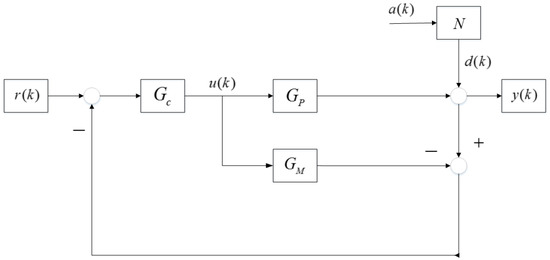
Figure 1.
Variables and model structure of Internal Model Control (IMC).
In the Equation (1) and the Figure 1, and represent the input setpoint value and the white noise disturbance, respectively. is the controller output sequence, namely manipulated variable, which is generated by the process controller . The sequence means the direct noise that is conducted into the control loops, which is produced by the white noise after disturbance transfer function N.
Direct Error Feedback Type of Internal Model Control changes the denominators of the whole transfer function of output and has an impact on control stability.
The controller acts directly on the process model in conventional control structure. Thus, the closed loop transfer function without IMC is presented as
It is obvious that the denominators in two transfer functions differ from each other by contrast Equation (1) with Equation (2).
The conventional controller is designed for the process model so that is in the service of the . If there is no mismatch, the result infers from the expression , which implies that the designed controller directly acts on the objective process. Once MPM occurred, controller would be applied to a new model in consideration of a primary fact that any devised controller had some robustness and could address a certain degree of model error.
However, in Equation (1), the controller should deal with not merely the two different models, but the deviation from controlled process, which means that the controller is designed for rather than or .
It is possible that can alter the model structure, parameters and even Pole-Zero points, which brings about a certain dilemma that the designed controller is insensible of its object models. The alteration of Pole-Zero points is able to worsen the stability of closed loop systems and elevate quite a few difficulties for the engineer to design a proper controller.
To overcome these shortcomings, putting the nominal model into the feedback section is advisable and the proof that this IMC structure influence nothing in comparison with Equation (2) is given later.
Theorem 1.
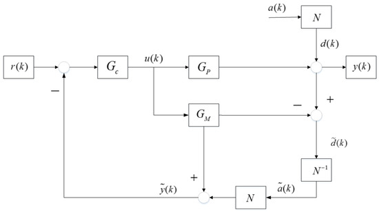
The structure of output transfer function in the schematic of Internal Model Control in Figure 2 is equivalent to that in Equation (2) and adds no burden to initial controller design.
Figure 2.
Schematic of noise-signal-estimation-mode in Internal Model Control Structure.
Proof of Theorem 1.
The relationship of all kinds of variables display as below,
The MPM problems are split into two circumstances. The first is that there is no mismatch in systems and the other is the occurrence of model plant mismatch conditions. when there is no state of MPM in the system, ,
Hence, the controller output sequence is expressed as
and the real control loop output result sequence is expressed as
Considering the fact that no mismatch occurs and , the Equation (7) is the same as the Equation (2).
When model mismatch happens, the relationships within variables are
At this moment, the controller law is
and the output data is
which is also the same sa before in Equation (2).
No matter whether there is model plant mismatch between these loops, the structure of control system transfer functions is invariant. Only model mismatch itself from the nominal model to the mismatched plant changes the parameters, which is rational and rational for daily operating systems.
The Theorem 1 is proved. □
2.2. Problem Description
The most common condition of closed loops in industrial production processes is steady-state but of unsatisfactory performance. As almost all the controlled process are linearized before implementation, it is a natural state that the real practical models must be somewhat different from the nominal ones that users had already designed the suitable controller for. Theoretically, the nominal linear model can accomplish its adaptation to the control system. However, manufacturing industries are always accompanied by many unexpected conditions, which result in the changes of industrial art or alteration of model parameters. Therefore, the occurrence of Model Plant Mismatch (MPM) can hardly be avoided.
A fundamental formula from the Equation (4) reflects that the variable consists of two portions, the model value difference with control law result and the pure disturbance signal that conducts into the closed loops.
The decussation location [26] drew supports from the statistical correlation between and . The existence of correlation within these two sequences is explicit but the conspicuousness of and in the computation of correlation can not get guaranteed. Besides, the sequence is estimated from loop data, which shows a big difference from the real noise signals.
The variable is generated by two sections, one of which presents the model discrepancy on MPM problems. The formula can be rewritten as
In this work, we bring and and Granger Causality Analysis together into MPM detection. One virtue of this formula is that it can represent whether there exists model plant mismatch in closed loop systems. Another merit is its reduction in the degree of difficulty to estimate and compute the signal sequence like or , which abates the data loss of orthogonal projection evaluation or system identification.
2.3. Introduction of Decussation Location
According to Figure 2, correlation analysis method between the input and the disturbance (CAID) focuses on the relationship between the controller effect and the estimated noise model . cannot be directly obtained from closed loops while an estimation method is required for further calculation. is the computation of CAID results.
The projection to the orthogonal complement of was introduced to finish this task. consists of two arranged variables.
and the orthogonal projection is,
The estimated sequences, and , are as below.
Model quality index (MQI) is a simple control performance assessment index for evaluating the systems. is the real noise model sequence while is an estimated one. Decussation location method contains two techniques, CAID and MQI, respectively. CAID is designed to locate the row channel mismatch while MQI is to detect the line channel.
3. Granger Causality Analysis
3.1. Causality
It was Granger who initially introduced causality and its practical implementation into economical data analysis [28]. Causality is one kind of data processing methods in the context of linear regression.
Assume that there are two stochastic processes and and both of them possess a feature that they can be modeled as an autoregressive linear process. Then the data can be written as two sections, an autoregressive sequence and remaining noise model .
The remaining model part is white noise with zero-mean and basic variance under normal conditions. “E()” is the symbol of data expectation, and “D()”, statistical variance.
As the sequence owns time feature, the data can be decomposed by its past information. Furthermore, auto-regression can reflect the relationship between the data and its past information to a certain degree. Since is generated by other reasons, auto-regression as well as noise model is not able to characterize all the causation at a time. If an engineer judges that the process could cause the change of , then a prediction will be made to testify the causality.
the mean value of white noise sequence is also zero and its variance changes to whose value becomes . If the predictability of is enhanced because of the existence of , there will exist causality from to .
The independence of and portends that is of no use for predicting the sequence so that and the index is zero, which shows there is no causality from to .
The index is composed of three portions, explicating the causality from to , causality from to and causality of as well as .
3.2. Causality for Detection the Mismatch
The best method to analyze the model plant mismatch is to address the issues by detecting or assessing the faults rather than identifying the coefficients in closed loops. Honestly, system identification is a recommendable detection means to monitor and diagnose the working condition, but this technique often encounters some realistic obstacles, such as numerous difficulties on dependability of detection and identification, data precision of results about model parameters, huge cost of implementation in closed loops, etc. More often, internal model control structure can embody both the nominal model and the practical one in just one closed loop and directly obtain model-plant differences. Lijuan Li [26] estimated the white noise and the input type disturbance and combined these with the controller output using statistical correlation. In view of that quite a few statistical approaches get interference from data and noise, estimated sequences do undergo such dilemmas. Granger causality analysis avoids this evaluation predicament, reduces the loss of data calculation and obtains the causality results of two or more sequences.
No matter whether there is model mismatch in the system, sequence contains the noise from beginning to end. In this section we use to represent the data sequence of variable , and to mean that of . is for and is for in the same way.
Every describes the corresponding coefficient of autoregressive sequences of . And indicates the model deviation quantity is hardly avoidable.
Theorem 2.
The existence of Causality
(i) represents actually, and it is also a type of white noise sequence.
(ii) Causality between and exists. can be used to predict .
Proof of Theorem 2.
The existence of Causality
For the models in Figure 2,
Transfer function of can be expanded to polynomials with implying the back shift operator.
Every discrete transfer function model can be expanded as above and their lengths are endless. Sequence number n tend to be infinite. When n is big enough, the left parameters remain to be zero in theory.
The model plays as conceptual deviation of the two models, which is nearly unable obtained or calculated in real industrial processes.
(i) If there is no mismatch occurring in the loop,
Expand to discrete polynomials,
Rearrange the Equation (27),
Compare the Equation (22) with Equation (28), the coefficient of is,
and the remaining noise model is
In the light of initial structure in Figure 2, the noise is white with zero mean. Hence, Proof (i) is done.
(ii) If model plant mismatch occurs in the process of chemical production,
Causality and correlation analysis methods are incapable of processing the noise, even system identification remains the noise part ultimately. Therefore, white noise is the only information left in the end.
Suppose that the sequence expansion of is
Then the prediction of will be,
Since the regression above is a new data processing, the coefficient should change from to and to . The left noise is variant of in the formula expression, too. The Equation (34) is a causality analysis from Equation (19), with sequence from a control loop to assess .
The white noise deems to be independent of other sequence and the relation of and is almost zero because of time delay in systems. The transfer function between and is
Generally refers to any transfer function from the beginning to the end . As the time delay acts on the control system, effect of this is equivalent to time lag for noise from to .
For white noise ,
is the variance of data from
The mathematical expectation of two data is zero.
means the left information about after Granger regression computation.
The variance of after regression, namely , consists of two sections. The first is information about noise and the second, . As the regression of could extract a little information about , the variance of always exists in the statistical characteristics in .
is the comprehensive coefficient mainly caused by .
It is obvious that the data of can help to influence the variance of . Therefore, causality of these two variables necessarily exists. Proof (ii) is finished. □
Theorem 3.
The alteration of MPM in parameters or model structure rather than mismatch position is independent of judgment on causality result.
So long as the model mismatch exists in the closed loop system, the increase or decrease of the practical model that is throughout different from the nominal model, and its type or other changes from the plant model, influence nothing of causality judgment.
Proof of Theorem 3.
When the real practical industrial model changes,
The time sequence of will raise to a new level.
A unified function here represents all kinds of model plant mismatches, and any change in the part of is included.
Even mismatch is varied from a former one, the regression variance information alters to a new one,
By promoting the level of regression for and that of auto-regression , the regression variance of decreases. It was not until the moment that the variance of dropped down to the minimum value that the causality analysis could be called as an accomplished algorithm.
The variance alteration mainly depends on and its coefficients . Considering that the variance of is greater than or equal to zero,
The Equation (51) indicates that the existence of model mismatch causes the causality among corresponding sequences. The Granger index shows the invariance of causality, namely the alteration of mismatch affecting the value of variances and Granger index but nothing on the causality judgment result. □
Theorem 4.
The increase of model orders results in the promotion of Granger index.
The judgment of causality is immune from model change in Theory 3. But the prediction of the variable is affected by data and model regression order. The raise of model orders leads to the monotone increase of Granger index.
(i) The increase of auto regressive model orders makes the variance of auto regression reduce to a lower bound. And the minimum variance is that of white noise with value .
(ii) The variance of gets its reduction due to the prediction of and its minimum value is the same as before.
(iii) The Granger index increases with the increase of model orders.
Proof of Theorem 4.
The raise of model orders results in monotone increasing of Granger index.
The summation in Equation (34) is composed of infinite sequences, which means . But in practice, all the regressions can not be implemented to infinite parts. In addition, when the number n is big enough, the left infinite sequences incline to zero. Thus, it is not necessary to calculate more dispensable data. Assume that the model orders selected are for and for , respectively.
As it is essential for regression analysis that the regression part should be deleted, The left part information is described as ,
The remaining sequences reflect the data that cannot be used or got further regressions.
When model order increases from to ,
In steady systems, the data contains the information of and mismatch. Hence, it can be written as,
Rewrite the formua as,
is the regression variance of symbol . As the auto-regression can only contain little information on mismatch transfer function and seldom include the controller output sequence , the variance is composed of two different parts. is generated from white noise of systems while variance of manipulated variable comes from MPC in practice.
The coefficients of is decomposed into three parts, , , . implies that when the regression length of is , a certain variance will be extracted from , and its weighting factor will be .
Seeing that regression from to signifies a certain information extraction from sequence.
The increase of model orders leads to that the information from to is predicted, and the variance will be
The auto regression at first is a kind of rough decomposition so that includes much influence of .
If model order of is , the regression variance will be
If model order increases, then the variance will be
The Granger index will change from
namely,
to
namely,
Analyzing the two index in various model order modes, the size comparison is,
Therefore, for any model order , the regression variance will reduce and its Granger index will get promoted from to . The monotone increasing of model order from to results in the monotone increasing of Granger causality index.
(iii) Granger causality
Combine the two proofs together and it is obvious that the promotion of model orders will cause the variance reduction, which shows the depth of predictions. The decrease of variance would promote the Granger index in both regression computations and auto regression calculations. □
3.3. Further Location of MPM with Assistance of Noise MODEL Correction
The coupling of data or variables in closed loops adds too much correlation for mathematical calculations. Pure statistical algorithms can detect the model mismatch more or less but hardly get concrete positions. Granger causality is similarly influenced by the data interconnections in the system. Easy mismatch makes no trouble for MPM location but similarly complex conditions would reduce the judgment of locations. Here we completely utilize the model information about the loop to assist in MIMO channel locations.
A reasonable regression needs a proper prediction from for the variable , and the assumption is rational. The residual error of the model is
The sequence from the regression is . Compare this regressive sequence with the real ones in Equation (72)
A index for counting the coefficient deviation is introduced
Discrepancy often is less than 10% under normal conditions and parameter means the discrepancy that the users could afford.
Parameter can be used to monitor the regression effects.
In view of the Equation (79), rational coefficient selection of can limit the parameter discrepancy in computations, and 10% is enough for the value of .
For MIMO systems, the detection variable is affected by multivariable input,
Assume that there is no MPM from channel to this loop, then and consists of other variables.
has no Granger causality with and the prediction variable should be .
The size relation of these variances reflects the causality of each variable.
If both variables contributes the fluctuation of ,
With the help of noise model comparison, location to specific channel can be fulfilled with causality method.
4. Case Study
4.1. Wood and Berry Distillation
The Wood and Berry distillation is a typical binary column one that is obtained from and designed for a methanol water mixture MIMO system. This distillation model has been widely used in many literatures as a benchmark of MIMO control scheme for deep study, further comparison and engineering practice. The closed loop mainly contains four sections, the two manipulated variables (MV) and , the two controlled variables (CV) and , The transfer function as well as the disturbance noise signals and . The relations of these symbols form the formula below.
The variables and their meanings in the system is shown in Table 1.

Table 1.
Variable symbols and their significances.
The transfer function of linear continuous system is,
In practice, the transfer function of continuous systems after discretization is built on the sampling. Considering the physical units of two manipulated variables (MV), the zero order holder (ZOH) sampling time is 1 min.
The discretized transfer function of disturbance noise is .
The MPC controller was selected as the brain of this MIMO closed loop system and implemented in the process. The prediction horizon of MPC values 100 and the control horizon is equal to 10, which are the same as those in document [26] by comparison. The weighting factors of control variables (CV), the manipulated variables (MV), and the set-points of two outputs are , and in Table 2, respectively. The variances of two white noises are equal to 1.0, with discretized disturbance noise formula expression .
Table 2.
Key set points of MPC in closed loops.
4.1.1. Causality in No Model Plant Mismatch Mode
In this section, the Granger causality method was carried out under the condition that there was no model plant mismatch problem in the system. The data from operating mode that worked well could be gathered as a data base benchmark for further fault diagnosis.
Considering the Equation (17), the Granger causality was started from self regression of the variables. in different channels should be regressed so that a basic understanding of systematical data could be obtained and compared later.
The character “R(u1,0),AR(d1,1–20)” in Figure 3 means that this causality analysis is only interrelated to the auto regression of in first closed loop without any other factors affecting the analysis. The change from “R(u1,0)” to “R(u1,1)” implied that one step Granger regression was implemented to detect the causality from manipulated variable output to the detected data sequence in first channel.
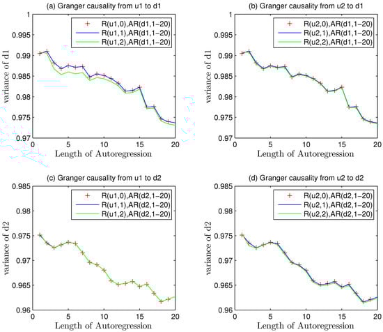
Figure 3.
The trend in the disturbance variance alteration in different channels without MPM.
The red line is merely corresponding to the variances of auto-regression mode. The blue curve describes just one step causality regression of and the green one gives a description of two step causality regressions.
Every part of four pictures in Figure 3 consists of three kinds of curves. The red-point curve implies the result of causality. The value of regression variance descends with the increase of auto-regression length, which is equivalent to the model order selection in system identification. Higher order can depict more details of the whole system but enhance the difficulty of controlling. It is necessary and reasonable to choose a proper size, like AIC criterion. As the nominal model is known to us, too high order is costly and unnecessary when it is greater than a convergent one. The biggest length of experiment is 20, which is enough to reveal the uniform convergence of auto-regression.
“Times” means the length of regression or auto regression coefficients, namely, the result of model order selection.
In view of the information in Table 3, the variance of white noise and that of were equal to 1, which played as a simplified noise benchmark in theory. But in real industrial, the variance is never just right the same as the set point value and always changing with data fluctuations. Sometimes the variance will be a little higher or lower than the designed one. The fluctuated value converges on the theoretical variance.
Table 3.
Explanations of labels in Figure 3.
The Equations (26) and (32) suggest that the variance of auto regression should be equal to that of pure white noise in each channel if no MPM occurred in this loop. However, Granger causality is a kind of regression methods that is based on statistical approaches so that overfitting of data is existing from start to finish. on the other hand, a lot of uncertainties in white noise make slight phenomenons. The first one is that the mean value of white noise is converging to zero but the real value is fluctuating nearby zero. The second one is that the variance is also converging and fluctuating around the theoretical value that equals 1 as designed.
From Theorem 4, the raise of model orders results in monotone increasing of Granger index. If curves do not coincide, such monotone increasing will cause regression curves to approach the benchmark line. Hence, model order should not be too high.
Figure 3 displayed the problems that statistical characteristics of and were approximately equal to theoretical value 1. In consideration of that the concept of overfitting and statistical fluctuation are inevitable, the results of variance could be accepted.
The model orders ware embodied in the lengths of auto regression about and . Too large order would lead to overfitting problems. Both of the two kind variances were gradually declining on the whole due to overfitting. Other than system identification, model orders were not so important as the causality. And to avoid the statistical interference in Granger analysis, upper and lower limits were adopted. If the causality regression results of or are within the limit lines, then the variance of will be regarded as equal with . The expectation of is almost the same with so that .
Similarly, it can be obtained that
4.1.2. Causality Compared with Decussation in Mismatch
The decussation method consists of two techniques, correlation analysis method between the input and the disturbance (CAID) and model quality index (MQI). Both methods can help to locate the MPM positions after coordination.
The process model varied from to .
Obviously, MPM occurred in Equation (92) and got mismatched in the system.
The data correlation between u1, the manipulated variable in first channel named and ds, the estimated noise in CAID algorithm, was below zero and its absolute value declined from 0.7071 to 0.4255 in Table 4 and Table 5. However, the correlation between u2 and ds also reduced. Besides, The MQI(2) was 0.9697 and similar to 1.0, which was as ideal as theoretical one.
Table 4.
Values of decussation under no MPM.
Table 5.
Values of decussation under mismatch.
The red and the blue curve that got coincidence in Figure 4a,b implies it may have no causality because the regression of dedicates no variance decrease to fault analyses. The scopes of variances are also below 1.0 close to 0.97 as the same condition of auto regression overfitting. Even the green curves describe some causality, and the scopes of variances are next to convergence value.
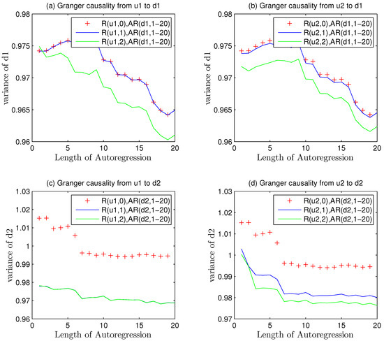
Figure 4.
The trend in the disturbance variance alteration in different channels under mismatch.
The Figure 4a,b reveals that in the first channel got no mismatch, which was under the same condition with that in Figure 3. The bottom pictures showed some differences and suggested the mismatch problems.
The sequence of is still composed of two parts. The first one is the disturbance noise as well as its transfer function . The other is the mismatched part, . Thus, the autoregression of would get larger than its theoretical values.
The variance of was above 1.0 in the beginning and got remarkable declines after Granger causality analysis.
The bottom two pictures (c)(d) in Figure 4 indicate that model plant mismatch exists in second channel but it is uncertain for the user to judge where the fault position is or whether two channels mismatch occurs together. To overcome these shortcomings, the assistant model of noise is introduced here.
The Equation (93) showed that causality in the second loop was larger than zero and the existence of mismatch was ensured.
A hint from Figure 5 implies that only model from u1 to the second channel mismatched. The average value in Figure 4 about data benchmark of the first five variances is 1.0122 and the mean value of causality is 0.9770. The decline of variance was caused by Granger regressions.
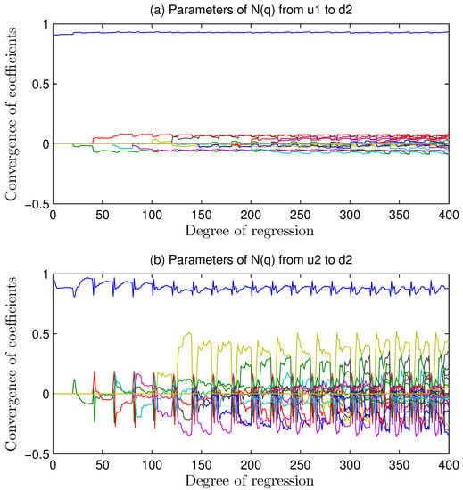
Figure 5.
Fluctuation of regression coefficients of assistant noise models estimated by GCA under mismatch.
Due to model mismatch in , the Granger index changed with this kind of interference. At this moment, consisted of two parts, the mismatch part as well as the noise part.
If got mismatched, the Granger causality index would reduce after regression analysis from to . Before regression method adopted, the sequence contained the mismatched information. After regression, the mismatched signal was extracted so that the left sequence contained nothing on and .
The top picture in Figure 5 reveals a better identification. The first coefficient of noise model in is 0.9. The maximum value in upper picture is almost 0.9, and the left coefficients are near to zero at the same time. The lower picture got a worse identification for misunderstanding. It was because that no matter or devoted nothing on mismatch that the extraction got wrong shapes. Considering increased more space for regression, the overfitting occurred.
The Figure 5a depicts a series of curves fluctuating slightly and converging to the theoretical values as noise transfer function. Better convergence effects than picture Figure 5b are because the regression of extracted most causality from the channel towards . The Figure 5b got bounding but only the facts that top line is equal to 0.9 as noise model set and the other parameters remains to be zero, embody correct regression. It was because the channel from towards devoted no causality to the MIMO systems that the regression in this channel did not know the mismatch condition. the causality algorithm forced it to overfit, and the parameters which are not near zero were not essential but once existed, would get over-fitted.
The convergence features of coefficients indicate the correct regression result from to and help to locate the channel i to j. Better convergence implies more reasonable regression and the less variance indicates the more significant Granger causality index. It is the real mismatched channel that reflects the occurrence of MPM so that the extraction of this channel information with regression technique can help to get a stable causality calculations. The index can quantify the fluctuations of parameters in .
Considering , the regression effects were in Figure 6 and Figure 7. All the parameters in Figure 6 were less than and its variances were less than , too. A better regression revealed the mismatch was from to , which showed that had a MPM problem.
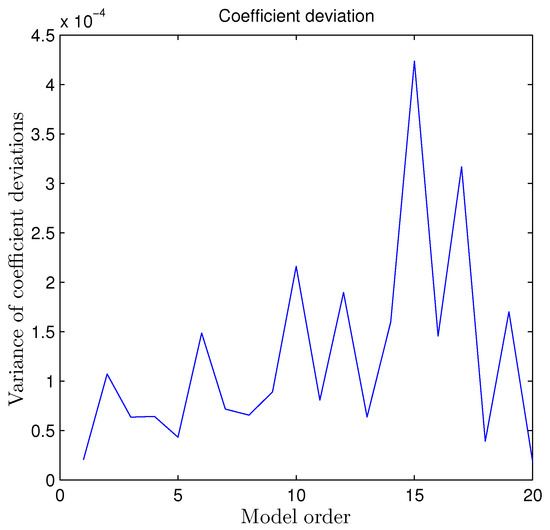
Figure 6.
Variance index of the amount of deviation from different model orders on regression coefficients under mismatch.
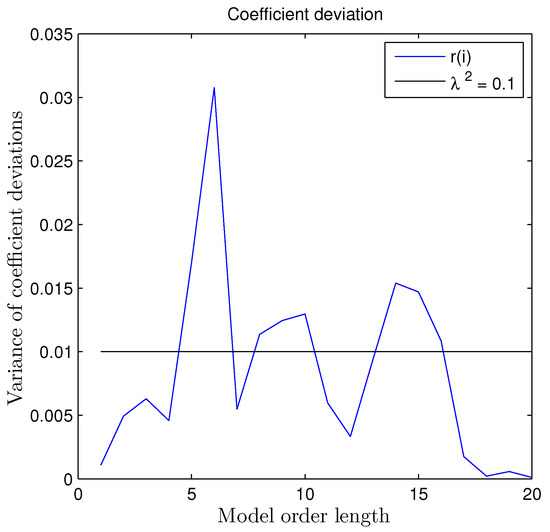
Figure 7.
Variance index of the amount of deviation from different model orders on regression coefficients under mismatch.
Among the 20 coefficients in Figure 7, eight of them were larger than and became over-limited. No mismatch plus regression method made this overfitting.
With the help of Equation (94), the location was finished and the mismatch position was from .
4.1.3. Causality Compared with Decussation in and Mismatches
In this section, two mismatches occurred in different channels. Besides, the mismatch positions in model parameters were also diverse. got its model mismatch in gain parts while became distinct in its denominator coefficient.
The decussation method showed that the significant declines of MQI(1) and CAID(u2,ds) pointed to the mismatch in , but bad effects on CAID(u1,ds) with good results of MQI(2) could not located the mismatch in .
CAID shows a negative influence of mismatches in both row channels. MQI(1) and CAID(u1,ds) locates an incorrect mismatch from to in Table 6. The reason is obvious, for data in MIMO system will get mutual interference. The information from and mismatches conducted to link and change the statistical characteristics, which caused erroneous judgment.
Table 6.
Values of decussation under and mismatch.
and mismatches had not been detected while the were wrongly judged. Besides, MQI(2) was seeming to normal but a little abnormal. If the judgment was correct, the mismatch would be missed. If the judgment was incorrect, then the four channels would get mismatched, which did not happen.
These suggest that decussation based on statistical correlation should be inaccurate, although it is a momentous means in analyzing the control loops.
Causalities in Figure 8 reveal all the channels got notable decreases in variances. It was possible that at least two mismatches existing in the closed loop system.
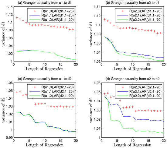
Figure 8.
The trend in the disturbance variance alteration in different channels under and mismatches.
The variance of auto regression of was 1.1 in Figure 8, suggesting that mismatch brought about worse Granger regression. And the variance of still got increased than before from 0.9939 to1.03.
Assistant model parameters would be,
and the locations of mismatch from to and another from to were ensured in view of Formula (98).
The Figure 9b,c shows a better convergence feature, which indicates two significant regression results from to and from to . Regression method extracts almost all mismatch information so that the left parameters of noise models are correct. The first coefficient of is converging to 0.8 and the second one to 0.9, which are consistent with Equation (88).
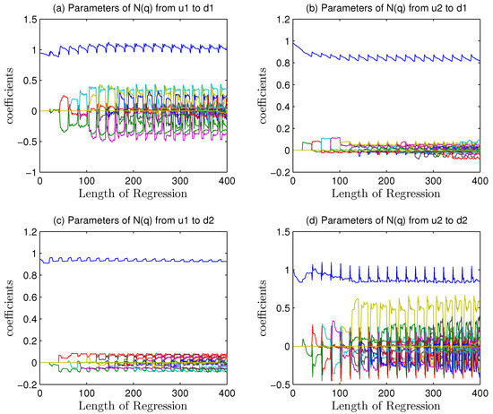
Figure 9.
Fluctuation of regression coefficients of assistant noise models estimated by GCA under and mismatch.
4.2. Quadruple-Tank Process
The quadruple-tank process that was comprehensively introduced by Johansson can be established and formed by two double-tank processes [29]. The process inputs consist of two voltages, and , as the input variables to control the pumps. Also the outputs and are voltage values collected from the level measurement in real systems. Mass balances and Bernoulli’s law must be obeyed to form the dynamic equations as follows.
Four dynamic functions are included in Equations (98), which explicates each liquid level of different tanks. Obviously, the dynamic functions are a series of nonlinear processes that should be dealt with before a proper controller is implemented in closed loops in Table 7.
Table 7.
Parameters of the quadruple-tank process.
The variable , , and represent the levels of four tanks, while the variable as well as reveals the condition of its corresponding valve.
Any output mainly contains the controlled object models as well as unmeasurable noise. So the output value can be unified and written as,
Therefore, all the outputs could be written in a whole matrix format.
The quadruple-tank process in this section is a four-input and four-output nonlinear system. The process must be linearized before implementing a suitable model predictive controller for this loop.
The linearized transfer functions are as below.
4.2.1. Complex Inputs: Both Setpoint Change and Zone Control in the Loops
as the first setpoint of the systems, encounters a rise from 8 to 23 at the time of 200th step of sampling time. is not a constant parameter and its functional relationship is sinusoidal with amplitude 12 and frequency 0.05 rad/s in Table 8. The fourth setpoint values are limited in a special zone so that the absolute values of its real input sequences are within −9 and 9 in Figure 10.
Table 8.
Setpoint conditions of the quadruple-tank process.
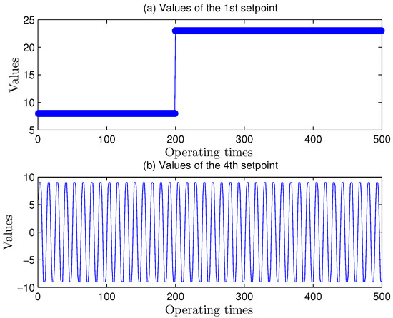
Figure 10.
Change laws of the 1st and the 4th Setpoint Values.
4.2.2. No Model Mismatch under Complex Inputs
The MIMO system was implemented by a linear MPC with the help of the software (Model Predictive Control Toolbox in MATLAB) under two complex inputs.
All the variances are less than the initial white noise sequence ones that equal to 1.000. Besides, the red-point line was almost in coincidence with the blue curve as well as the green curve in Figure 11. These two phenomena hinted that a few over-fittings of every white noise signal in light degrees existed on four channels, which implied that there was no model plant mismatch in this system.
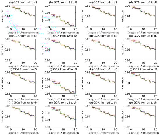
Figure 11.
Granger causality analyses of MIMO systems in different channels.
4.2.3. Higher Order Mismatch in
The transfer function in channel alters to
The Figure 12e–h presents different conditions from those in Figure 11. The variances are more than 1.000, which shows that there exists mismatch state in at least one channel in the second loop.
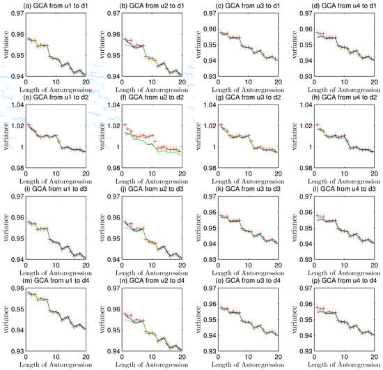
Figure 12.
Granger causality analyses of higher order mismatch in .
The three curves in Figure 12e–h are almost in coincidence, while the picture in Figure 12f reveals a little Granger causality.
The remaining pictures of Figure 12 show that there is no mismatch in the first, the third and the fourth loop in the whole system. The ranges of variances in Figure 12 are between 0.97 and 0.93 while those in Figure 11 varies from 0.96 to 0.92.
To further locate the mismatch channel, the assistance of disturbance transfer function models were carried out.
The disorder regressions in Figure 13b,d reveal that these two channels have no mismatch so that the regression effects are in divergence modes.
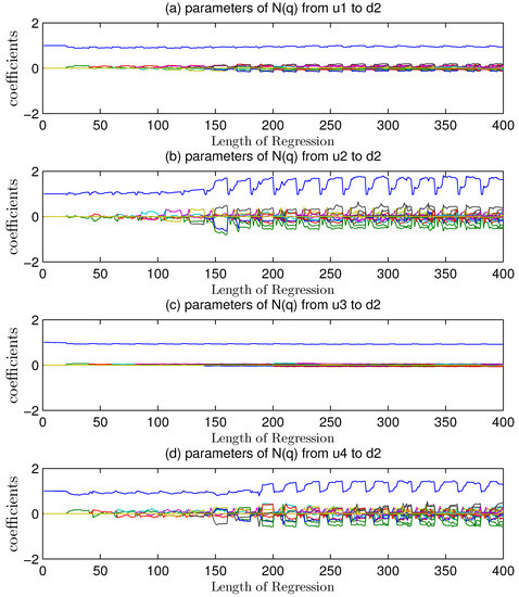
Figure 13.
Fluctuation of regression coefficients of assistant noise models estimated by GCA under higher order mismatch in .
The fluctuation of Figure 13a,c are not as obvious as the condition above, which implies that MPM might occur.
Considering the causality analysis would lead to some inaccuracy in location, the assistant model parameters would be needed.
The result shows the occurrence of mismatch.
4.2.4. Integral Mismatch in
When the process had an integral changes in some channels, the model structure would be changed. The object model had an integral mismatch as below,
MPC is a kind of controller based on the model structures, parameters and the degree of model accuracy. When an integral mismatch arose in channel, the object plant had a different structure from the nominal model, which was designed and tuned by the initial model predictive controller. Therefore, this alteration added some instability into the system and resulted in divergence of all the outputs in Figure 14.
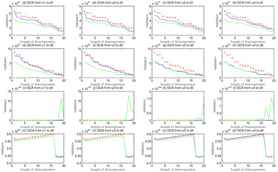
Figure 14.
Granger causality analyses of integral mismatch in .
When any loop in the system is not stable as daily routine, the operating data of the processes can not be used to analyze the condition effectively.
(i) If the integral section is not existing in the nominal models and it occurs in a model plant mismatch mode, the system will have a higher probability to be unstable and the instability will prevent the engineers from analyzing the mismatch.
(ii) If the integral section is always existing, the mismatch conditions about its parameter changes that do not affect the stability will be the same as those under Granger causality analysis.
4.2.5. Zero Gain Mismatch in
Some channel will have zero gain module, which means that this manipulated variable influences nothing towards the corresponding loop. However, some zero gain will disappear in the future so that the object model is not nought. Also, this kind of mismatch condition must obey the rule that the MPM should not affect the system stability.
Pictures in the third lines of Figure 15 and the third picture of Figure 16c imply that there is a mismatch in the channel.
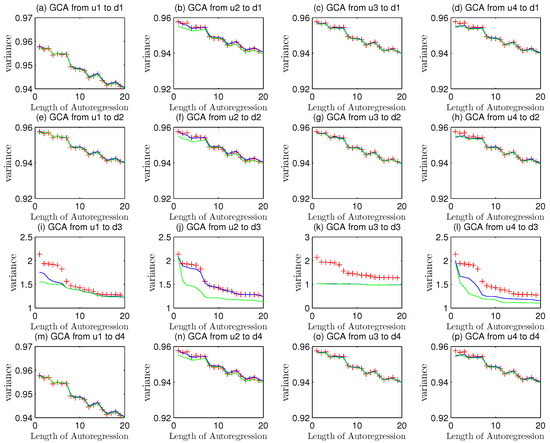
Figure 15.
Granger causality analyses of zero gain mismatch in .
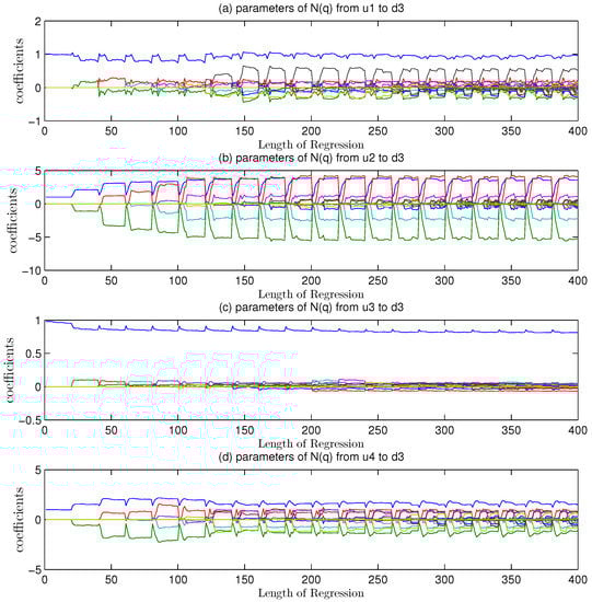
Figure 16.
Fluctuation of regression coefficients of assistant noise models estimated by GCA under zero gain mismatch in .
The result reveals the occurrence of mismatched model in the channel .
The monitored variances in pictures of Figure 17a,b,d are larger than 0.1 in the third loop and these data indicate a poor regression result from no mismatch parts. The picture of Figure 17c is less than 0.1 as expected, which is in accordance with the calculation in Equation (109). The location of this mismatch was finished with the assistant noise models.
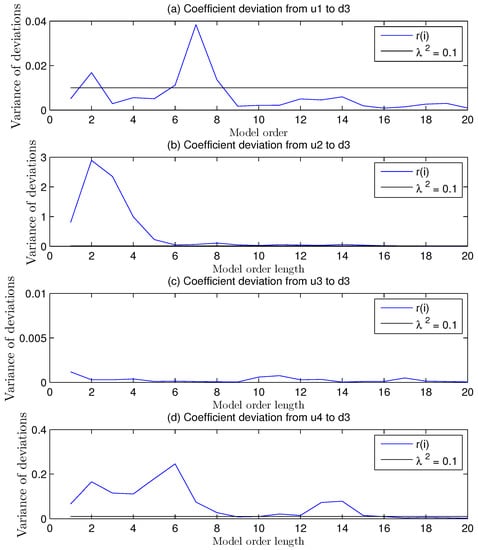
Figure 17.
Variance index of the amount of deviation from different model orders on regression coefficients under zero gain mismatch in .
5. Conclusions
Granger causality analysis can be used to detected the mismatch in closed loop system and obtain better results and accuracy from operating data in contrast to decussation location method using CAID and MQI. The decussation technique was implemented with statistical correlation methods and it was easily affected by mutual interference of control loops.
Granger causality analysis can provide for the users an explicit feedback whether the channels are influenced by MPM problems or not. The condition that causality index is greater than zero reflects a possible mismatch signal in the channel from manipulated variables to system output variables . However, once the mismatch conditions become complicated, the Granger causality as well as most MPM detection methods cannot guarantee the location of MPM.
To get further location of model plant mismatch, the assistant model parameters of white noise transfer function was introduced. When the mismatch occurred in specific channel from to , the regression of would contribute to the decrease of variance and the increase of Granger index. In the meantime, the assistant model parameters would get better identification so that coefficient deviation would become very little. Variables could be a monitoring tool for location.
The assistance of remaining noise models theoretically contain only noise sequences when there is no MPM occurence. However, mismatch leads to failure of 100 percent information extractions of process models so that the remaining noise models consist of two parts, the noise information and mismatched model features. This would result in the causality between and . Hence, Granger causality is adopted for detection as mentioned before. To test the remaining noise models compared with , the assistance of noise models can locate the real channels. When regression coefficients got exact results, it meant contained some information about , which reveals the fact that this channel got its mismatch. While the regression coefficients got the wrong estimation of process model, it shows that overfitting of variables towards and further describes the ruleless fitting of no mismatch variables, which demonstrates no mismatch in this channel but existence mismatch in system. This information provides the user to detect other channels to get the correct location.
Author Contributions
Conceptualization, M.C. and L.X.; methodology M.C. and L.X.; software, M.C.; validation, M.C.; formal analysis, M.C.; investigation, M.C. and L.X.; resources, M.C., L.X. and H.S.; data curation, M.C.; writing—original draft preparation, M.C.; writing—review and editing, M.C. and L.X.; visualization, M.C.; supervision, M.C. and L.X.; project administration, L.X.; funding acquisition, L.X. and H.S. All authors have read and agreed to the published version of the manuscript.
Funding
This research was funded by National Key R&D Program of China(No.2018YFB1701102), National Natural Science Foundation of P.R. China(NSFC:62073286) and Supported by Science Fund for Creative Research Groups of the National Natural Science Foundation of China (Grant No.61621002).
Institutional Review Board Statement
Not applicable.
Informed Consent Statement
Not applicable.
Data Availability Statement
Not applicable.
Conflicts of Interest
The authors declare no conflict of interests.
Abbreviations
The following abbreviations are used in this manuscript:
| CAID | Correlation Analysis method between the Input and the Disturbance |
| CPA | Control Performance Assessment |
| CV | Control Variables |
| GCA | Granger Causality Analysis |
| IMC | Internal Model Control |
| MIMO | Multiple Input Multiple Output |
| MPC | Model Predictive Control |
| MPM | Model Plant Mismatch |
| MQI | Model Quality Index |
| MVB | Minimum Variance Benchmark |
| MV | Manipulated Variables |
| PID | Proportional-Integral-Differential |
| ZOH | zero order holder |
References
- Claro, É.R.P.; de Oliveira Francisco, D.; Botelho, V.R.; Farenzena, M.; Trierweiler, J.O. Locating poor models in MPC applications. Comput. Chem. Eng. 2019, 130, 106545. [Google Scholar] [CrossRef]
- Wang, S.; Simkoff, J.M.; Baldea, M.; Chiang, L.H.; Castillo, I.; Bindlish, R.; Stanley, D.B. Autocovariance-based plant-model mismatch estimation for linear model predictive control. Syst. Control Lett. 2017, 104, 5–14. [Google Scholar] [CrossRef] [Green Version]
- Simkoff, J.M.; Wang, S.; Baldea, M.; Chiang, L.H.; Castillo, I.; Bindlish, R.; Stanley, D.B. Plant–Model Mismatch Estimation from Closed-Loop Data for State-Space Model Predictive Control. Ind. Eng. Chem. Res. 2018, 57, 3732–3741. [Google Scholar] [CrossRef]
- Badwe, A.S.; Gudi, R.D.; Patwardhan, R.S.; Shah, S.L.; Patwardhan, S.C. Detection of model-plant mismatch in MPC applications. J. Process. Control 2009, 19, 1305–1313. [Google Scholar] [CrossRef]
- Yerramilli, S.; Tangirala, A.K. Detection and diagnosis of model-plant mismatch in multivariable model-based control schemes. J. Process. Control 2018, 66, 84–97. [Google Scholar] [CrossRef]
- Yin, F.; Wang, H.; Xie, L.; Wu, P.; Song, Z.H. Data driven model mismatch detection based on statistical band of Markov parameters. Comput. Electr. Eng. 2014, 40, 2178–2192. [Google Scholar] [CrossRef]
- Wang, H.; H’Gglund, T.; Song, Z. Quantitative Analysis of Influences of Model Plant Mismatch on Control Loop Behavior. Ind. Eng. Chem. Res. 2012, 51, 15997–16006. [Google Scholar] [CrossRef]
- Khorasgani, H.; Farahat, A.; Ristovski, K.; Gupta, C.; Biswas, G. Framework for Unifying Model-based and Data-driven Fault Diagnosis. In Proceedings of the Annual Conference of the Prognostics and Health Management Society, Philadelphia, PA, USA, 24–27 September 2018; Volume 10. [Google Scholar] [CrossRef]
- Harris, T.J.; Boudreau, F.; MacGregor, J.F. Performance assessment of multivariable feedback controllers. Automatica 1996, 32, 1505–1518. [Google Scholar] [CrossRef]
- Rogozinski, M.; Paplinski, A.; Gibbard, M. An algorithm for the calculation of a nilpotent interactor matrix for linear multivariable systems. IEEE Trans. Autom. Control 1987, 32, 234–237. [Google Scholar] [CrossRef]
- Huang, B.; Ding, S.X.; Thornhill, N. Practical solutions to multivariate feedback control performance assessment problem: Reduced a priori knowledge of interactor matrices. J. Process. Control 2005, 15, 573–583. [Google Scholar] [CrossRef] [Green Version]
- Jie, Y.; Qin, S.J. MIMO control performance monitoring using left/right diagonal interactors. J. Process. Control 2009, 19, 1267–1276. [Google Scholar] [CrossRef]
- Yousefi, M.; Gopaluni, R.B.; Loewen, P.D.; Forbes, M.G.; Dumont, G.A.; Backstro, J. Impact of model plant mismatch on performance of control systems: An application to paper machine control. Control Eng. Pract. 2015, 43, 59–68. [Google Scholar] [CrossRef]
- Chen, M.; Xie, L.; Su, H. Impact of Model-Plant Mismatch to Minimum Variance Benchmark in Control Performance Assessment. In Proceedings of the 2020 39th Chinese Control Conference (CCC), Shenyang, China, 27–29 July 2020; pp. 2252–2257. [Google Scholar] [CrossRef]
- Badwe, A.S.; Patwardhan, R.S.; Shah, S.L.; Patwardhan, S.C.; Gudi, R.D. Quantifying the impact of model-plant mismatch on controller performance. J. Process. Control 2010, 20, 408–425. [Google Scholar] [CrossRef]
- Kaw, S.; Tangirala, A.K.; Karimi, A. Improved methodology and set-point design for diagnosis of model-plant mismatch in control loops using plant-model ratio. J. Process. Control 2014, 24, 1720–1732. [Google Scholar] [CrossRef]
- Ji, G.; Zhang, K.; Zhu, Y. A method of MPC model error detection. J. Process. Control 2012, 22, 635–642. [Google Scholar] [CrossRef]
- Zhao, J.; Zhu, Y.; Patwardhan, R. Identification of k-step-ahead prediction error model and MPC control. J. Process. Control 2014, 24, 48–56. [Google Scholar] [CrossRef]
- Kumar, D.M.D.; Narasimhan, S.; Bhatt, N. Detection of model-plant mismatch and model update for reaction systems using concept of extents. J. Process. Control 2018, 72, 17–29. [Google Scholar] [CrossRef]
- Webber, J.R.; Gupta, Y.P. A closed-loop cross-correlation method for detecting model mismatch in MIMO model-based controllers. Isa Trans. 2008, 47, 395–400. [Google Scholar] [CrossRef] [PubMed]
- Badwe, A.S.; Shah, S.L.; Patwardhan, S.C.; Patwardhan, R.S. Model-Plant Mismatch Detection in MPC Applications Using Partial Correlation Analysis. IFAC Proc. Vol. 2008, 41, 14926–14933. [Google Scholar] [CrossRef] [Green Version]
- Wang, S.; Simkoff, J.M.; Baldea, M.; Chiang, L.H.; Castillo, I.; Bindlish, R.; Stanley, D.B. Autocovariance-based MPC model mismatch estimation for systems with measurable disturbances. J. Process. Control 2017, 55, 42–54. [Google Scholar] [CrossRef]
- Botelho, V.; Trierweiler, J.O.; Farenzena, M.; Duraiski, R. Methodology for Detecting Model-Plant Mismatches Affecting Model Predictive Control Performance. Ind. Eng. Chem. Res. 2015, 54, 12072–12085. [Google Scholar] [CrossRef]
- Ling, D.; Zheng, Y.; Zhang, H.; Yang, W.; Tao, B. Detection of model-plant mismatch in closed-loop control system. J. Process. Control 2017, 57, 66–79. [Google Scholar] [CrossRef]
- Li, L.; Song, J.; Zhang, X.; Ye, J.; Yang, S. Model Deficiency Diagnosis and Improvement via Model Residual Assessment in Model Predictive Control. Ind. Eng. Chem. Res. 2017, 56, 12151–12162. [Google Scholar] [CrossRef]
- Li, L.; Lu, L.; Huang, Z.; Chen, X.; Yang, S. A model mismatch assessment method of MPC by decussation. Isa Trans. 2020, 106, 51–60. [Google Scholar] [CrossRef] [PubMed]
- Ren, W.; Li, B.; Han, M. A novel Granger causality method based on HSIC-Lasso for revealing nonlinear relationship between multivariate time series. Phys. A Stat. Mech. Its Appl. 2020, 541, 123245. [Google Scholar] [CrossRef]
- Seth, A.K. Granger causality. Scholarpedia 2007, 2, 1667. [Google Scholar] [CrossRef]
- Johansson, K.H. The quadruple-tank process: A multivariable laboratory process with an adjustable zero. IEEE Trans. Control Syst. Technol. 2000, 8, 456–465. [Google Scholar] [CrossRef] [Green Version]
Publisher’s Note: MDPI stays neutral with regard to jurisdictional claims in published maps and institutional affiliations. |
© 2021 by the authors. Licensee MDPI, Basel, Switzerland. This article is an open access article distributed under the terms and conditions of the Creative Commons Attribution (CC BY) license (https://creativecommons.org/licenses/by/4.0/).