
Variable Neighborhood Strategy Adaptive Search for Optimal Parameters of SSM-ADC 12 Aluminum Friction Stir Welding


 ,
,  , ,
, , 
Abstract
:1. Introduction
2. Literature Review
3. Materials and Methods
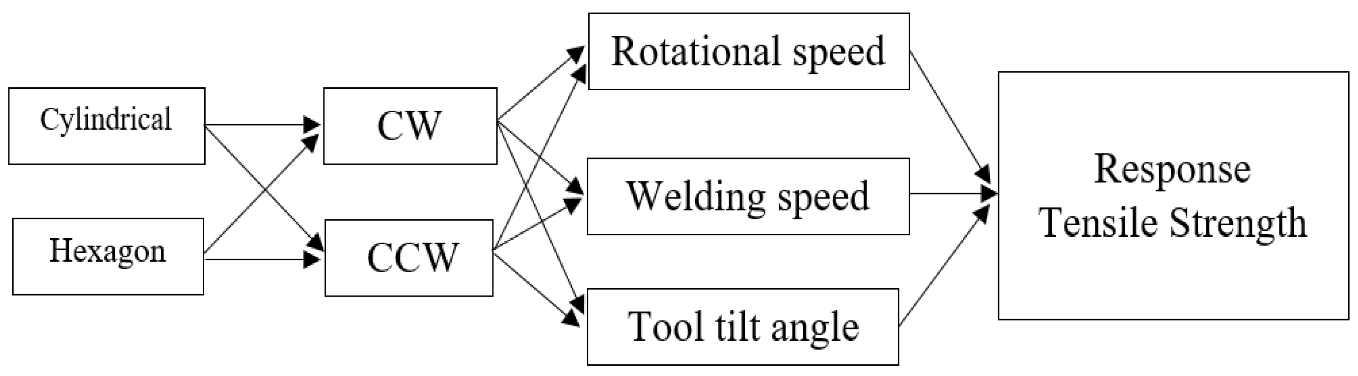
3.1. Identifying the Number of Parameters of Interest and Their Ranges and Levels
3.2. Using D-Optimal Experimental Design to Find the Regression Model of the Parameters for Friction Stir Welding
3.3. Using Variable Neighborhood Strategy Adaptive Search to Find the Optimal Parameters
3.3.1. Generate a Set of Tracks
3.3.2. Perform Track Touring Process in a Specified Black Box
3.3.3. Black Box Operation
K-Exchange Method (KEM)
K-Transition Method (KTM)
3.3.4. Update the Track
3.3.5. Repeat the Steps
3.4. The Methods Compared
3.4.1. Differential Evolution Algorithm (DE)
3.4.2. Genetic Algorithm (GA)
4. Experimental Framework and Results
4.1. Optimization Process by D-Optimal Experimental Design
4.2. Results Using Variable Neighborhood Strategy Adaptive Search (VaNSAS)
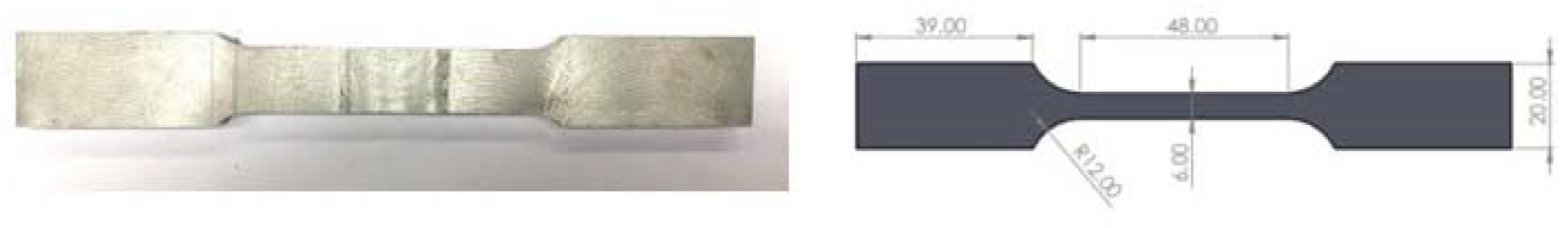
4.3. Verifying the Results by Testing Optimal Parameters with Actual Specimens
4.4. The Reliability and Effectiveness Testing of the Proposed Methods
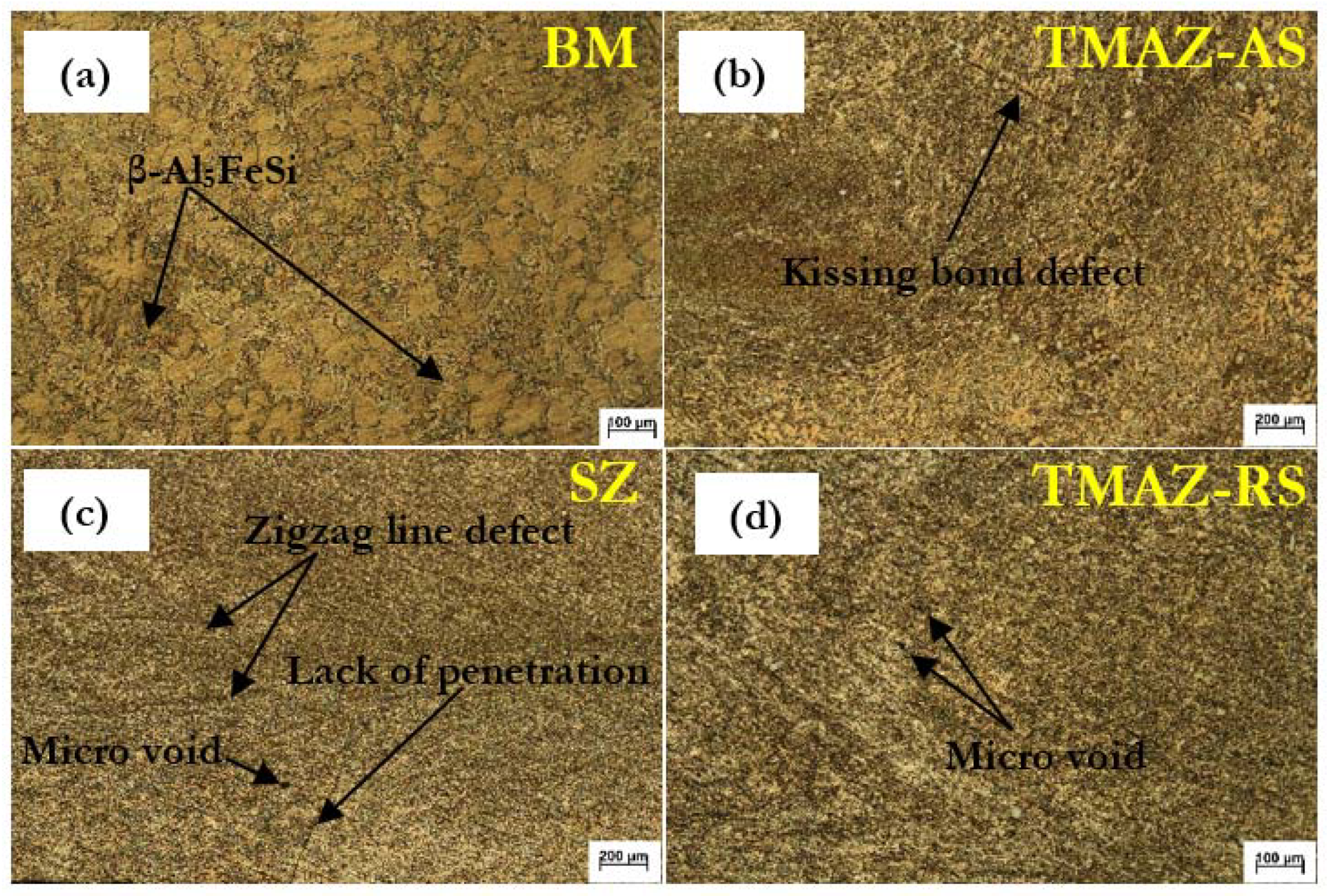
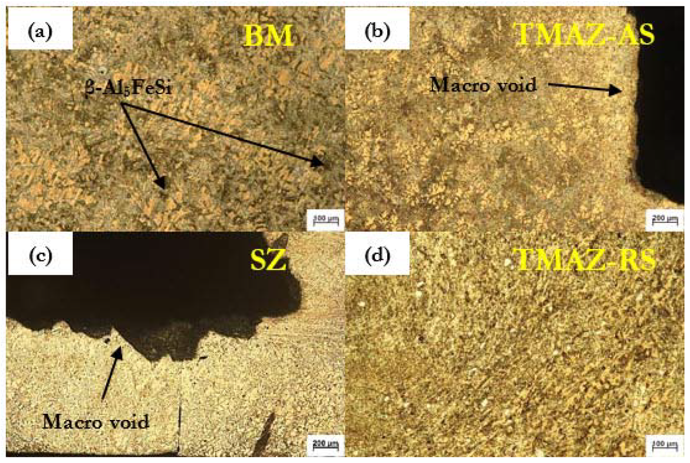
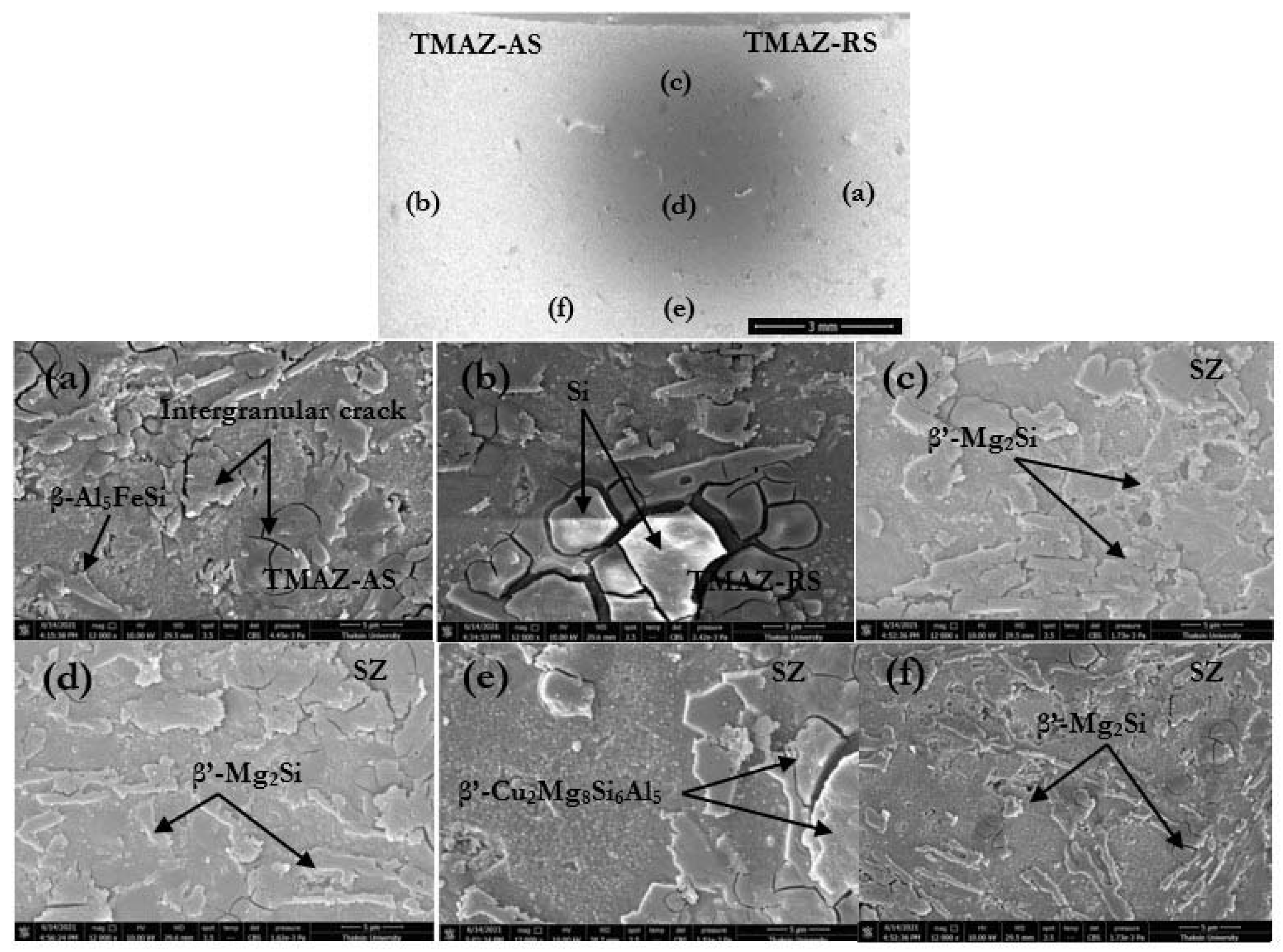
4.5. Microstructure Analysis
5. Conclusions
Author Contributions
Funding
Institutional Review Board Statement
Informed Consent Statement
Data Availability Statement
Acknowledgments
Conflicts of Interest
Appendix A

| Track Number | Current Track Track 1 | Randomly Selected Track Track 2 | New Track Track 1 |
|---|---|---|---|
| Element | |||
| 1 (Rotational speed) | 0.36 | 0.74 | 0.74 |
| 2 (Welding speed) | 0.71 | 0.32 | 0.71 |
| 3 (Tool tilt angle) | 0.20 | 0.03 | 0.03 |
Appendix B
| Track Number | Current Track Track 1 (1) | Random Number (2) | New Track Track 1 (3) |
|---|---|---|---|
| Element | |||
| 1 (Rotational speed) | 0.36 | 0.45 | 0.36 |
| 2 (Welding speed) | 0.71 | 0.89 | 0.89 |
| 3 (Tool tilt angle) | 0.20 | 0.14 | 0.14 |
Appendix C. Pseudocode of VaNSAS
| Algorithm A1: Variable Neighborhood Strategy Adaptive Search (VaNSAS) |
| input:Number of Track (NP), Problem Size (D), Mutation Rate (F), Recombination rate (R), Number of Black box (NBB) |
| output: Best_Track_Solution |
| begin |
| Population = Initialize Track (NP, D) |
| IBPop = Initialize Information BB(NBB) |
| encode Population as a track |
| while the stopping criterion is not met do |
| for i = 1: NP |
| Set u [j] = randomnumber)_[j] |
| //selected black box by RouletteWheelSelection |
| selected_BB = RouletteWheelSelection(BBPop) using Equation (3) |
| If(selected_BB = 1) Then |
| new_u = SDE (u) |
| Else if(selected_BB = 2) |
| new_u = K-exchange (u) |
| Else if(selected_BB = 3) |
| new_u = K_Transition (u) |
| IF(CostFunction(new_u) ≤ CostFunction(Vi)) Then |
| Vi = new_u |
| //Loop for update heuristics information of Intelligence box |
| For j = 1: NBB |
| BBPopi using Equaltion (8) |
| End For Loop//end update heuristics information |
| End For Loop |
| End |
| Decode WP to get the solution for the problem |
| Return Best track Solution |
| end |
Appendix D. Pseudocode of DE
| Algorithm A2: Differential evolution algorithm (DE) |
| input:Population size (NP), Problem Size (D), Mutation Rate (F), Recombination rate (R) |
| output: Best_Vector_Solution |
| begin |
| Population = Initialize Population (NP, D) |
| encode Population to WP |
| while the stopping criterion is not met do |
| for i = 1: NP |
| Vrand1, Vrand2, Vrand3 = Select_Random_Vector (WP) |
| For j = 1: D//Loop for the mutation operator |
| Vy [j] = Vrand1 [j] + F (Vrand2 [j] + Vrand3 [j]) |
| End For Loop//end mutation operator |
| For j = 1: D//Loop for recombination operation |
| If (randj [0,1) < R) Then |
| u [j] = Vi [j] |
| Else |
| u [j] = Vy [j] |
| End For Loop//end recombination operation |
| IF(CostFunction(u) ≤ CostFunction(Vi)) Then |
| Vi = u |
| End For Loop |
| End |
| decode WP to get the solution for the problem |
| Return Best Vector Solution |
| end |
Appendix E. Pseudocode of GA
| Algorithm A3: Genetic Algorithm (GA) |
| input:Population Size (NP), Problem Size (D), Mutation Rate (M), Crossover Rate (CR) |
| output: Best_Vector_Solution |
| begin |
| Population = Initialize Population (NP, D) |
| encode Population to WP |
| while the stopping criterion is not met do |
| parents = WP |
| for i = 1: NP//Loop for crossover operation |
| For j = 1: D |
| If(randj [0,1) < CR ) Then |
| offspringi [j] = parentsi [j] |
| offspringi+1 [j] = parentsi+1 [j] |
| Else |
| offspringi [j] = parentsi+1 [j] |
| offspringi+1 [j] = parentsi [j] |
| End For Loop |
| End For Loop//end crossover operation |
| for i = 1: NP//Loop for mutation operation |
| For j = 1: D |
| If(randj [0,1) < M ) Then |
| Mutation(offspringi[j]) |
| End For Loop |
| End For Loop//end mutation operation |
| //Add the child population to the parent population |
| NWP = stack(parents, offspring) |
| wp_size = length(NWP)//Set number of new population |
| for i = 1: wp_size//Loop for evaluate operation |
| cost_ scores i+1= CostFunction(NWPi+1) |
| End For Loop//end evaluate operation |
| //selection operation |
| new_wp = Sorted(new_ population, cost_scores) |
| WP = NWP [1:NP] |
| decode WP to get the solution for the problem |
| Return Best Vector Solutionend |
| end |
References
- Jirang, C.; Roven, H.J. Recycling of automotive aluminum. Trans. Nonferrous Met. Soc. China 2010, 20, 2057–2063. [Google Scholar]
- Heinz, A.; Haszler, A.; Keidel, C.; Moldenhauer, S.; Benedictus, R.; Miller, W. Recent development in aluminium alloys for aerospace applications. Mater. Sci. Eng. A 2000, 280, 102–107. [Google Scholar] [CrossRef]
- Miller, W.; Zhuang, L.; Bottema, J.; Wittebrood, A.J.; De Smet, P.; Haszler, A.; Vieregge, A. Recent development in aluminium alloys for the automotive industry. Mater. Sci. Eng. A 2000, 280, 37–49. [Google Scholar] [CrossRef]
- Guo, H.; Hu, J.; Tsai, H.-L. Formation of weld crater in GMAW of aluminum alloys. Int. J. Heat Mass Transf. 2009, 52, 5533–5546. [Google Scholar] [CrossRef]
- Da Silva, C.L.M.; Scotti, A. The influence of double pulse on porosity formation in aluminum GMAW. J. Mater. Process. Technol. 2006, 171, 366–372. [Google Scholar] [CrossRef]
- Fang, X.; Zhang, J. Effect of underfill defects on distortion and tensile properties of Ti-2Al-1.5 Mn welded joint by pulsed laser beam welding. Int. J. Adv. Manuf. Technol. 2014, 74, 699–705. [Google Scholar] [CrossRef]
- Thomas, W.M.; Johnson, K.I.; Wiesner, C.S. Friction stir welding–recent developments in tool and process technologies. Adv. Eng. Mater. 2003, 5, 485–490. [Google Scholar] [CrossRef]
- Thomas, W.; Nicholas, E. Friction stir welding for the transportation industries. Mater. Des. 1997, 18, 269–273. [Google Scholar] [CrossRef]
- Threadgill, P.; Leonard, A.; Shercliff, H.; Withers, P. Friction stir welding of aluminium alloys. Int. Mater. Rev. 2009, 54, 49–93. [Google Scholar] [CrossRef]
- Lakshminarayanan, A.; Malarvizhi, S.; Balasubramanian, V. Developing friction stir welding window for AA2219 aluminium alloy. Trans. Nonferrous Met. Soc. China 2011, 21, 2339–2347. [Google Scholar] [CrossRef]
- Guo, J.; Chen, H.; Sun, C.; Bi, G.; Sun, Z.; Wei, J. Friction stir welding of dissimilar materials between AA6061 and AA7075 Al alloys effects of process parameters. Mater. Des. 2014, 56, 185–192. [Google Scholar] [CrossRef]
- Hoyos, E.; Escobar, S.; Backer, J.D.; Martin, J.; Palacio, M. Manufacturing Concept and Prototype for Train Component Using the FSW Process. J. Manuf. Mater. Process. 2021, 5, 19. [Google Scholar]
- Giraud, L.; Robe, H.; Claudin, C.; Desrayaud, C.; Bocher, P.; Feulvarch, E. Investigation into the dissimilar friction stir welding of AA7020-T651 and AA6060-T6. J. Mater. Process. Technol. 2016, 235, 220–230. [Google Scholar] [CrossRef]
- Bisadi, H.; Tavakoli, A.; Sangsaraki, M.T.; Sangsaraki, K.T. The influences of rotational and welding speeds on microstructures and mechanical properties of friction stir welded Al5083 and commercially pure copper sheets lap joints. Mater. Des. 2013, 43, 80–88. [Google Scholar] [CrossRef]
- Kadaganchi, R.; Gankidi, M.R.; Gokhale, H. Optimization of process parameters of aluminum alloy AA 2014-T6 friction stir welds by response surface methodology. Def. Technol. 2015, 11, 209–219. [Google Scholar] [CrossRef] [Green Version]
- Lotfi, A.H.; Nourouzi, S. Effect of welding parameters on microstructure, thermal, and mechanical properties of friction-stir welded joints of AA7075-T6 aluminum alloy. Metall. Mater. Trans. A 2014, 45, 2792–2807. [Google Scholar] [CrossRef]
- Khan, N.Z.; Khan, Z.A.; Siddiquee, A.N. Effect of shoulder diameter to pin diameter (D/d) ratio on tensile strength of friction stir welded 6063 aluminium alloy. Mater. Today Proc. 2015, 2, 1450–1457. [Google Scholar] [CrossRef]
- Liu, H.; Zhang, H.; Pan, Q.; Yu, L. Effect of friction stir welding parameters on microstructural characteristics and mechanical properties of 2219-T6 aluminum alloy joints. Int. J. Mater. Form. 2012, 5, 235–241. [Google Scholar] [CrossRef]
- Elangovan, K.; Balasubramanian, V. Influences of tool pin profile and welding speed on the formation of friction stir processing zone in AA2219 aluminium alloy. J. Mater. Process. Technol. 2008, 200, 163–175. [Google Scholar] [CrossRef]
- Li, W.; Li, J.; Zhang, Z.; Gao, D.; Wang, W.; Luan, G. Pinless friction stir welding of AA2024-T3 joint and its failure modes. Trans. Tianjin Univ. 2014, 20, 439–443. [Google Scholar] [CrossRef]
- Ilangovan, M.; Boopathy, S.R.; Balasubramanian, V. Effect of tool pin profile on microstructure and tensile properties of friction stir welded dissimilar AA 6061–AA 5086 aluminium alloy joints. Def. Technol. 2015, 11, 174–184. [Google Scholar] [CrossRef] [Green Version]
- Ghaffarpour, M.; Kolahgar, S.; Dariani, B.M.; Dehghani, K. Evaluation of dissimilar welds of 5083-H12 and 6061-T6 produced by friction stir welding. Metall. Mater. Trans. A 2013, 44, 3697–3707. [Google Scholar] [CrossRef]
- RajKumar, V.; VenkateshKannan, M.; Sadeesh, P.; Arivazhagan, N.; Ramkumar, K.D. Studies on effect of tool design and welding parameters on the friction stir welding of dissimilar aluminium alloys AA 5052–AA 6061. Procedia Eng. 2014, 75, 93–97. [Google Scholar] [CrossRef] [Green Version]
- Kasman, Ş.; Yenier, Z. Analyzing dissimilar friction stir welding of AA5754/AA7075. Int. J. Adv. Manuf. Technol. 2014, 70, 145–156. [Google Scholar] [CrossRef]
- Kesharwani, R.; Panda, S.; Pal, S. Multi objective optimization of friction stir welding parameters for joining of two dissimilar thin aluminum sheets. Procedia Mater. Sci. 2014, 6, 178–187. [Google Scholar] [CrossRef] [Green Version]
- Uematsu, Y.; Kakiuchi, T.; Tozaki, Y.; Kojin, H. Comparative study of fatigue behaviour in dissimilar Al alloy/steel and Mg alloy/steel friction stir spot welds fabricated by scroll grooved tool without probe. Sci. Technol. Weld. Join. 2012, 17, 348–356. [Google Scholar] [CrossRef]
- Ji, S.; Meng, X.; Ma, L.; Gao, S. Effect of groove distribution in shoulder on formation, macrostructures, and mechanical properties of pinless friction stir welding of 6061-O aluminum alloy. Int. J. Adv. Manuf. Technol. 2016, 87, 3051–3058. [Google Scholar] [CrossRef]
- Meengam, C.; Sillapasa, K. Evaluation of Optimization Parameters of Semi-Solid Metal 6063 Aluminum Alloy from Friction Stir Welding Process Using Factorial Design Analysis. J. Manuf. Mater. Process 2020, 4, 1–20. [Google Scholar]
- Koilraj, M.; Sundareswaran, V.; Vijayan, S.; Rao, S.K. Friction stir welding of dissimilar aluminum alloys AA2219 to AA5083–Optimization of process parameters using Taguchi technique. Mater. Des. 2012, 42, 1–7. [Google Scholar] [CrossRef]
- Srichok, T.; Pitakaso, R.; Sethanan, K.; Sirirak, W.; Kwangmuang, P. Combined Response Surface Method and Modified Differential Evolution for Parameter Optimization of Friction StirWelding. Processes 2020, 8, 1080. [Google Scholar] [CrossRef]
- Hartl, R.; Vieltorf, F.; Benker, M.; Zaeh, M.F. Predicting the Ultimate Tensile Strength of Friction Stir Welds Using Gaussian Process Regression. J. Manuf. Mater. Process 2020, 4, 75. [Google Scholar] [CrossRef]
- Prasad, M.D.; kumar Namala, K. Process parameters optimization in friction stir welding by ANOVA. Mater. Today Proc. 2018, 5, 4824–4831. [Google Scholar] [CrossRef]
- Shanavas, S.; Dhas, J.E.R. Parametric optimization of friction stir welding parameters of marine grade aluminium alloy using response surface methodology. Trans. Nonferrous Met. Soc. China 2017, 27, 2334–2344. [Google Scholar] [CrossRef]
- Hartl, R.; Praehofer, B.; Zaeh, M. Prediction of the surface quality of friction stir welds by the analysis of process data using Artificial Neural Networks. Proc. Inst. Mech. Eng. Part L J. Mater. Des. Appl. 2020, 234, 732–751. [Google Scholar] [CrossRef]
- Bayazid, S.; Farhangi, H.; Ghahramani, A. Investigation of friction stir welding parameters of 6063-7075 aluminum alloys by Taguchi method. Procedia Mater. Sci. 2015, 11, 6–11. [Google Scholar] [CrossRef] [Green Version]
- Shojaeefard, M.H.; Akbari, M.; Asadi, P. Multi objective optimization of friction stir welding parameters using FEM and neural network. Int. J. Precis. Eng. Manuf. 2014, 15, 2351–2356. [Google Scholar] [CrossRef]
- Teimouri, R.; Baseri, H. Forward and backward predictions of the friction stir welding parameters using fuzzy-artificial bee colony-imperialist competitive algorithm systems. J. Intell. Manuf. 2015, 26, 307–319. [Google Scholar] [CrossRef]
- Roshan, S.B.; Jooibari, M.B.; Teimouri, R.; Asgharzadeh-Ahmadi, G.; Falahati-Naghibi, M.; Sohrabpoor, H. Optimization of friction stir welding process of AA7075 aluminum alloy to achieve desirable mechanical properties using ANFIS models and simulated annealing algorithm. Int. J. Adv. Manuf. Technol. 2013, 69, 1803–1818. [Google Scholar] [CrossRef]
- Aydin, H.; Bayram, A.; Esme, U.; Kazancoglu, Y.; Guven, O. Application of Grey Relation Analysis (GRA) and Taguchi Method for the Parametric Optimization of Friction Stir Welding (FSW) Process. Mater. Technol. 2010, 44, 205–211. [Google Scholar]
- Tansel, I.N.; Demetgul, M.; Okuyucu, H.; Yapici, A. Optimizations of friction stir welding of aluminum alloy by using genetically optimized neural network. Int. J. Adv. Manuf. Technol. 2010, 48, 95–101. [Google Scholar] [CrossRef] [Green Version]
- Lakshminarayanan, A.; Balasubramanian, V. Process parameters optimization for friction stir welding of RDE-40 aluminium alloy using Taguchi technique. Trans. Nonferrous Met. Soc. China 2008, 18, 548–554. [Google Scholar] [CrossRef]
- Yousif, Y.K.; Daws, K.M.; Kazem, B.I. Prediction of Friction Stir Welding Characteristic Using Neural Network. Jordan J. Mech. Ind. Eng. 2008, 2, 151–155. [Google Scholar]
- Mao, Y.; Ke, L.; Liu, F.; Huang, C.; Chen, Y.; Liu, Q. Effect of welding parameters on microstructure and mechanical properties of friction stir welded joints of 2060 aluminum lithium alloy. Int. J. Adv. Manuf. Technol. 2015, 81, 1419–1431. [Google Scholar] [CrossRef]
- Zimmer, S.; Langlois, L.; Laye, J.; Goussain, J.-C.; Martin, P.; Bigot, R. Influence of processing parameters on the tool and workpiece mechanical interaction during Friction Stir Welding. Int. J. Mater. 2009, 2, 299–302. [Google Scholar] [CrossRef] [Green Version]
- Jassim, A.K.; Ali, D.C.; Barak, A. Effect of tool rotational direction and welding speed on the quality of friction stir welded Al-Mg Alloy 5052-O. J. Appl. Sci. Eng. 2018, 13, 2352–2358. [Google Scholar]
- Panneerselvam, K.; Lenin, K. Joining of Nylon 6 plate by friction stir welding process using threaded pin profile. Mater. Des. 2014, 53, 302–307. [Google Scholar] [CrossRef]
- Chen, J.; Fujii, H.; Sun, Y.; Morisada, Y.; Kondoh, K. Effect of material Flow by double-sided fsw on mechanical properties of mg alloys. In Proceedings of the National Meeting of JWS 2011, Iseshi, Japan, 7–9 September 2011; pp. 134–135. [Google Scholar]
- Fu, R.; Ji, H.; Li, Y.; Liu, L. Effect of weld conditions on microstructures and mechanical properties of friction stir welded joints on AZ31B magnesium alloys. Sci. Technol. Weld. Join. 2012, 17, 174–179. [Google Scholar] [CrossRef]
- Fu, R.; Sun, R.; Zhang, F.; Liu, H. Improvement of formation quality for friction stir welded joints. Weld. J. 2012, 91, 169–173. [Google Scholar]
- Kuram, E.; Ozcelik, B.; Bayramoglu, M.; Demirbas, E.; Simsek, B.T. Optimization of cutting fluids and cutting parameters during end milling by using D-optimal design of experiments. J. Clean. Prod. 2013, 42, 159–166. [Google Scholar] [CrossRef]
- Jones, B.; Allen-Moyer, K.; Goos, P. A-optimal versus D-optimal design of screening experiments. J. Qual. Technol. 2020, 53, 1–14. [Google Scholar] [CrossRef]
- Ba-Abbad, M.M.; Kadhum, A.A.H.; Mohamad, A.B.; Takriff, M.S.; Sopian, K. Optimization of process parameters using D-optimal design for synthesis of ZnO nanoparticles via sol–gel technique. J. Ind. Eng. Chem. 2013, 19, 99–105. [Google Scholar] [CrossRef]
- Theeraviriya, C.; Ruamboon, K.; Praseeratasang, N. Solving the multi-level location routing problem considering the environmental impact using a hybrid metaheuristic. Int. J. Eng. Bus. Manag. 2021, 13, 18479790211017353. [Google Scholar] [CrossRef]
- Theeraviriya, C.; Sirirak, W.; Praseeratasang, N. Location and routing planning considering electric vehicles with restricted distance in agriculture. World Electr. Veh. J. 2020, 11, 61. [Google Scholar] [CrossRef]
- Khamsing, N.; Chindaprasert, K.; Pitakaso, R.; Sirirak, W.; Theeraviriya, C. Modified ALNS Algorithm for a Processing Application of Family Tourist Route Planning: A Case Study of Buriram in Thailand. Computation 2021, 9, 23. [Google Scholar] [CrossRef]
- Kusoncum, C.; Sethanan, K.; Pitakaso, R.; Hartl, R.F. Heuristics with novel approaches for cyclical multiple parallel machine scheduling in sugarcane unloading systems. Int. J. Prod. Res. 2021, 59, 2479–2497. [Google Scholar] [CrossRef]
- Jirasirilerd, G.; Pitakaso, R.; Sethanan, K.; Kaewman, S.; Sirirak, W.; Kosacka-Olejnik, M. Simple Assembly Line Balancing Problem Type 2 by Variable Neighborhood Strategy Adaptive Search: A Case Study Garment Industry. J. Open Innov. Technol. Mark. Complex. 2020, 6, 21. [Google Scholar] [CrossRef] [Green Version]
- Pitakaso, R.; Sethanan, K.; Theeraviriya, C. Variable neighborhood strategy adaptive search for solving green 2-echelon location routing problem. Comput. Electron. Agric. 2020, 173, 105406. [Google Scholar] [CrossRef]
- Cisko, A.; Jordon, J.; Amaro, R.; Allison, P.; Wlodarski, J.; McClelland, Z.; Garcia, L.; Rushing, T. A parametric investigation on friction stir welding of Al-Li 2099. Mater. Manuf. Process. 2020, 35, 1069–1076. [Google Scholar] [CrossRef]
- Tehyo, M.; Muangjunburee, P.; Chuchom, S. Friction stir welding of dissimilar joint between semi-solid metal 356 and AA 6061-T651 by computerized numerical control machine. Songklanakarin J. Sci. Technol. 2011, 33, 441–448. [Google Scholar]
- Palani, K.; Elanchezhian, C.; Ramnath, B.V.; Bhaskar, G.B. Modeling and Optimization of FSW Parameters on Tensile Behavior of Aluminium Alloys using D-Optimal Design. Adv. Sci. Eng. Med. 2018, 10, 384–389. [Google Scholar] [CrossRef]
- Suenger, S.; Kreissle, M.; Kahnert, M.; Zaeh, M.F. Influence of Process Temperature on Hardness of Friction Stir Welded High Strength Aluminum Alloys for Aerospace Applications. Procedia CIRP 2014, 24, 120–124. [Google Scholar] [CrossRef] [Green Version]
- Eren, B.; Guvenc, M.A.; Mistikoglu, S. Artificial intelligence applications for friction stir welding: A review. Met. Mater. Int. 2021, 27, 193–219. [Google Scholar] [CrossRef]
- Pitakaso, R.; Sethanan, K.; Jirasirilerd, G.; Golinska-Dawson, P. A novel variable neighborhood strategy adaptive search for SALBP-2 problem with a limit on the number of machine’s types. Ann. Oper. Res. 2021, 298, 1–25. [Google Scholar]
- Myers, R.H.; Montgomery, D.C.; Anderson-Cook, C. Process and product optimization using designed experiments. Response Surf. Methodol. 2002, 2, 328–335. [Google Scholar]
- Mitchell, M. An Introduction to Genetic Algorithms; MIT Press: Cambridge, MA, USA, 1996. [Google Scholar]
- Su, J.-L.; Wang, H. An improved adaptive differential evolution algorithm for single unmanned aerial vehicle multitasking. Def. Technol. 2021. [Google Scholar] [CrossRef]
- Hoogervorst, R.; Dollevoet, T.; Maróti, G.; Huisman, D. A Variable Neighborhood Search heuristic for rolling stock rescheduling. EURO J. Transp. Logist. 2021, 10, 100032. [Google Scholar] [CrossRef]
- Chen, J.; Dan, B.; Shi, J. A variable neighborhood search approach for the multi-compartment vehicle routing problem with time windows considering carbon emission. J. Clean. Prod. 2020, 277, 123932. [Google Scholar] [CrossRef]
- Muñoz, A.; Rubio, F. Evaluating genetic algorithms through the approximability hierarchy. J. Comput. Sci. 2021, 53, 101388. [Google Scholar] [CrossRef]
- Jenarthanan, M.; Varma, C.V.; Manohar, V.K. Impact of friction stir welding (FSW) process parameters on tensile strength during dissimilar welds of AA2014 and AA6061. Mater. Today Proc. 2018, 5, 14384–14391. [Google Scholar] [CrossRef]
- Medhi, T.; Hussain, S.A.I.; Roy, B.S.; Saha, S.C. Selection of best process parameters for friction stir welded dissimilar Al-Cu alloy: A novel MCDM amalgamated MORSM approach. J. Braz. Soc. Mech. Sci. Eng. 2020, 42, 1–22. [Google Scholar] [CrossRef]
- Farzadi, A.; Bahmani, M.; Haghshenas, D. Optimization of operational parameters in friction stir welding of AA7075-T6 aluminum alloy using response surface method. Arab. J. Sci. Eng. 2017, 42, 4905–4916. [Google Scholar] [CrossRef]
- Ahmadnia, M.; Shahraki, S.; Kamarposhti, M.A. Experimental studies on optimized mechanical properties while dissimilar joining AA6061 and AA5010 in a friction stir welding process. Int. J. Adv. Manuf. Technol. 2016, 87, 2337–2352. [Google Scholar] [CrossRef]
- Sankar, B.R.; Umamaheswarrao, P. Modelling and optimisation of friction stir welding on AA6061 Alloy. Mater. Today Proc. 2017, 4, 7448–7456. [Google Scholar] [CrossRef]
- Singh, H.N.; Kaushik, A.; Juneja, D. Optimization of process parameters of friction stir welded joint of AA6061 and AA6082 by response surface methodology (RSM). Int. J. Res. Eng. Innov. 2019, 3, 417–427. [Google Scholar] [CrossRef]
- Goyal, A.; Garg, R.K. Establishing mathematical relationships to study tensile behavior of friction stir welded AA5086-H32 aluminium alloy joints. Silicon 2019, 11, 51–65. [Google Scholar] [CrossRef]
- Jannet, S.; Mathews, P.K.; Raja, R. Optimization of process parameters of friction stir welded AA 5083-O aluminum alloy using Response Surface Methodology. Bull. Pol. Acad. Sci. Tech. Sci. 2015, 63, 851–855. [Google Scholar] [CrossRef] [Green Version]
- Kavitha, M.; Manickavasagam, V.; Sathish, T.; Gugulothu, B.; Sathish Kumar, A.; Karthikeyan, S.; Subbiah, R. Parameters Optimization of Dissimilar Friction Stir Welding for AA7079 and AA8050 through RSM. Adv. Mater. Sci. Eng. 2021, 2021, 9723699. [Google Scholar] [CrossRef]


| Authors | Approaches | Materials | Joint Welding | Optimized Parameters | ||||||||
|---|---|---|---|---|---|---|---|---|---|---|---|---|
| Similar | Dissimilar | Rotation Speed | Welding Speed | Tilt Angle | Tool Geometry | D/d Ratio | Axial Force | Tool Material | Rotational Direction | |||
| This work | Hybrid method D-optimal experimental design and VaNSAS | SSM-ADC 12 | ✔ | ✔ | ✔ | ✔ | ✔ | ✔ | ||||
| Meengam and Sillapasa (2020) [28] | Factorial design | SSM-Al 6063 | ✔ | ✔ | ✔ | ✔ | ||||||
| Srichok et al., 2020 [30] | Combination of RSM and MDE | AA 6061-T6 | ✔ | ✔ | ✔ | ✔ | ✔ | ✔ | ||||
| Hartl et al., 2020 [31] | Gaussian Process Regression | EN AW 6082-T6 | ✔ | ✔ | ✔ | |||||||
| Prasad and Namala 2018 [32] | Taguchi method and Anova | AA5083 and AA6061 | ✔ | ✔ | ✔ | ✔ | ||||||
| Shanayas and Edwin Raja Dhas 2017 [33] | RSM | AA 5052-H32 | ✔ | ✔ | ✔ | ✔ | ✔ | |||||
| Kadaganchi et al., 2015 [15] | RSM | AA2014-T6 | ✔ | ✔ | ✔ | ✔ | ✔ | |||||
| Hartl et al., 2020 [34] | ANN | AA 6082-T6 | ✔ | ✔ | ✔ | |||||||
| Bayazid et al., 2015 [35] | Taguchi method | AA 6063-7075 | ✔ | ✔ | ✔ | |||||||
| Shojaeefard et al., 2014 [36] | Combination of FEM and ANN | AA 5083 | ✔ | ✔ | ✔ | |||||||
| Teimouri and Baseri 2013 [37] | Combination of ABC and ICA | aluminum | ✔ | ✔ | ✔ | ✔ | ||||||
| Roshan et al., 2013 [38] | Combination of RSM, ANFIS and SA | AA 7075 | ✔ | ✔ | ✔ | ✔ | ✔ | |||||
| Aydin et al., 2010 [39] | Combination of Taguchi method and GRA | AA 1050 | ✔ | ✔ | ✔ | ✔ | ||||||
| Tansel et al., 2010 [40] | Combination of ANN and GA | AA 1080 | ✔ | ✔ | ✔ | |||||||
| Lakshminarayanan and Balasubramanian 2008 [41] | Taguchi method | AA RDE-40 | ✔ | ✔ | ✔ | ✔ | ||||||
| Yousif et al., 2008 [42] | ANN | Al alloy | ✔ | ✔ | ✔ | |||||||
| Method | Materials | Optimal Parameters | Tensile Strength (MPa) | % Difference of Tensile Strength | |||||||
|---|---|---|---|---|---|---|---|---|---|---|---|
| Rotation Speeds (rpm) | Welding Speed (mm/mim) | Tilt Angle (°) | Tool Pin Geometry | D/d Ratio | Axial Force (kN) | Tool Material | Weldline | Base Material or Prediction | |||
| Single | SSM-6063 [28] | 1320 | 60 | 3 | cylindrical | 3.84 | - | H13 tool steel | 120.7 | 149 | 18.99 |
| EN AW-6082-T6 [31] | 1700 | 1500 | 2 | conical thread and three flats | - | - | SK 50 | 255 | 332.97 | 23.41 | |
| AA 2099-T83 [59] | 800 | 450 | 1.5 | tapered triangular and thread | - | 15 | H13 tool steel | 390 | 558 | 30.1 | |
| AA5052-H32 [60] | 600 | 65 | 1.5 | tapered square pin | - | - | H13 tool steel | 202.58 | 216.58 | 6.47 | |
| SSM 356-AA6061-T651 | 2000 | 80 | 3 | cylindrical | 4 | 4.4 | JIS-SKH 57 tool steel | 197.1 | 290 of AA6061 | 32.06 of AA6061 | |
| Hybrid | AA6061-T6 [30] | 1417 | 60.21 | - | Hexagonal-taper | - | 8.44 | SKD11 | 294.84 | 310 | 4.89 |
| AA7075 [38] | 1400 | 105 | - | Square | - | 7.5 | High cabon | 227 | 241 | 5.80 | |
| AA 1080 [40] | 500 | 6.25 | - | - | - | - | - | 112 | 115 | 2.60 | |
| Aluminum alloy [38] | 509.35 | 10.10 | - | Straight cylindrical | - | 7 | high carbonic steel | 110.26 | 112 | 1.15 | |
| Continuous Variable | ||
|---|---|---|
| Parameter | Levels | |
| −1 | 1 | |
| Rotation speed (rpm), S | 1100 | 2200 |
| Welding speed (mm/min), F | 80 | 200 |
| Tool tilt angle Deg., T | 0 | 6 |
| Categorical Variables | ||
| Parameter | Levels | |
| Tool pin profile, P | Cylindrical | Hexagon |
| Rotational direction, M | Clockwise: CW | Counterclockwise: CCW |
| Track Number | 1 | 2 | 3 | 4 | 5 |
|---|---|---|---|---|---|
| Element | |||||
| 1 (Rotational speed) | 0.36 | 0.74 | 0.41 | 0.63 | 0.62 |
| 2 (Welding speed) | 0.71 | 0.32 | 0.03 | 0.80 | 0.29 |
| 3 (Tool tilt angle) | 0.20 | 0.03 | 0.12 | 0.19 | 0.18 |
| Factor | Track | ||||
|---|---|---|---|---|---|
| 1 | 2 | 3 | 4 | 5 | |
| 1 (Rotational speed) | 1496 | 1914 | 1551 | 1793 | 1782 |
| 2 (Welding speed) | 165.2 | 118.4 | 83.6 | 176 | 114.8 |
| 3 (Tool tilt angle) | 1.2 | 0.18 | 0.72 | 1.14 | 1.08 |
| Material | Size (mm) | Thickness (mm) | Ultimate Tensile Strength (MPa) |
|---|---|---|---|
| (SSM)ADC 12 | 75 × 150 | 6 | 208.53 |
| Run | Rotation Speed | Welding Speed | Tool Tilt Angle(Deg) | Tool Pin Profile | Rotational Direction | Tensile Strength (MPa) |
|---|---|---|---|---|---|---|
| 1 | 2062.92 | 142.75 | 3.41 | Hexagon | ccw | 96.28 |
| 2 | 1110.00 | 80.00 | 6.00 | Hexagon | ccw | 140.38 |
| 3 | 2023.17 | 168.30 | 4.03 | Cylindrical | ccw | 99.03 |
| 4 | 1803.75 | 200.00 | 6.00 | Cylindrical | cw | 91.02 |
| 5 | 1110.00 | 80.00 | 0.00 | Cylindrical | ccw | 43.65 |
| 6 | 2220.00 | 80.00 | 6.00 | Cylindrical | cw | 151.23 |
| 7 | 1110.00 | 80.00 | 6.00 | Hexagon | ccw | 134.11 |
| 8 | 1371.09 | 151.66 | 2.51 | Cylindrical | ccw | 53.49 |
| 9 | 1110.00 | 200.00 | 6.00 | Hexagon | cw | 137.95 |
| 10 | 1654.93 | 148.96 | 3.67 | Hexagon | cw | 166.65 |
| 11 | 2216.02 | 95.19 | 1.34 | Cylindrical | ccw | 44.85 |
| 12 | 1110.00 | 200.00 | 6.00 | Hexagon | cw | 131.38 |
| 13 | 1484.65 | 96.41 | 2.72 | Hexagon | cw | 159.49 |
| 14 | 2220.00 | 80.00 | 6.00 | Cylindrical | cw | 153.76 |
| 15 | 1705.76 | 134.87 | 2.91 | Hexagon | cw | 150.98 |
| 16 | 1715.48 | 141.78 | 3.18 | Hexagon | ccw | 126.76 |
| 17 | 1827.64 | 128.46 | 1.71 | Cylindrical | cw | 171.87 |
| 18 | 1110.00 | 80.00 | 0.00 | Cylindrical | ccw | 40.52 |
| 19 | 1395.44 | 112.16 | 3.28 | Hexagon | cw | 143.6 |
| 20 | 1307.14 | 164.53 | 2.04 | Cylindrical | cw | 155.18 |
| 21 | 1338.46 | 200.00 | 1.61 | Cylindrical | ccw | 49.51 |
| 22 | 1896.10 | 168.39 | 3.46 | Hexagon | cw | 162.96 |
| 23 | 1688.31 | 152.64 | 4.57 | Hexagon | ccw | 111.02 |
| 24 | 1893.30 | 167.26 | 1.61 | Cylindrical | cw | 130.02 |
| 25 | 1445.26 | 142.86 | 3.42 | Cylindrical | ccw | 51.59 |
| 26 | 1863.64 | 147.26 | 3.56 | Hexagon | ccw | 101.48 |
| 27 | 1391.97 | 143.76 | 4.03 | Cylindrical | cw | 121.32 |
| 28 | 1717.21 | 140.79 | 1.22 | Cylindrical | cw | 168.45 |
| 29 | 2062.92 | 142.75 | 3.41 | Hexagon | ccw | 97.46 |
| Source of Variation | Sum of Squares | DF | Mean Squares | F-Value | p-Value |
|---|---|---|---|---|---|
| Model | 48,619.12 | 18 | 2701.06 | 11.17 | 0.0002 |
| Linear | 13,684.2 | 5 | 2736.83 | 11.31 | 0.001 |
| Square | 174.9 | 3 | 58.31 | 0.24 | 0.866 |
| Interaction | 8516.4 | 10 | 851.64 | 3.52 | 0.030 |
| Residual Error | 2418.8 | 10 | 241.88 | ||
| Lack-of-Fit | 2368.79 | 5 | 473.76 | 47.34 | 0.0003 |
| Pure Error | 50.0 | 5 | 10.01 | ||
| Total | 51,037.9 | 28 | |||
| R-sq = 95.26% R-sq(adj) = 86.73% | |||||
| Type of Rotational Direction/Tool Pin Profile | Output Values of Each Heuristic Tensile Strength | |||||
|---|---|---|---|---|---|---|
| DE | GA | VaNSAS | ||||
| Tensile (MPa) | Com (s) | Tensile (MPa) | Com (min) | Tensile (MPa) | Com (min) | |
| CW_Cylindrical | 205.99 | 10.8 | 205.98 | 11.2 | 206.0 | 11.2 |
| CW_Hexagon | 206.97 | 10.2 | 205.90 | 10.4 | 207.79 | 10.4 |
| CCW_Cylindrical | 204.53 | 11.8 | 202.16 | 9.8 | 206.53 | 9.6 |
| CCW_Hexagon | 204.99 | 9.5 | 204.94 | 12.4 | 205.97 | 9.9 |
| Condition | Unit | Result | |
|---|---|---|---|
| Optimal parameter | Rotational speed | Rpm | 2200 |
| Welding speed | mm/min | 108.34 | |
| Tool tilt | Deg | 1.23 | |
| Pin profile | Hexagon | ||
| Rotational direction | CW | ||
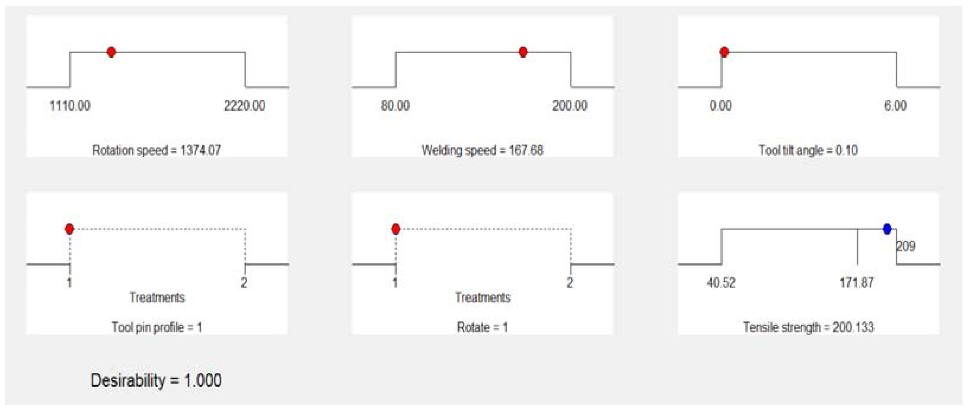
| Maximum tensile strength | MPa | 207.79 | |
| Variable Parameter | Unit | Result | Tensile Strength (Mpa) | % Difference | |
|---|---|---|---|---|---|
| Confirmed Experiment | VaNSAS | ||||
| Rotational speed | rpm | 2200 | 206.85 ± 0.886 | 207.79 | 1.93 |
| Welding speed | mm/min | 108.34 | |||
| Tool tilt | Deg | 1.23 | |||
| Pin profile | Hexagon | ||||
| Rotational direction | Clockwise | ||||
| Method | Tensile Strength (MPa) | % Diff |
|---|---|---|
| Base material specimen | 208.53 | - |
| Initial experiment | 171.87 | 17.58 |
| D-Optimal prediction | 200.13 | 4.02 |
| VaNSAS prediction | 207.79 | 0.35 |
| Confirmed experiment | 206.85 | 0.80 |
| Method | % Tensile Strength Difference of Method |
|---|---|
| Initial experiment vs. D-Optimal | 14.12 |
| Initial experiment vs. VaNSAS | 17.28 |
| Initial experiment vs. confirmed experiment | 16.91 |
| VaNSAS | 3.68 |
| D-Optimal vs. confirmed experiment | 3.24 |
| VaNSAS vs. confirmed experiment | 0.45 |
| Instances | Authors | Ultimate Tensile Strength/Tensile Strength (MPa) | |||
|---|---|---|---|---|---|
| D-Optimal/RSM | GA | DE | VaNSAS | ||
| 1 | Meengam and Sillapasa [28] | 120.7 | 123.55 | 124.82 | 125.11 |
| 2 | Jenarthanan et al. [71] | 105.47 | 106 | 107.63 | 108.02 |
| 3 | Tanmoy Medhi et al. [72] | 129.73 | 132.22 | 134.25 | 135.06 |
| 4 | Shanavas and Edwin raja dhas [33] | 202.58 | 204 | 206.86 | 206.54 |
| 5 | Ramanjaneyulu et al. [15] | 445 | 448.51 | 452.22 | 454.12 |
| 6 | Farzad et al. [73] | 535.5 | 536.24 | 538.62 | 540.08 |
| 7 | Masoud Ahmadnia et al. [74] | 187.35 | 210.53 | 211.24 | 212.54 |
| 8 | Ravi Sankar and Umamaheswarrao [75] | 184 | 186.35 | 187.39 | 189.32 |
| 9 | Hridya Nand Singh et al. [76] | 236 | 238.45 | 239.62 | 240.06 |
| 10 | Amit Goyal and Ramesh Kumar Garg [77] | 253.4 | 255.43 | 258.91 | 260.20 |
| 11 | JANNET et al. [78] | 288 | 288.54 | 290.78 | 290.98 |
| 12 | Kavitha et al. [79] | 211.48 | 211.95 | 212.97 | 213.08 |
| GA | DE | VaNSAS | |
|---|---|---|---|
| D-optimal | 0.002 | 0.002 | 0.002 |
| GA | 0.002 | 0.002 | |
| DE | 0.005 |
Publisher’s Note: MDPI stays neutral with regard to jurisdictional claims in published maps and institutional affiliations. |
© 2021 by the authors. Licensee MDPI, Basel, Switzerland. This article is an open access article distributed under the terms and conditions of the Creative Commons Attribution (CC BY) license (https://creativecommons.org/licenses/by/4.0/).
Share and Cite
Chainarong, S.; Srichok, T.; Pitakaso, R.; Sirirak, W.; Khonjun, S.; Akararungruangku, R. Variable Neighborhood Strategy Adaptive Search for Optimal Parameters of SSM-ADC 12 Aluminum Friction Stir Welding. Processes 2021, 9, 1805. https://doi.org/10.3390/pr9101805
Chainarong S, Srichok T, Pitakaso R, Sirirak W, Khonjun S, Akararungruangku R. Variable Neighborhood Strategy Adaptive Search for Optimal Parameters of SSM-ADC 12 Aluminum Friction Stir Welding. Processes. 2021; 9(10):1805. https://doi.org/10.3390/pr9101805
Chicago/Turabian StyleChainarong, Suppachai, Thanatkij Srichok, Rapeepan Pitakaso, Worapot Sirirak, Surajet Khonjun, and Raknoi Akararungruangku. 2021. "Variable Neighborhood Strategy Adaptive Search for Optimal Parameters of SSM-ADC 12 Aluminum Friction Stir Welding" Processes 9, no. 10: 1805. https://doi.org/10.3390/pr9101805
APA StyleChainarong, S., Srichok, T., Pitakaso, R., Sirirak, W., Khonjun, S., & Akararungruangku, R. (2021). Variable Neighborhood Strategy Adaptive Search for Optimal Parameters of SSM-ADC 12 Aluminum Friction Stir Welding. Processes, 9(10), 1805. https://doi.org/10.3390/pr9101805