
Handling Measurement Delay in Iterative Real-Time Optimization Methods


Abstract
:1. Introduction
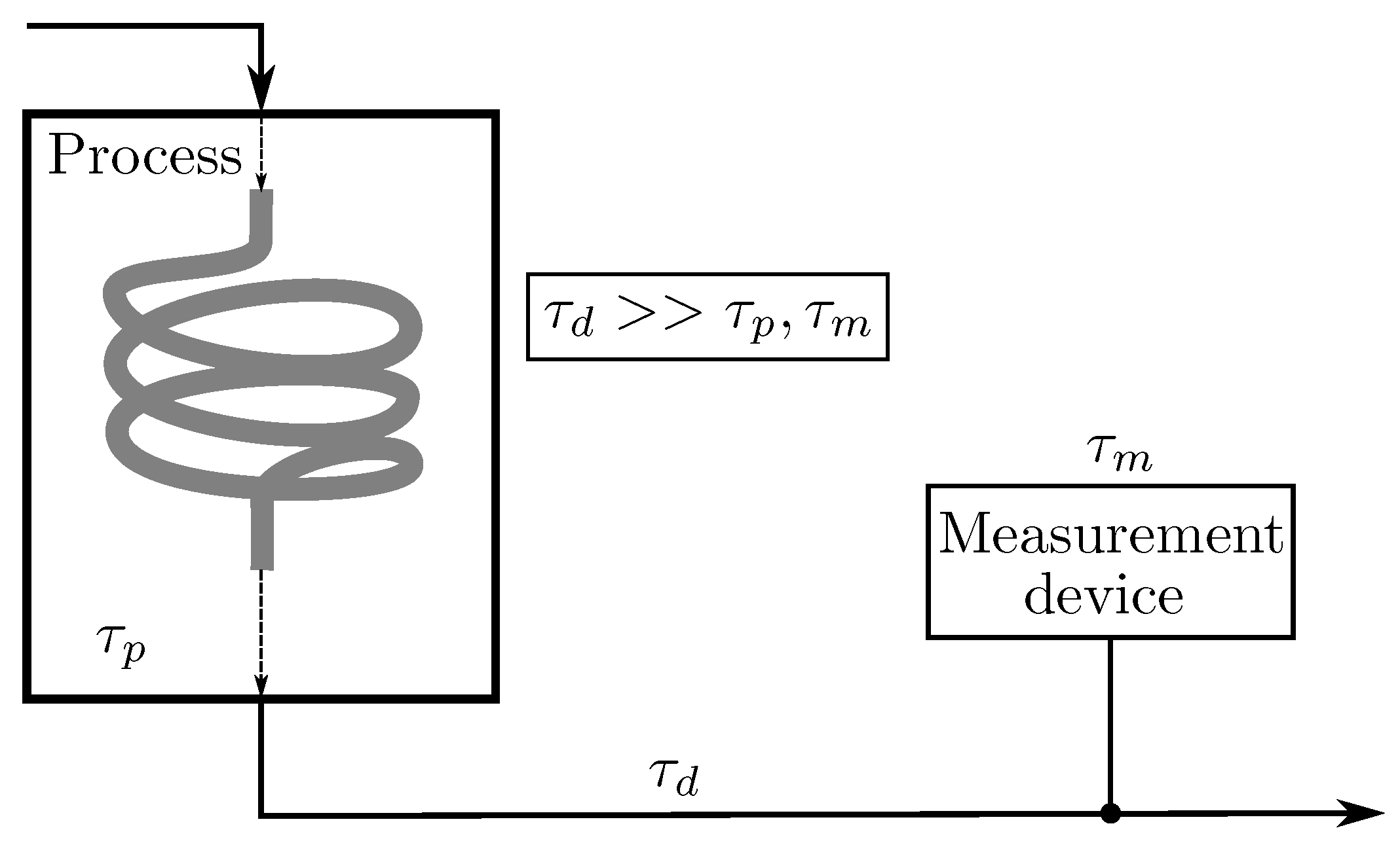
2. Preliminaries
2.1. Model
2.2. Modifier Adaptation
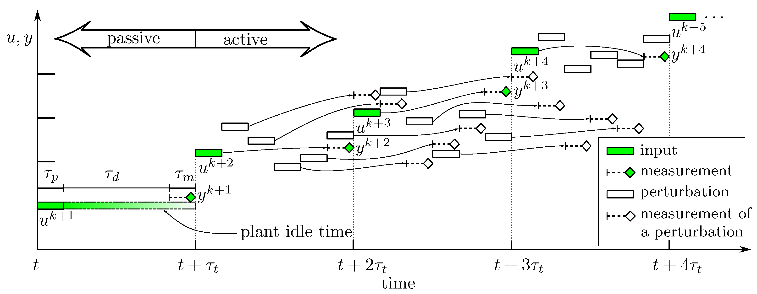
3. Active Perturbation Strategies
3.1. Active Perturbation around the Current Input (APCI)
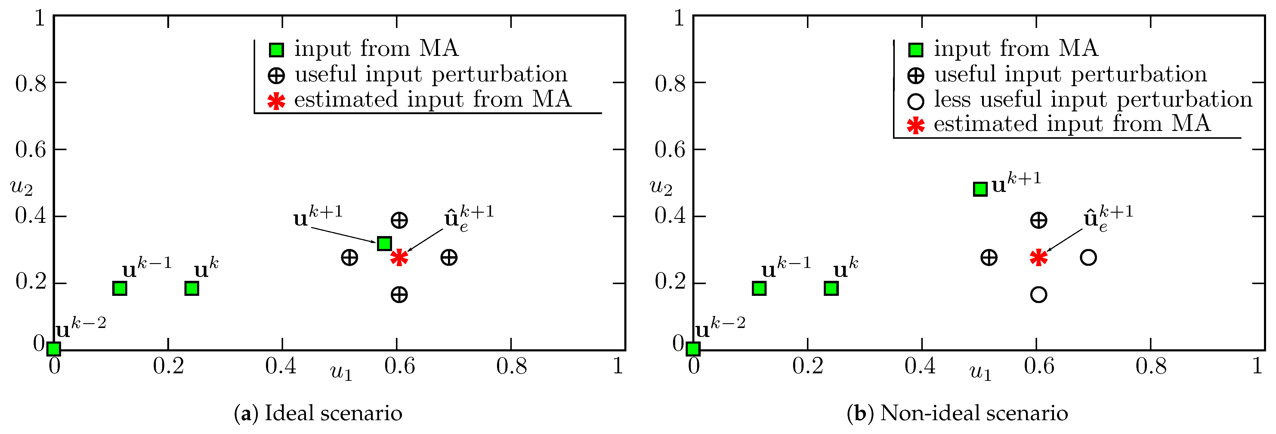
 represents the inputs from MA. Let be the input given to the plant in the kth iteration at time t. The plant reaches its steady-state at , and the steady-state measurements for are available at . During the waiting period, i.e., from to , additional perturbations represented by circles (◯) are performed around . Redundant probing is avoided by suppressing perturbation inputs that are closer than a threshold from one of the earlier inputs. For example, the perturbing input represented by is suppressed as it is in close vicinity to , and therefore, would be redundant. During the remaining waiting period, which is available due to suppressing of some perturbations, the plant is given the best known input to avoid a loss of performance. As the perturbing inputs are not computed optimally, not all of them provide useful information. For example, in Figure 3, only the perturbation inputs represented by are used by the QA scheme for computing the gradient at .
3.2. Active Perturbation around an Estimate of the Next Input (APENI)
4. Proactive Perturbation Scheme
- ➀
- perturbation input for gradient estimation using FD
- ➁
- perturbation input for gradient estimation using FD, also considered as an input () for MA problem formulation
- ➂
- perturbation input to gain additional information during the waiting period
- ➃
- perturbation input to gain additional information during the waiting period, also considered as an input () for MA problem formulation
- ➄
- input () computed by solving a MA problem (4) with plant gradients approximated using FD
- ➅
- perturbation input considered as an input () for MA problem formulation, to ensure a continuous flow of steady-state measurements every units of time
- ➆
- input () computed by solving MA problem with gradients approximated from past (at least ℓ) measurements
5. Williams–Otto Reactor Case Study
5.1. Process Description
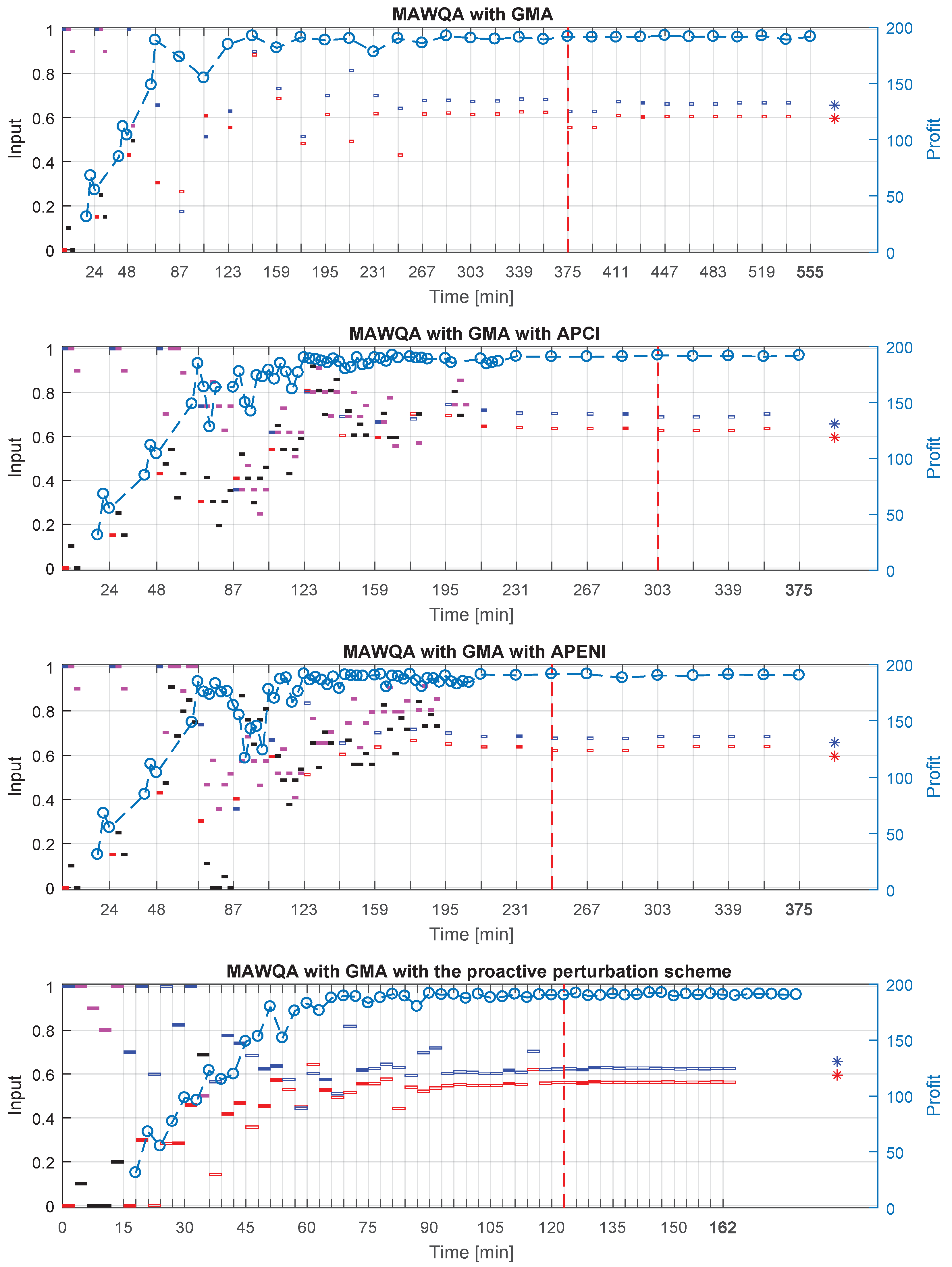
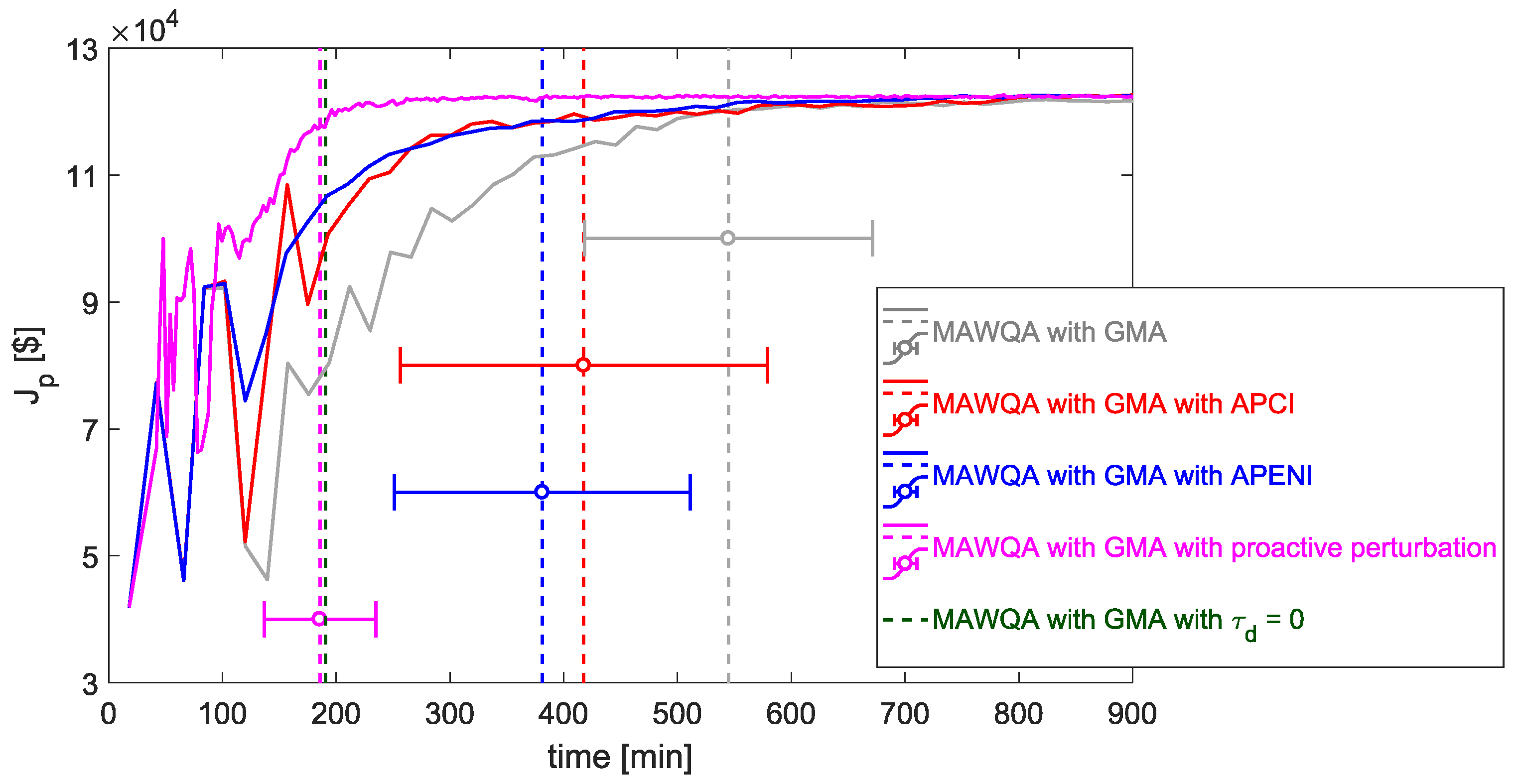
5.2. Simulation Results
 ) can be found on the right-side of the plot and the axis for the inputs (scaled) to the plant is on the left. Each vertical grid line in the plot represents the completion of an iteration, which includes all steps from giving input to a process to computing a new input by solving a modifier-adaptation problem. For MAWQA with GMA and MAWQA with GMA with active perturbation schemes APCI and APENI, after applying ([
  ,
,  ]) at , two input steps (perturbations [
  ,
,  ]) with a scaled step length are performed to compute the plant gradients using finite differences. Each input is applied to the plant until it reaches a steady-state, i.e., for . The steady-state plant measurement ( ) for each applied input are obtained after from applying an input. Upon computing the plant gradients using the steady-state plant measurements, the modifier adaptation problem in (4) is solved to compute the the input . As the condition for cardinality is not met, i.e., , additional perturbations ([ , ]) are performed after ([ , ]) to compute the plant gradients. Similar to the 0th iteration, the MA problem in (4) is solved in the iteration to compute . From here on, the cardinality condition is always satisfied. Therefore, QA is used for gradient approximation for all further iterations. In MAWQA with GMA, additional input perturbations are made only if the criticality-check criterion is not satisfied, for example in the iteration after applying to the plant., ]) to the plant, as and , two input perturbations ([ , ]) are performed to compute the plant gradients using finite differences. All necessary steady-state measurements for gradient correction, i.e., and two additional perturbations are available after 24 . During the waiting period, i.e., from 9 to 24 , additional input perturbations are performed to gain additional plant information. As the input perturbations when are considered as inputs from MA (according to the flowsheet in Figure 6), among the 5 additional perturbations, are renamed as . At 24 , steady-state measurements for and are available. Therefore, an MA problem is formulated and solved to compute the next input . For the next iteration, as and , FD is no more used for gradient approximation. However, there are not enough measurements for QA, i.e., , after applying . As , input perturbations and are added to smoothly switch from using FD for gradient approximation to QA. After , and a new steady-state measurement is always available every thereby overcoming and . From here on, a new iteration input is computed every taking into account the latest measurement information available.
6. Lithiation Process Case Study
6.1. Process Description
6.2. Simulation Results
7. Conclusions
Author Contributions
Funding
Conflicts of Interest
Symbols
| input variables | |
| number of input variables | |
| true process model | |
| nominal process model | |
| measured variables | |
| values of the measured variables estimated using a nominal process model | |
| number of measured variables | |
| number of constraint functions in the optimization problem | |
| true process optimum | |
| optimum computed using a nominal process model | |
| lower bound of the input variables | |
| upper bound of the input variables | |
| cost function in the optimization problem | |
| cost function computed using true process measurements | |
| cost function computed using estimated values of the measured variables | |
| cost function of the modifier adaptation problem in the kth iteration | |
| cost function of the optimization problem to estimate | |
| constraint functions of the optimization problem | |
| constraint functions evaluated using the true process measurements | |
| constraint functions evaluated using estimated values of the measured variables | |
| constraint functions of the modifier adaptation problem in the kth iteration | |
| constraint functions of the optimization problem to estimate | |
| ∇ | gradient operator |
| quadratic function | |
| parameters of the quadratic function | |
| ℓ | number of parameters in the quadratic function |
| set of all data points available until the kth iteration of MA | |
| selected data points for quadratic approximation in the kth iteration of MA | |
| anchor points in | |
| neighboring points in | |
| Δu | radius of the inner circle (tuning parameter) |
| Δ | step length for finite differences (tuning parameter) |
| minimum value for the inverse of the condition number (tuning parameter) | |
| inverse of the condition number in the kth iteration of MA | |
| input variables for the iteration computed by solving the MA problem in kth iteration | |
| estimated input variables for the iteration | |
| tuning parameter to scale the trust region (tuning parameter) | |
| cov | covariance operator |
| evaluation function to identify the convergence of MA to true process optimum | |
| accepted variance of for convergence (tuning parameter) | |
| best value of cost function computed using the plant measurements until the kth iteration of MA | |
| number of iterations the convergence criterion has to be satisfied (tuning parameter) | |
| time taken by the process to reach steady-state after a change of the inputs | |
| time required for the sample to reach (or to be transported to) the measurement device | |
| time required for the measurement device to analyze the sample | |
| total time to obtain steady-state measurements after a change in the input | |
| maximum possible number of input perturbations in the waiting period | |
| number of inputs given to the process, including the inputs whose measurements are not available | |
| number of inputs given to the process for whom the measurements are already available | |
| threshold to stop active perturbations (tuning parameter) | |
| threshold for unsuccessful iteration (tuning parameter) | |
| number of times an unsuccessful input can be probed (tuning parameter) |
Abbreviations
| RTO | Real-time optimization |
| SQP | Sequential quadratic programming |
| ISOPE | Integrated system optimization and parameter estimation |
| IGMO | Iterative gradient modification optimization |
| MA | Modifier adaptation |
| FD | Finite differences |
| QA | Quadratic approximation |
| DFO | Derivative free optimization |
| MAWQA | Modifier adaptation with quadratic approximation |
| APCI | Active perturbation around the current input |
| APENI | Active perturbation around an estimate of the next input |
| GMA | Guaranteed model adequacy |
| NMR | Nuclear magnetic resonance |
| ATEX | Atmosphere explosibles |
| IECEx | International electrotechnical commission explosive |
References
- Marchetti, A.G.; François, G.; Faulwasser, T.; Bonvin, D. Modifier Adaptation for Real-Time Optimization–Methods and Applications. Processes 2016, 4, 55. [Google Scholar] [CrossRef] [Green Version]
- Marlin, T.E.; Hrymak, A.N. Real-time operations optimization of continuous processes. In Chemical Process Control-V; AIChE Symposium Series; American Institute of Chemical Engineers: New York, NY, USA, 1997; Volume 93, pp. 156–164. [Google Scholar]
- Philip, E.; Murray, W.; Saunders, M.A.; Wright, M.H. User’s Guide for NPSOL 5.0: A Fortran Package for Nonlinear Programming; Technical Report SOL 86–6; Stanford University: Stanford, CA, USA, 2001. [Google Scholar]
- Gill, P.E.; Murray, W.; Saunders, M.A. SNOPT: An SQP Algorithm for Large-Scale Constrained Optimization. SIAM Rev. 2005, 47, 99–131. [Google Scholar] [CrossRef]
- Wächter, A.; Biegler, L.T. On the implementation of an interior-point filter line-search algorithm for large-scale nonlinear programming. Math. Program. 2006, 106, 25–57. [Google Scholar] [CrossRef]
- Kaustuv. IPSOL: An Interior Point Solver for Nonconvex Optimization Problems. Ph.D. Thesis, Stanford University, Stanford, CA, USA, 2009. [Google Scholar]
- Conn, A.R.; Scheinberg, K.; Vicente, L.N. Introduction to Derivative-Free Optimization; SIAM: Philadelphia, PA, USA, 2009. [Google Scholar]
- Rios, L.M.; Sahinidis, N.V. Derivative-free optimization: A review of algorithms and comparison of software implementations. J. Glob. Optim. 2013, 56, 1247–1293. [Google Scholar] [CrossRef] [Green Version]
- Jedrzejowicz, P. Current Trends in the Population-Based Optimization. In Proceedings of the 11th International Conference on Computational Collective Intelligence, Hendaye, France, 4–6 September 2019; Springer International Publishing: Cham, Switzerland, 2019; pp. 523–534. [Google Scholar]
- Wang, Z.; Qin, C.; Wan, B.; Song, W.W. A Comparative Study of Common Nature-Inspired Algorithms for Continuous Function Optimization. Entropy 2021, 23, 874. [Google Scholar] [CrossRef]
- Jang, S.S.; Joseph, B.; Mukai, H. On-line optimization of constrained multivariable chemical processes. AIChE J. 1987, 33, 26–35. [Google Scholar] [CrossRef]
- Chen, C.Y.; Joseph, B. On-line optimization using a two-phase approach: An application study. Ind. Eng. Chem. Res. 1987, 26, 1924–1930. [Google Scholar] [CrossRef]
- Roberts, P. An algorithm for steady-state system optimization and parameter estimation. Int. J. Syst. Sci. 1979, 10, 719–734. [Google Scholar] [CrossRef]
- Tatjewski, P. Iterative optimizing set-point control—The basic principle redesigned. IFAC Proc. Vol. 2002, 35, 49–54. [Google Scholar] [CrossRef] [Green Version]
- Gao, W.; Engell, S. Iterative set-point optimization of batch chromatography. Comput. Chem. Eng. 2005, 29, 1401–1409. [Google Scholar] [CrossRef]
- Marchetti, A.; Chachuat, B.; Bonvin, D. Modifier-adaptation methodology for real-time optimization. Ind. Eng. Chem. Res. 2009, 48, 6022–6033. [Google Scholar] [CrossRef] [Green Version]
- Gao, W.; Wenzel, S.; Engell, S. A reliable modifier-adaptation strategy for real-time optimization. Comput. Chem. Eng. 2016, 91, 318–328. [Google Scholar] [CrossRef] [Green Version]
- Roberts, P. Broyden derivative approximation in ISOPE optimising and optimal control algorithms. IFAC Proc. Vol. 2000, 33, 293–298. [Google Scholar] [CrossRef]
- Forbes, J.; Marlin, T.; MacGregor, J. Model adequacy requirements for optimizing plant operations. Comput. Chem. Eng. 1994, 18, 497–510. [Google Scholar] [CrossRef]
- Forbes, J.; Marlin, T. Design cost: A systematic approach to technology selection for model-based real-time optimization systems. Comput. Chem. Eng. 1996, 20, 717–734. [Google Scholar] [CrossRef]
- Bonvin, D.; Srinivasan, B. On the role of the necessary conditions of optimality in structuring dynamic real-time optimization schemes. Comput. Chem. Eng. 2013, 51, 172–180. [Google Scholar] [CrossRef] [Green Version]
- Faulwasser, T.; Bonvin, D. On the Use of Second-Order Modifiers for Real-Time Optimization. IFAC Proc. Vol. 2014, 47, 7622–7628. [Google Scholar] [CrossRef] [Green Version]
- Bunin, G.A.; François, G.; Bonvin, D. From Discrete Measurements to Bounded Gradient Estimates: A Look at Some Regularizing Structures. Ind. Eng. Chem. Res. 2013, 52, 12500–12513. [Google Scholar] [CrossRef] [Green Version]
- François, G.; Bonvin, D. Use of Convex Model Approximations for Real-Time Optimization via Modifier Adaptation. Ind. Eng. Chem. Res. 2013, 52, 11614–11625. [Google Scholar] [CrossRef] [Green Version]
- Ahmad, A.; Gao, W.; Engell, S. A study of model adaptation in iterative real-time optimization of processes with uncertainties. Comput. Chem. Eng. 2019, 122, 218–227. [Google Scholar] [CrossRef]
- Gottu Mukkula, A.R.; Engell, S. Guaranteed Model Adequacy for Modifier Adaptation with Quadratic Approximation. In Proceedings of the 2020 European Control Conference (ECC), St. Petersburg, Russia, 12–15 May 2020; pp. 1037–1042. [Google Scholar]
- Gao, W.; Hernández, R.; Engell, S. Real-time optimization of a novel hydroformylation process by using transient measurements in modifier adaptation. IFAC-PapersOnLine 2017, 50, 5731–5736. [Google Scholar] [CrossRef]
- Ferreira, T.D.A.; François, G.; Marchetti, A.G.; Bonvin, D. Use of Transient Measurements for Static Real-Time Optimization. IFAC-PapersOnLine 2017, 50, 5737–5742. [Google Scholar] [CrossRef]
- Rodríguez-Blanco, T.; Sarabia, D.; Pitarch, J.; de Prada, C. Modifier Adaptation methodology based on transient and static measurements for RTO to cope with structural uncertainty. Comput. Chem. Eng. 2017, 106, 480–500. [Google Scholar] [CrossRef]
- Cadavid, J.; Hernández, R.; Engell, S. Speed-up of Iterative Real-Time Optimization by Estimating the Steady States in the Transient Phase using Nonlinear System Identification. IFAC-PapersOnLine 2017, 50, 11269–11274. [Google Scholar] [CrossRef]
- Krishnamoorthy, D.; Jahanshahi, E.; Skogestad, S. Feedback Real-Time Optimization Strategy Using a Novel Steady-state Gradient Estimate and Transient Measurements. Ind. Eng. Chem. Res. 2018, 58, 207–216. [Google Scholar] [CrossRef]
- Gottu Mukkula, A.R.; Wenzel, S.; Engell, S. Active Perturbation in Modifier Adaptation for Real Time Optimization to Cope with Measurement Delays. IFAC-PapersOnLine 2018, 51, 124–129. [Google Scholar] [CrossRef]
- Gottu Mukkula, A.R.; Wenzel, S.; Engell, S. Active Perturbations Around Estimated Future Inputs in Modifier Adaptation to Cope with Measurement Delays. IFAC-PapersOnLine 2018, 51, 839–844. [Google Scholar] [CrossRef]
- Brdyś, M.; Tatjewski, P. An Algorithm for Steady-State Optimizing Dual Control of Uncertain Plants. IFAC Proc. Vol. 1994, 27, 215–220. [Google Scholar] [CrossRef]
- Gao, W.; Wenzel, S.; Engell, S. Modifier adaptation with quadratic approximation in iterative optimizing control. In Proceedings of the 2015 IEEE European Control Conference (ECC), Linz, Austria, 15–17 July 2015; pp. 2527–2532. [Google Scholar]
- Wenzel, S.; Yfantis, V.; Gao, W. Comparison of regression data selection strategies for quadratic approximation in RTO. Comput. Aided Chem. Eng. 2017, 40, 1711–1716. [Google Scholar]
- Gao, W.; Wenzel, S.; Engell, S. Integration of gradient adaptation and quadratic approximation in real-time optimization. In Proceedings of the 2015 34th Chinese Control Conference (CCC), Hangzhou, China, 28–30 July 2015; pp. 2780–2785. [Google Scholar]
- Gottu Mukkula, A.R.; Ahmad, A.; Engell, S. Start-up and Shut-down Conditions for Iterative Real-Time Optimization Methods. In Proceedings of the 2019 Sixth Indian Control Conference (ICC), Hyderabad, India, 18–20 December 2019; pp. 158–163. [Google Scholar]
- Williams, T.J.; Otto, R.E. A generalized chemical processing model for the investigation of computer control. Trans. Am. Inst. Electr. Eng. Part I Commun. Electron. 1960, 79, 458–473. [Google Scholar] [CrossRef]
- Friedman, M. The Use of Ranks to Avoid the Assumption of Normality Implicit in the Analysis of Variance. J. Am. Stat. Assoc. 1937, 32, 675–701. [Google Scholar] [CrossRef]
- Gottu Mukkula, A.; Kern, S.; Salge, M.; Holtkamp, M.; Guhl, S.; Fleicher, C.; Meyer, K.; Remelhe, M.; Maiwald, M.; Engell, S. An Application of Modifier Adaptation with Quadratic Approximation on a Pilot Scale Plant in Industrial Environment. IFAC-PapersOnLine 2020, 53, 11773–11779. [Google Scholar] [CrossRef]
- Bieringer, T.; Buchholz, S.; Kockmann, N. Future production concepts in the chemical industry: Modular–small-scale–continuous. Chem. Eng. Technol. 2013, 36, 900–910. [Google Scholar] [CrossRef]
- Kern, S.; Wander, L.; Meyer, K.; Guhl, S.; Gottu Mukkula, A.R.; Holtkamp, M.; Salge, M.; Fleischer, C.; Weber, N.; King, R.; et al. Flexible automation with compact NMR spectroscopy for continuous production of pharmaceuticals. Anal. Bioanal. Chem. 2019, 411, 3037–3046. [Google Scholar] [CrossRef] [PubMed] [Green Version]


| No. | Parameter | Williams–Otto | Lithiation Reaction |
|---|---|---|---|
| 1. | trust-region scaling | 3 | 3 |
| 2. | radius of inner circle | 0.1 | 0.125 |
| 3. | step length for finite differences | 0.1 | 0.2 |
| 4. | conditionality limit | 0.2 | 0.25 |
| 5. | threshold to stop active perturbations | 0.05 | 0.1 |
| 6. | threshold for unsuccessful iteration | 0.005 | 0.005 |
| 7. | number of times an unsuccessful input | 3 | 3 |
| is probed | |||
| 8. | number of inputs looked at for | 5 | 5 |
| convergence | |||
| 9. | accepted variance of J | − | |
| for convergence |
| Marker | Description |
|---|---|
| [ , ] | successful-iteration input () |
[  , ,  ] ] | unsuccessful-iteration input () |
| [ , ] | perturbation input () |
| | value of the plant profit function |
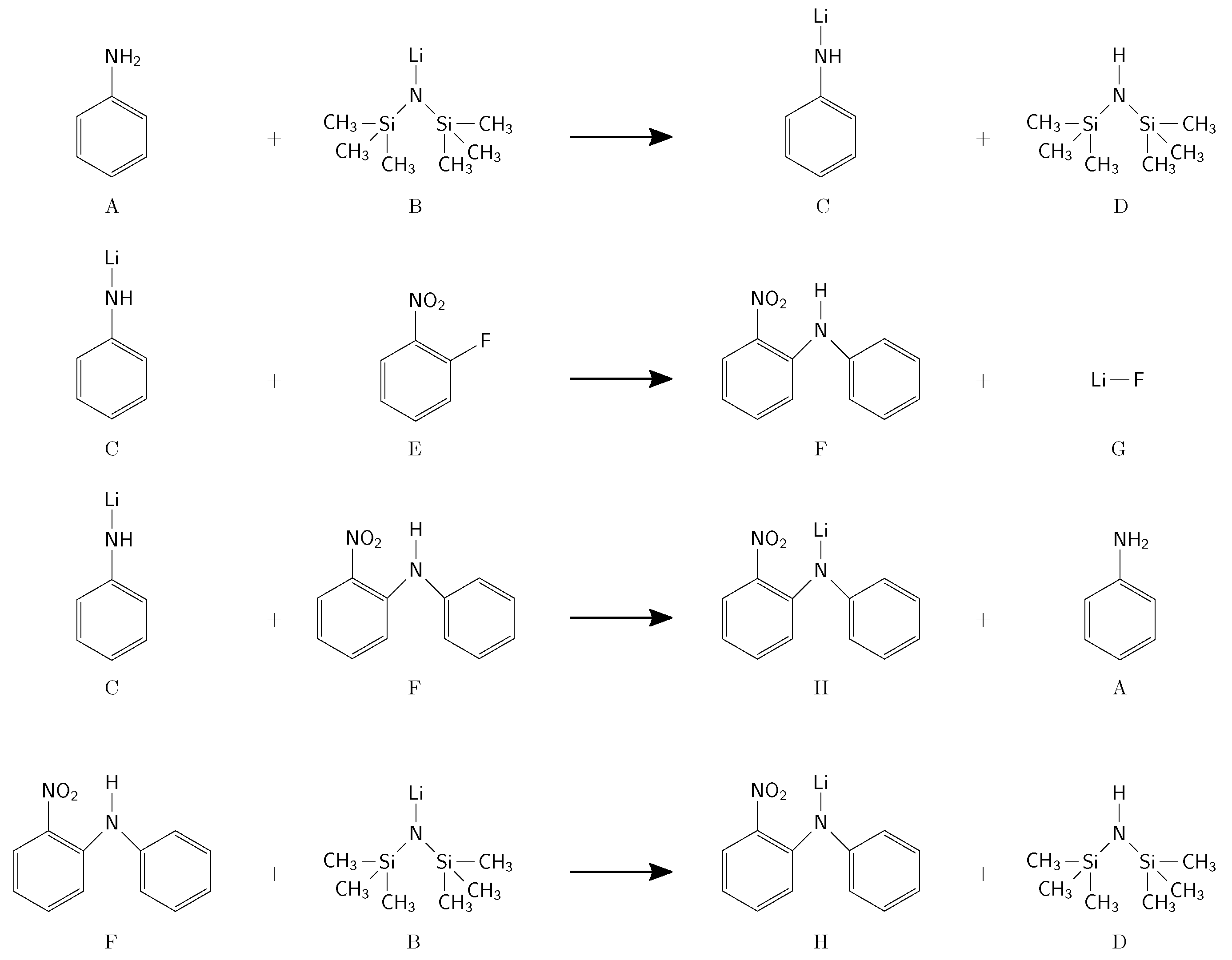
| Label | Chemical Name (Abbreviation) | Role |
|---|---|---|
| A | Aniline (An) | reactant |
| B | Lithium bis(trimethylsilyl)amide (Li-HMDS) | reactant |
| C | Lithium phenylazanide (Li-An) | intermediate |
| D | Hexamethyldisilazane (HMDS) | by-product |
| E | 1-Fluoro-2-nitrobenzene (FNB) | reactant |
| F | 2-Nitrodiphenylamine (NDPA) | intermediate |
| G | Lithium fluoride (LiF) | by-product |
| H | Lithium 2-Nitrodiphenylamine (Li-NDPA) | product |
| Tetrahydrofuran (THF) | solvent |
| Parameter | Value | Parameter | Value |
|---|---|---|---|
| / | |||
| E | / | ||
| / | / | ||
| /() | |||
| 900 / | R | /() |
Publisher’s Note: MDPI stays neutral with regard to jurisdictional claims in published maps and institutional affiliations. |
© 2021 by the authors. Licensee MDPI, Basel, Switzerland. This article is an open access article distributed under the terms and conditions of the Creative Commons Attribution (CC BY) license (https://creativecommons.org/licenses/by/4.0/).
Share and Cite
Gottu Mukkula, A.R.; Engell, S. Handling Measurement Delay in Iterative Real-Time Optimization Methods. Processes 2021, 9, 1800. https://doi.org/10.3390/pr9101800
Gottu Mukkula AR, Engell S. Handling Measurement Delay in Iterative Real-Time Optimization Methods. Processes. 2021; 9(10):1800. https://doi.org/10.3390/pr9101800
Chicago/Turabian StyleGottu Mukkula, Anwesh Reddy, and Sebastian Engell. 2021. "Handling Measurement Delay in Iterative Real-Time Optimization Methods" Processes 9, no. 10: 1800. https://doi.org/10.3390/pr9101800
APA StyleGottu Mukkula, A. R., & Engell, S. (2021). Handling Measurement Delay in Iterative Real-Time Optimization Methods. Processes, 9(10), 1800. https://doi.org/10.3390/pr9101800