1. Introduction
Owing to the advantages of good gas–solid mixing characteristics, gas–solid contacting behaviors, heat transfer properties, and reaction characteristics, the circulating fluidized bed has been widely used in chemical process, energy-related processes, mineral processes, and so on.
A typical CFB consists of the riser, cyclones, the downcomer, and the valve, as shown in
Figure 1. In the riser, gas from the bottom carries particles from the downcomer in an upward direction. In the top of the riser, through gas–solids separators such as cyclones, particles are separated from the gas downward back to the downcomer, while gas flows out of the system from the top of the cyclones. In industrial applications, the riser is usually used as the main reactor, while the downcomer is usually used as a storage device to adjust particles, a heat exchanger, a catalyst regenerator, or simply as a standpipe to maintain circulation of solids.
To optimize the products of the reactor, both excellent design and reasonable operation of the CFB, which are closely related to the gas–solids distribution, solids back-mixing, and residence time distribution, are critical. Extensive experiment and simulation studies focused on the gas–solids flow characteristics of CFB and found plenty of useful results such as solids holdup distribution, velocity distribution, solids back-mixing, and effects of both geometry and operating conditions [
1,
2,
3,
4].
Because of the high cost of experimental research, a large number of researchers have studied gas–solids flow in a circulating fluidized bed by numerical simulation [
5,
6,
7,
8].
To minimize computational requirements, 2D simulations for the riser were conducted in the literature. In 2D simulation, the cylindrical column is simplified as an infinite volume comprised between two planes. However, 2D simulation could not predict the asymmetric entry of particles, and usually could not properly reflect the wall effect [
9]. Milinkumar [
10] compared three different inlet boundary conditions in the 2D domain, and found that it is challenging to select proper boundary conditions in 2D simulations of the riser. Therefore, 3D simulation of the riser is necessary to investigate more realistic hydrodynamics in the riser.
Owing to the limitation of the computing capacity, some previous simulations simplified the riser as a vertical pipe without considering the structure of the entrance and exit, setting up one inlet in the bottom of the riser as both the gas and solid inlet [
11]. Besides riser-simplified simulation, some researchers regarded the riser with the structure of the entrance and exit as the simulation object [
12]. The gas inlet is in the bottom of the riser and the solids inlet is from the side feeding pipe. The effects of different exit structures such as type C, type T, and type L could also be studied by this method [
13].
With the development of the model and computing capacity, more and more investigators conducted full-loop simulation of the CFB system [
14,
15,
16,
17,
18,
19,
20,
21,
22], which treats the CFB as a whole dynamic system. Chu et al. [
14] conducted a 3D full-loop simulation for CFB by means of the combined continuum and discrete method. The results were in good agreement with the experiment data. Zhang et al. [
15] applied EMMS drag correction on the full-loop simulation of a semi-industry scale CFB. The flow regime, especially choking and continuous transitions, was captured by simulation. Guan et al. [
16] conducted a full-loop simulation of a CFB including the riser, bubbling bed, pot-seal, and cyclone. From the results, they found a strong relationship between the solids flow pattern in the bubbling bed in the return system and superficial gas velocity in the riser. Wang et al. [
17] studied the effects of cyclone arrangements on the gas–solids flow dynamics in the 3D full-loop CFB and found that solids inventory is different in different cyclones. Furthermore, the solids inventory in cyclones in the axial symmetry arrangement was more uniform than that in the central symmetry arrangement. Nikolopoulos et al. [
18] simulated a CFB carbonator by the EMMS drag model with a proper friction model, successfully predicting pulsing behavior in the loop-seal.
The CFB is a system such as the one shown in
Figure 1. Without considering the model accuracy and computing cost, it is better to adopt full-loop simulation to obtain comprehensive information of the system. However, sometimes we need to compromise to maintain the balance between simulation accuracy and efficiency. It is critical to find whether riser-simplified simulation and riser-only simulation predict reliable results and how the results predicted by these methods differ from those predicted by full-loop simulation. There is limited work about the comparison of riser-simplified, riser-only, and full-loop simulation. Li [
18] compared riser-only and full-loop simulation, focusing on the role that mean solids circulation rates played on both simulations, and concluded that the mean solids circulation rate was critical in both riser-only and full-loop simulations. In riser-only simulation, the mean solids circulation rate is needed for specifying the solids inlet boundary condition. In full-loop simulation, the mean solids circulation rate is a parameter to be predicted. He found that the riser-only simulation with both constant and variable solids velocity at the inlet can predict steady flow in the riser, while full-loop simulation was more promising, but challenging because of the limitation of model and computer power.
This paper conducted riser-simplified, riser-only, and full-loop simulation for a circulating fluidized bed. The hydrodynamics were obtained from different methods. The pressure balance, solids holdup, solids vectors, and instantaneous characteristics in the CFB in different methods are compared in detail. The advantages and disadvantages of different methods are discussed to find the scope of application of riser-simplified, riser-only, and full-loop simulation.
2. Methods
Cases of riser-simplified, riser-only, and full-loop simulation are set up with the same models. The Eulerian–Eulerian model, together with the kinetic theory of granular flow (KTGF), was used to simulate the gas–solids flow in CFB in the present work. The gidaspow drag model [
23] was used to predict the momentum transfer between the gas and solid phase. The governing equations for gas–solids flow were shown in previous work [
6].
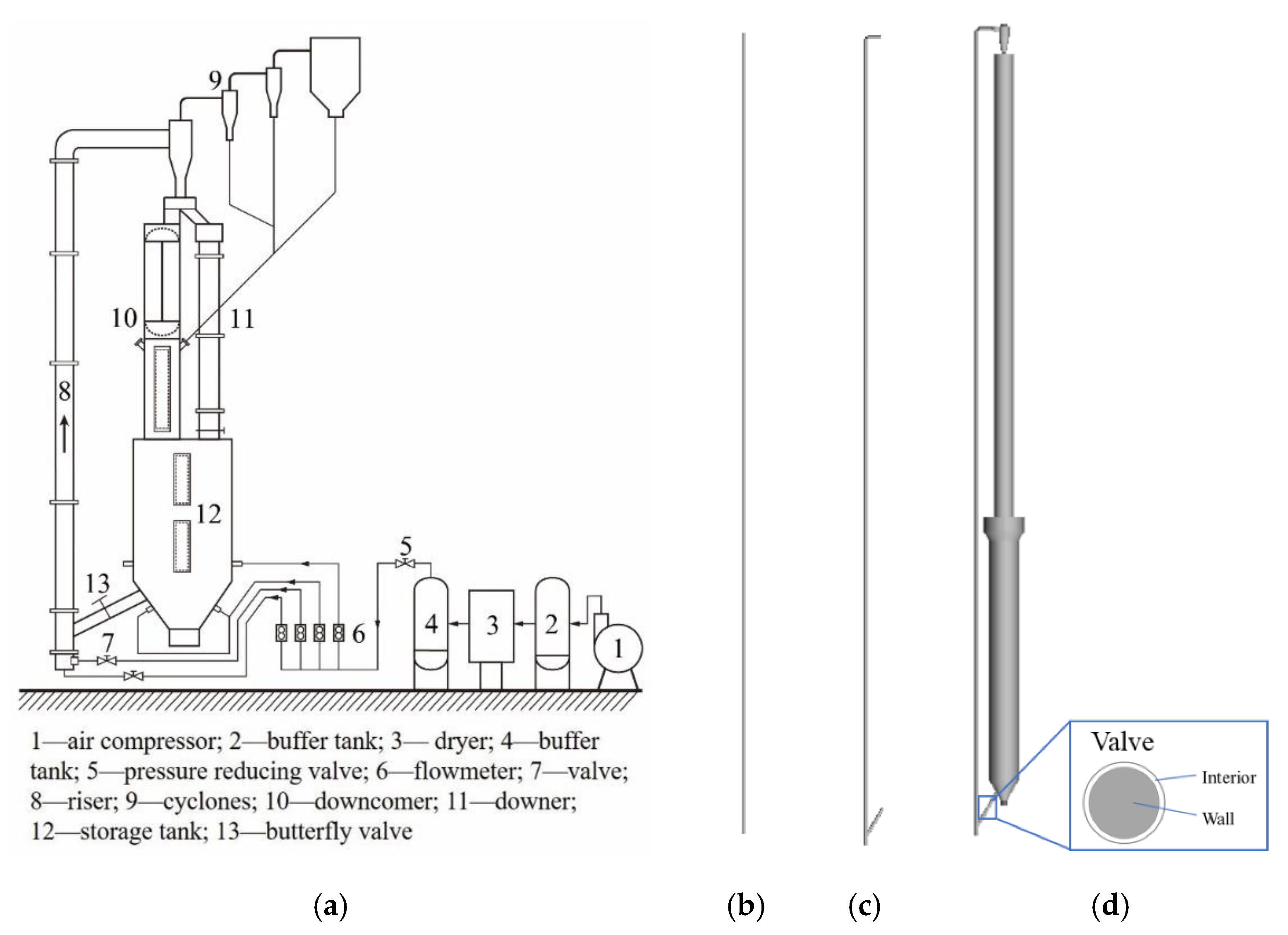
A pilot CFB shown in
Figure 2a was simulated by different methods. The CFB mainly consists of a riser, a downcomer, a storage tank, cyclones, and a feed pipe with a butterfly valve. The riser is at a height of 18 m and an inner diameter of 80 mm. The downcomer is at a height of 8 m and a diameter of 450 mm. The storage tank is at a height of 6 m and is 660 mm in diameter. The pressure transducer (Skysen, Beijing, China) and optical fiber densimeter (Institute of process engineering, Chinese Academy of Sciences, Beijing, China) were used to measure the hydrodynamics. The particles stored in the storage tank flowed into the inclined feed pipe. Because of the obstacle of the butterfly in the feed pipe, solids circulating rates were controlled by adjusting the opening degree of the valve. In the downstream of the valve, particles flowed into the bottom of the riser and were carried upward by the air from a compressor (Hitachi, Ltd., Tokyo, Japan). The gas–solids mixture in the top of the riser flowed into the cyclone, and particles were separated from the mixture back to the storage tank. To measure the solids circulation rate, the top of the downcomer was divided vertically into two parts with the same volume. Two flap valves were used in the top and bottom of the measuring part. At first, the top valve was opened and the bottom valve was closed. Particles flowed into the measuring part and accumulated. The solids circulating rate was calculated as
where
is the volume of particles in the measure part,
is the particle bulk density,
is the area of the cross section of the measure part, and
is the measuring period.
The simulation objects are shown in
Figure 2b–d. In the riser simulation, the return system is not included in the simulation object. To obtain a more reasonable result, the boundary condition of the solid inlet of the riser should be set up considering the effects of the return system. However, in the current riser simulation, the boundary condition of the solid inlet is usually set up as velocity–inlet with a certain volume fraction. There is little discussion about how to determine the value of the volume fraction, which is usually determined based on experience nowadays. In this work, the solid volume fraction is 0.25, which will be validated in
Section 3.1. In the riser-simplified simulation, the gas and solid inlet is defined in the central bottom of the riser with a solid volume fraction of 0.25. The outlet of the riser is a pressure-outlet. In the riser-only simulation, the gas inlet is in the bottom of the riser, and the solid inlet is in the inclined feed pipe with the same solid volume fraction and velocity as in the riser-simplified simulation. In the full-loop simulation, the inlet and the outlet of the riser are part of the system. There is no need to set up boundary conditions for them. In the initialization of the full-loop simulation, particles were patched at a height of 4 m, the same as in the experiment, in the storage tank. The inlet of the gas phase was a velocity inlet at the bottom of the riser. The outlet of the gas and solids was at the top of the cyclone as a pressure outflow. For the particles flow out of the outlet of cyclone, user-defined functions (UDFs) were used to let these particles flow back to the storage tank to maintain the material balance. Generally, two kinds of valves were used for controlling the solids flux. One is a non-mechanical valve, such as an L-valve, which controls Gs by adjusting aeration rates [
15]; the other one is a mechanical valve, such as the butterfly valve in the present work, which controls Gs by the opening degree of the valve. The former mainly changes the carrying capacity, while the latter mainly changes the circulation area. As for the mechanism valve, the flow area of the fluid is different for different opening degrees. Therefore, in this simulation, the valve opening was adjusted by changing the area through which fluid could flow. Such a flow area was set as the interior boundary condition, while the area through which fluid could not flow was set as the wall boundary condition, as shown in
Figure 2d. The material properties of both air and particles as well as operating conditions are shown in
Table 1, according to the experiment.
Simulations were conducted by Fluent 6.3 (ANSYS®, Pittsburgh, PA, USA). The governing equations were solved by a pressure-based approach. The momentum equations were solved in a second-order upwind scheme. The volume fraction of gas or solids was solved by a QUICK scheme. The phase-coupled SIMPLE algorithm was used to solve pressure–velocity coupling. A time step of 1 × 10⁻³ s was used for this study. The simulations ran for 60 s and the last 20 s were calculated for time-averaged computational results.
3. Results and Discussion
3.1. Validation
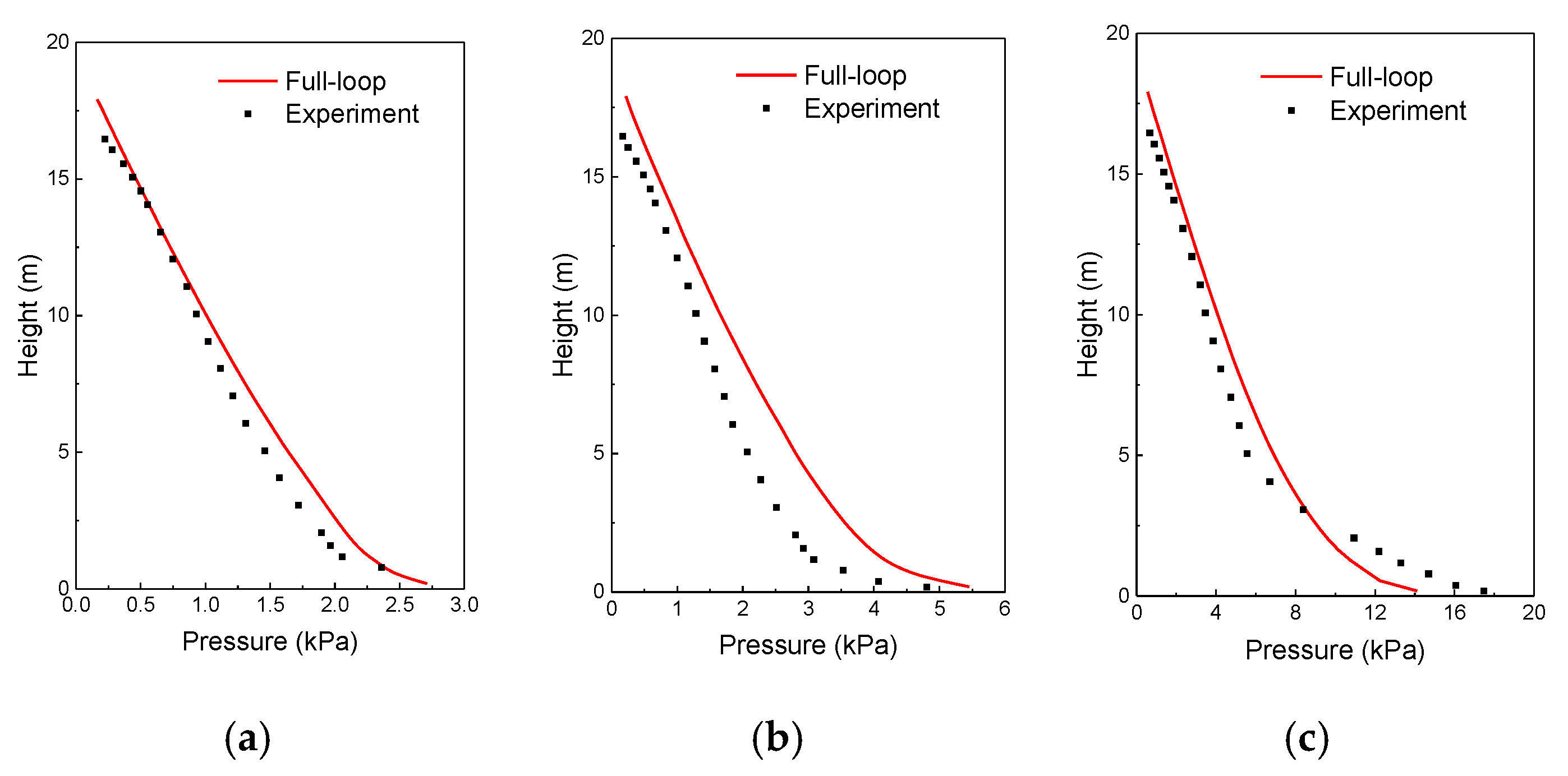
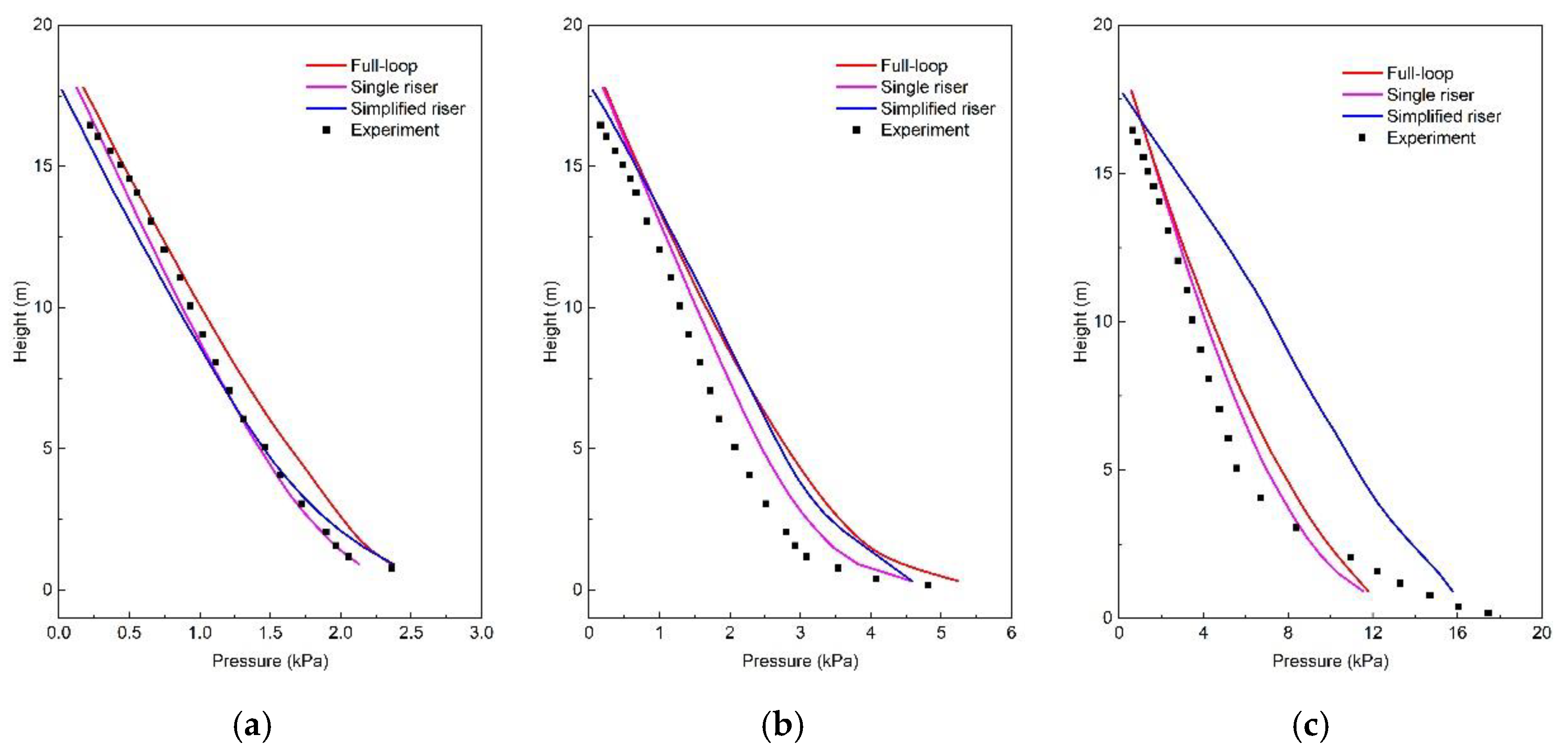
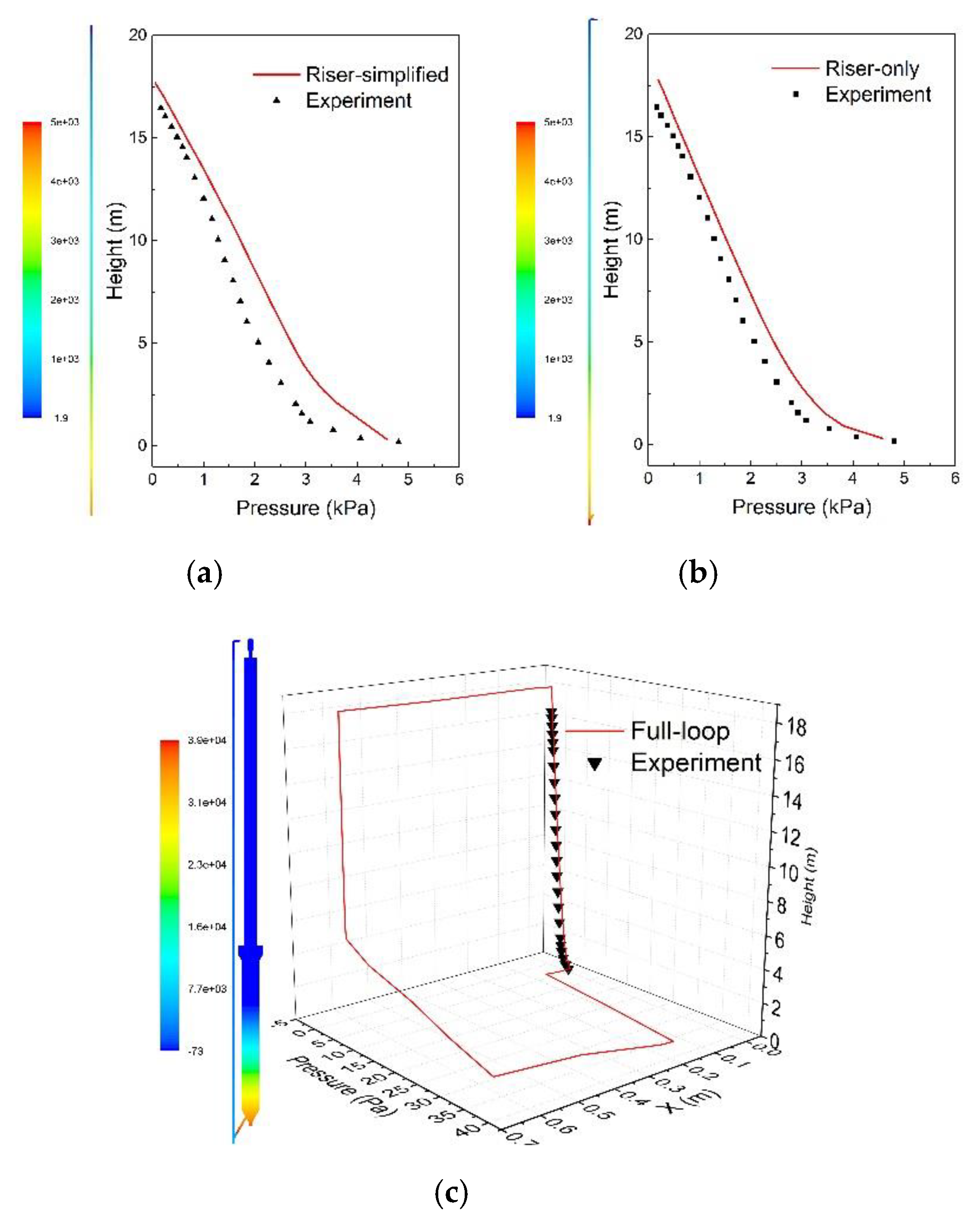
Figure 3 presents the time-averaged axial pressure profiles of the riser in the full-loop simulation and experiment. The pressure at the bottom of the riser is larger than that at the top, which pushes the gas and solids flow upward along riser. Pressure distributions in simulation agree well with that of the experiment in all operation conditions. The predicted pressure drop in the bottom of the riser was lower than the experimental data, which is possibly due to the fact that the Gidaspow drag model underestimated the solids volume fraction at the bottom of the riser.
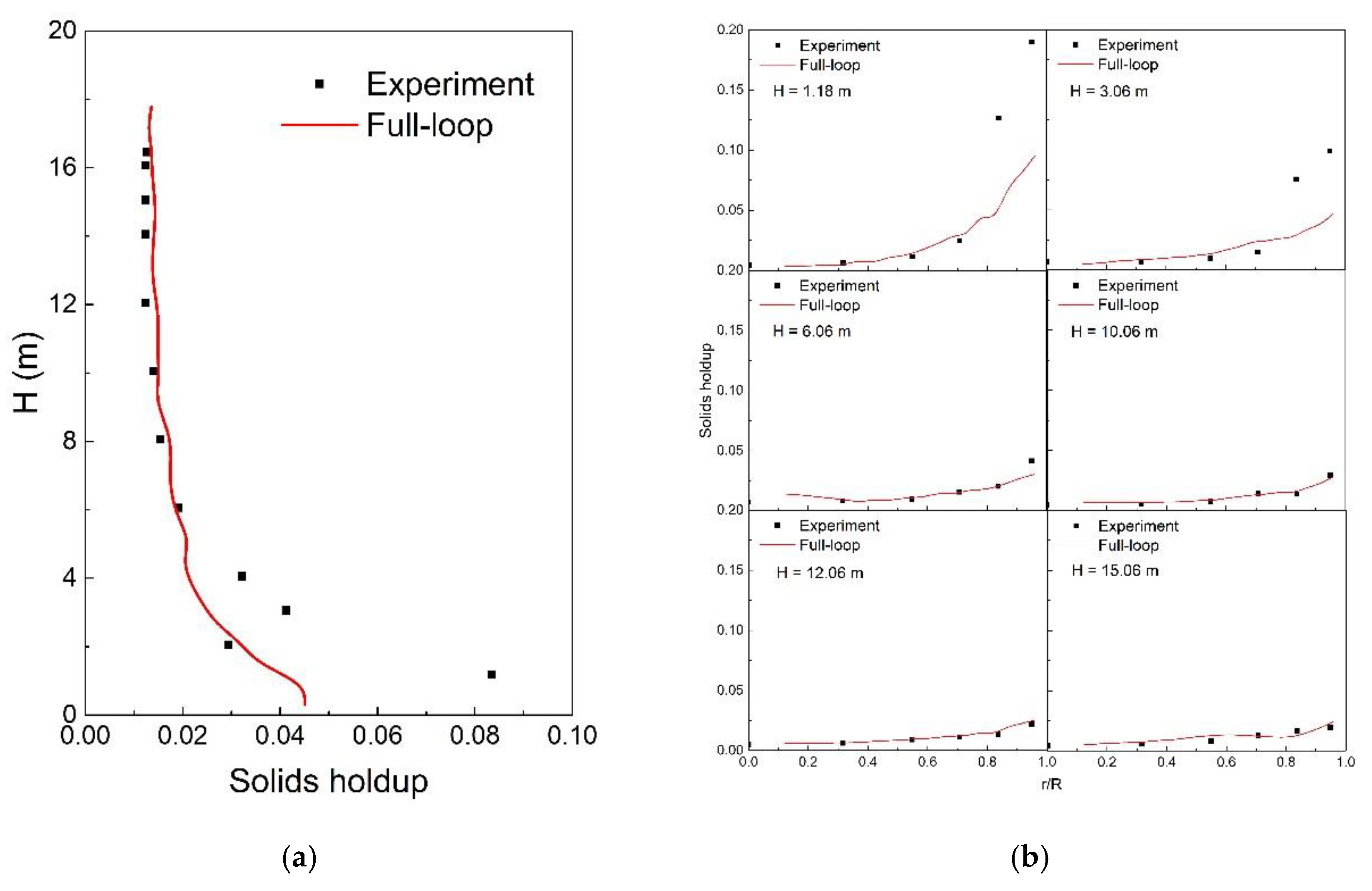
Figure 4 shows the comparison of time-averaged solids holdup profiles of the riser in the full-loop simulation and experiment. The solids holdup is higher at the bottom and lower at the top of the riser in the axial direction, which is consistent with pressure distribution. In the radial direction, though the solids holdup near the wall region is higher than that in the central region compared with experiment data, the full-loop simulation predicts well in both the axial and radial direction in the riser.
3.2. Comparison of Pressure Distribution in CFB between Different Methods
Figure 5 shows the comparison of pressure distribution in CFB between different simulations. The pressure in the simplified riser is reasonable at lower Gs, but quite different from that in the other two at Gs = 300 kg m
−2 s
−1. A possible reason is that the effects of the entrance and exit of the riser are critical in higher solids circulating rates. With the simplified entrance and exit, the riser-simplified simulation is not able to predict accurate results in high solids circulating rates. For the other two simulation methods, there is only a slight difference in the results, usually in the lower region of the riser, possibly because of the different inlet boundary condition of the riser.
Through the riser-simplified and riser-only simulation, we can only get the pressure drop in the riser, while with the full-loop simulation, we can get the pressure balance in whole system, as shown in
Figure 6. The CFB system consists of the riser, cyclones, the downcomer, the storage rank and the feed pipe with the valve. The back pressure of the solids in the storage tank provides a driving force to push the particles circulating in the loop. The pressure drops of other parts such as the riser, the valve, and the cyclone are the resistance of the system. In a stable CFB, the driving force is equal to the resistance, as presented in Equation (2).
where
is the pressure drop of the particles in the downcomer and storage tank,
is the pressure drop in the riser,
is the pressure drop of the cyclones, and
is the pressure drop of the feed pipe including the valve.
In the riser, the pressure decreases in the axial direction, while the pressure drop in the horizontal pipe from the riser exit to the cyclone is small. The pressure drops in the downcomer and upper zone in the storage tank are also limited because of the low solids holdup. At the bottom of storage tank, the pressure is very high because of the many particles stored in the storage tank. The pressure in the tank is high enough to push particles circulating in the system and to prevent gas leakage. Further, there is a sharp pressure drop in the valve, as shown in
Figure 6c.
In the design of a CFB, it is critical not only to focus on the pressure drop in the riser reactor, but also to consider the pressure balance of the CFB system to maintain a stable operation. In addition, some operation factors in the particle return system such as storage height and valve opening are critical. Only through the full-loop simulation can we study the effects of the return system.
3.3. Effects of Different Methods on Solids Holdup of the Riser
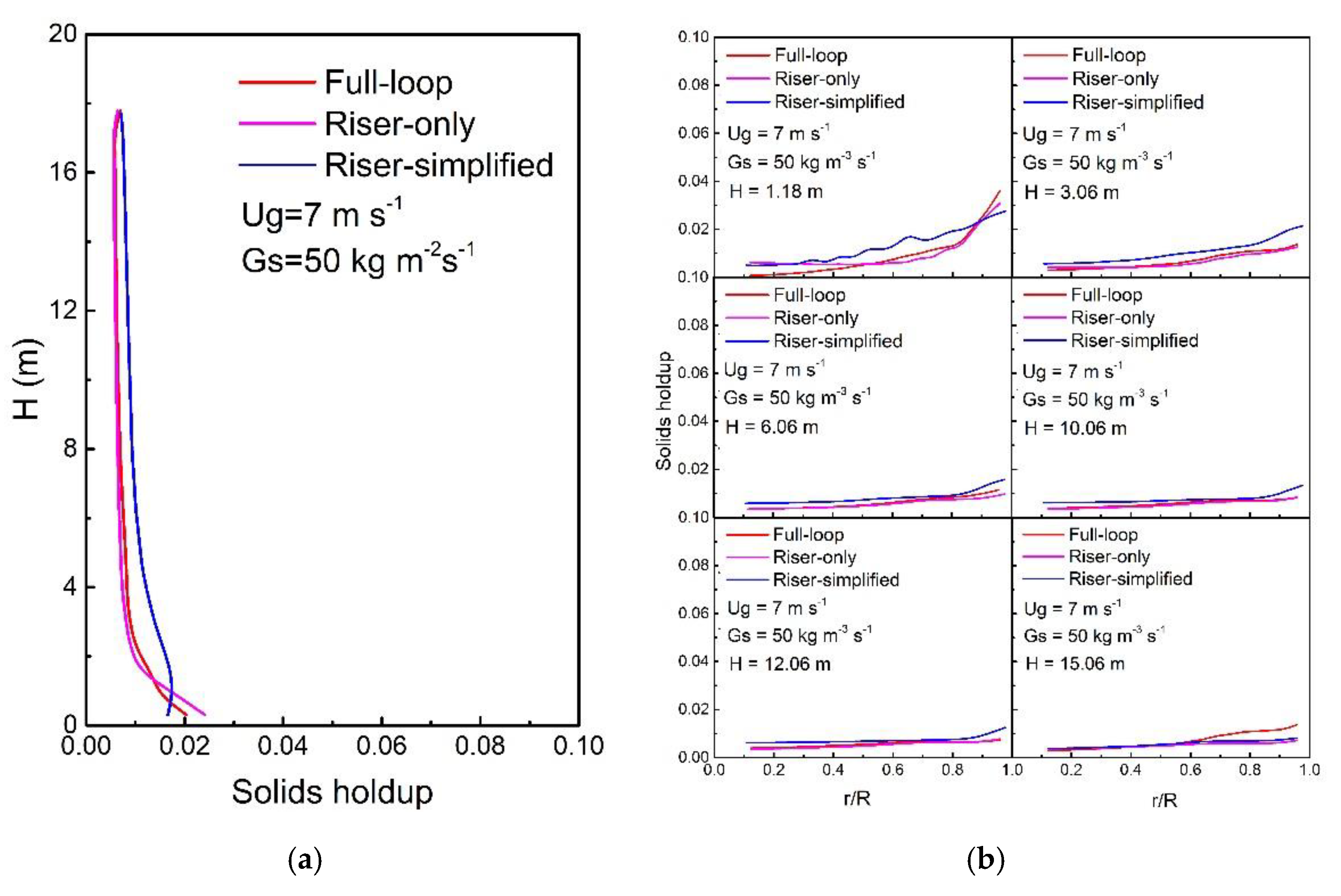
Figure 7 presents the comparison of solids holdup distribution in CFB between different methods in U
g = 7 m s
−1, Gs = 50 kg m
−2 s
−1. Solids holdup in the axial direction of the riser in the riser-simplified simulation is higher than that in the other two cases, while there is little difference between riser-only simulation and full-loop simulation. As for solids holdup in the radial direction, the solids holdup in riser-simplified simulation is also different from that of the other two methods. According to
Figure 7, the trends in both the axial and radial direction in low Gs are roughly similar.
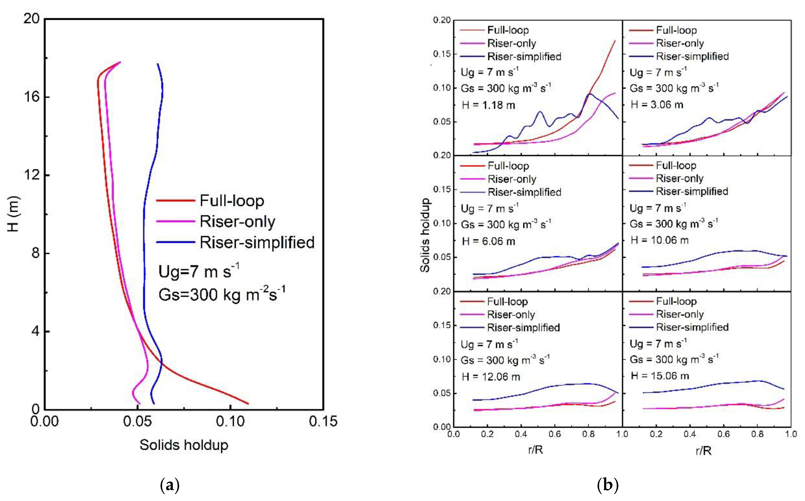
In higher Gs, such as 300 kg m
−2 s
−1 presented in
Figure 8, these methods predict different solids holdup distribution. The results of riser-simplified simulation deviate largely from those of the other two methods, as it could not accurately predict the gas–solid flow in the entrance and exit. For the other two methods, when Gs = 50 kg m
−2 s
−1, there is little difference among these methods. When it comes to Gs = 300 kg m
−2 s
−1, in the axial direction, the solids holdup at the bottom of the riser is lower than at the upper region predicted by the riser-only simulation, while the solids holdup at the bottom of the riser is higher than at the upper region predicted by the full-loop simulation. As a result, the fully-developed region in the riser-only simulation is longer than that in the full-loop simulation.
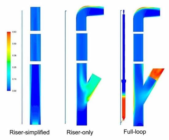
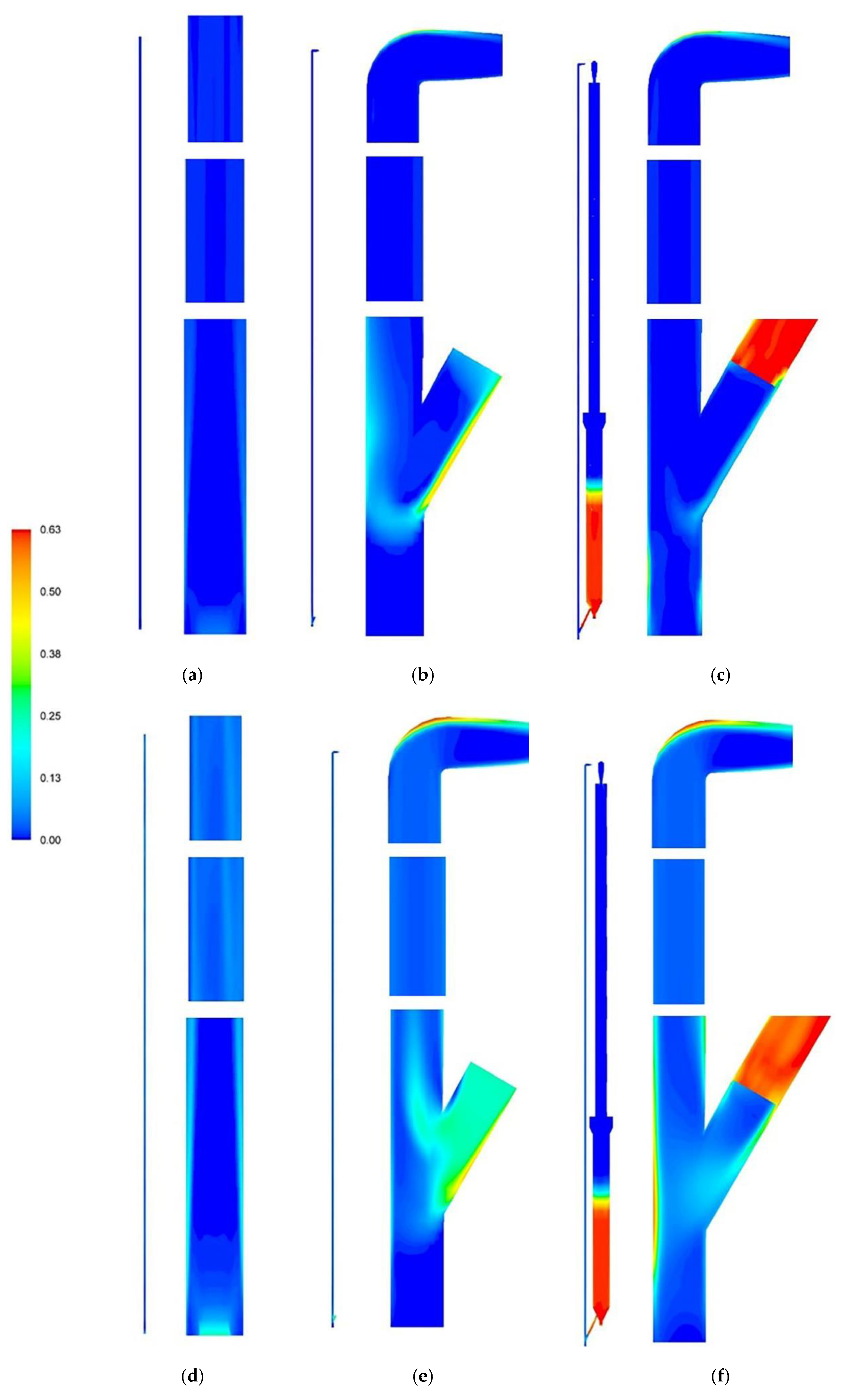
Figure 9 presents the solids holdup contour among different simulations. In the riser-simplified simulation, the effects of both the entrance and exit on hydrodynamics in the riser are neglected. The solids holdup distribution at the bottom and top region of the riser is quite different from the experiment. In the riser-only simulation, particles can flow into the riser in the whole cross section of the feed pipe. A lot of particles flow down along the bottom of the feed pipe into the riser. However, the flow area of the inlet is different in the experiment because of the obstruction of the valve. The particles can only flow through the opening region of the valve, the area of which usually is less than that of the cross section of the pipe, leading to high velocity in the flow region, but low velocity near blocked region. Under different operating conditions, the gas–solids distribution and velocity are different; the riser-only simulation simplifies the inlet boundary condition as a uniform inlet. Hence, the riser-only simulation could not predict the real situation in the inlet of the riser. In the full-loop simulation, the solids holdup distribution in the whole system can be obtained. Lots of particles are packed in the storage tank, which forms a boundary with a relative stable storage height. Particles at bottom of the storage tank that flow into the riser are obstructed by the valve. As a result, solids holdup in the upstream of the valve is much higher than that in the downstream. Through the feed pipe, particles flow into the riser and then upward under the drag force.
Furthermore, through the feed pipe, the particles flow to the opposite wall of the inclined pipe and generate a high solids concentration region. This phenomenon can only be obtained by the full-loop simulation, while in the riser-only simulation, the particle inlet velocity is lower and few particles flow to the opposite wall region. Many particles impact the wall, leading to abrasion and erosion of the wall. Therefore, full-loop simulation is able to analyze the erosion of the wall more accurately.
As for the exit region of the riser, there is little difference between the results of the riser-only and full-loop simulation. When the upward gas–solids flow moves into the elbow at the top of the riser, the particles collide with the outside of the elbow and many particles aggregate near the wall. Both the riser-only and full-loop simulation can catch this phenomenon.
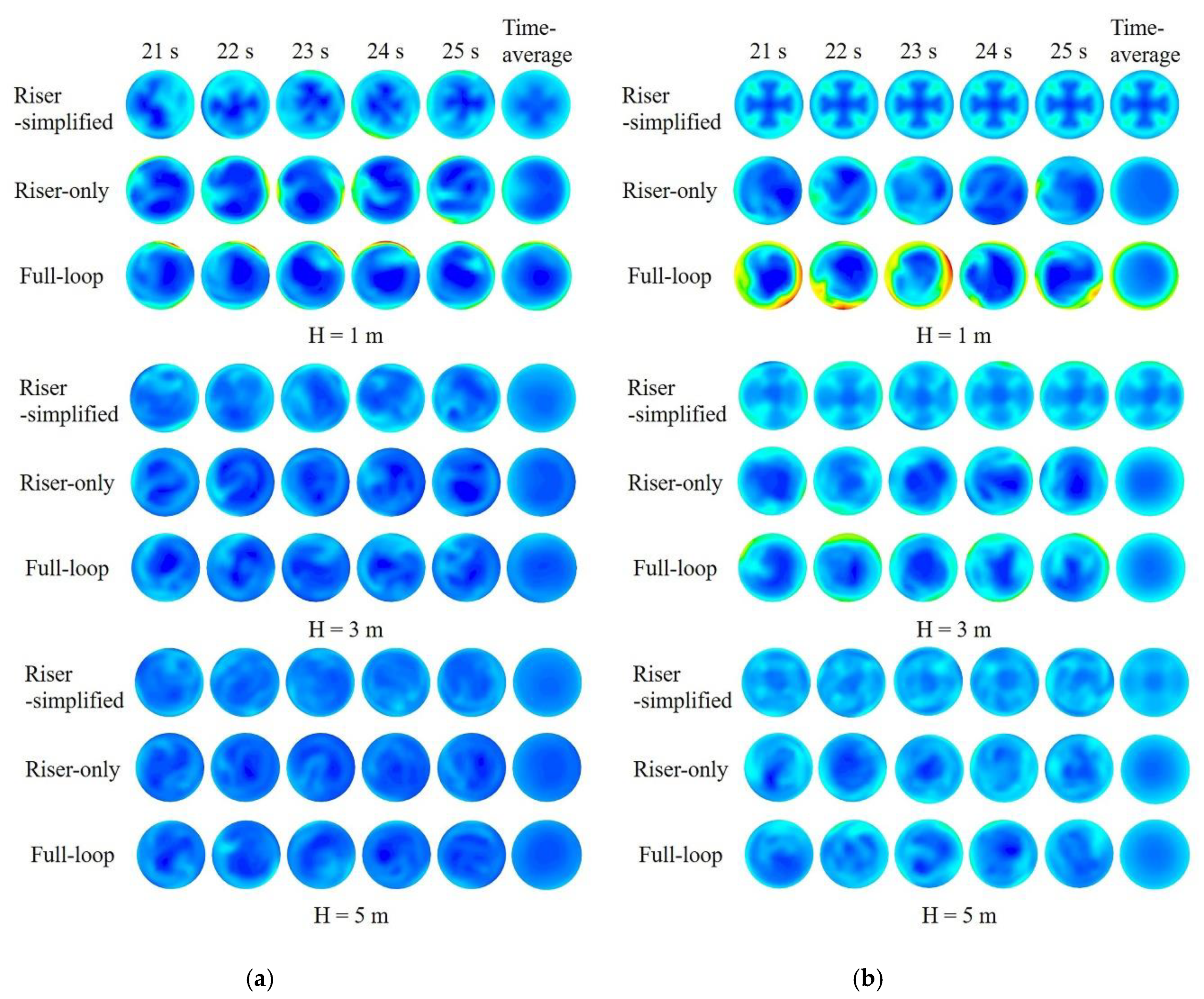
Figure 10 shows a comparison of transient and time-averaged solids holdup in different time in riser between different methods. When Gs = 50 kg m
−2 s
−1, in the cross section of the riser height at 1 m, the solids holdup in the central region in simplified-riser is higher than that in the other two simulations. The solids holdup near the wall region obtained by full-loop simulation is much higher than that in others. When the height is up to 3 m, the difference is limited. When Gs = 300 kg m
−2 s
−1, the difference of transient solids holdup among the different methods becomes neglected until the height of the cross section reaches 5 m. Therefore, the simplification of the riser mainly affects the transient flow characteristics in the lower region of the riser. It can be inferred if the riser is not high enough, the transient solids holdup distribution in the riser-simplified and riser-only simulation may be much different from that in the full-loop simulation. In addition, the effects increase with the increase of solids circulating rates. The differences of the results among the three methods become obvious.
3.4. Effects of Different Methods on Solids Velocity of the Riser
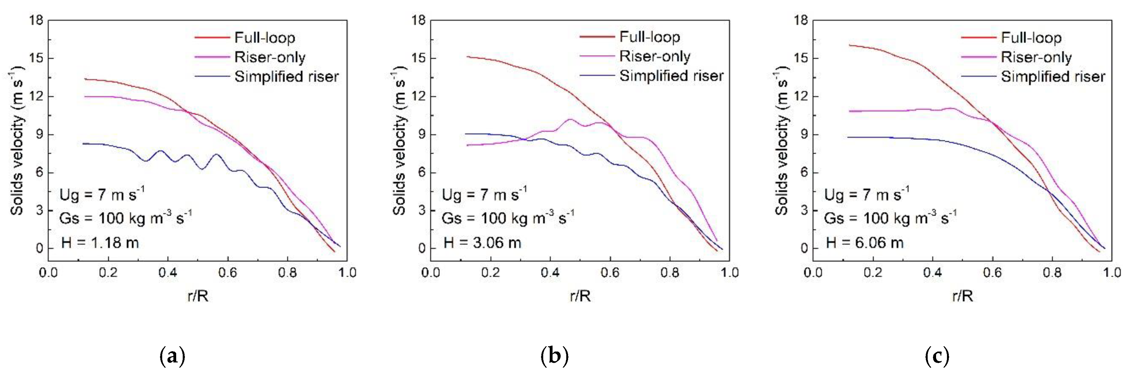
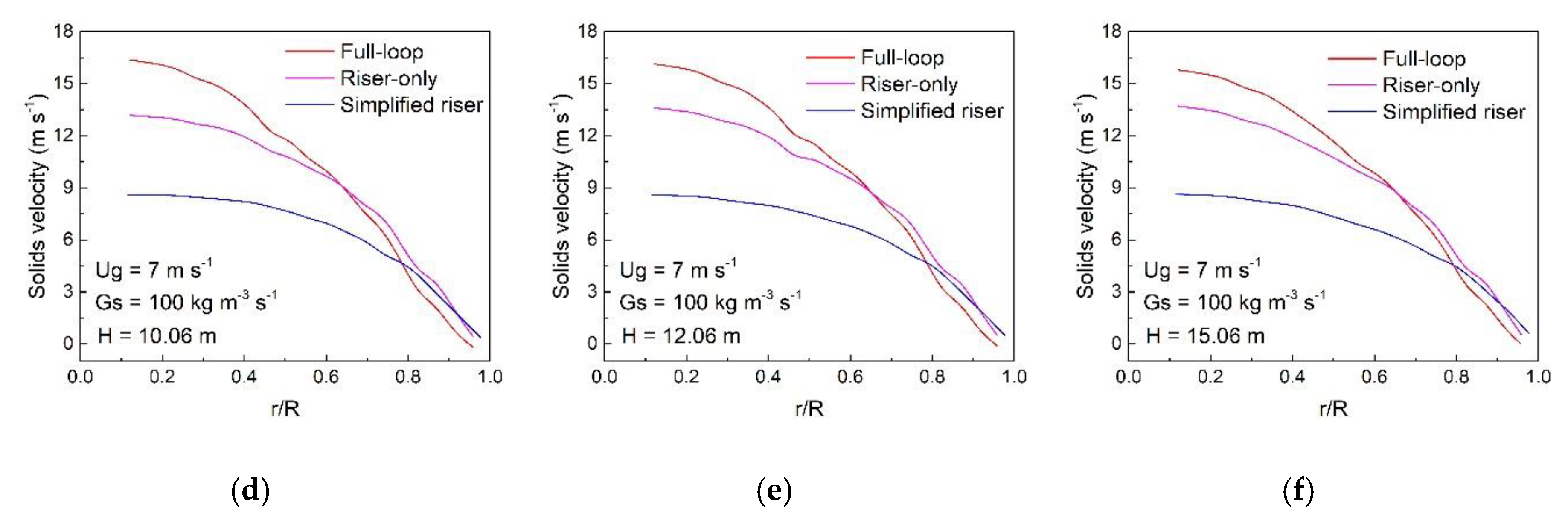
Figure 11 shows the radial distribution solid velocity in the Y direction among different simulations. The solid velocity is highest in the central region of the riser, while it is lowest near the wall because of the intense friction and collision in this region. The solid velocity in the full-loop simulation in the central region is higher than that in the other two simulations, while the solid velocity in the simplified riser is the lowest. Moreover, the difference exits in the whole riser, and the gap does not narrow with the development of the gas–solid flow.
Figure 12 presents the vector of solid velocity in the Y direction among different simulations. In the riser-simplified simulation, though the solid velocity presents parabolic distribution at the bottom of the riser, the solids distribute along the riser, leading to the decrease of the velocity at the center. With the development, the velocity distribution becomes nearly parabolic again. In the riser-only simulation, because of the effects of the inclined feed pipe, particles flow from the inclined pipe to the riser. As a result, many particles collide and reflect with the opposite wall. The velocity at the feed pipe side is larger than at the opposite side. However, in the full-loop simulation, there is a valve in the feed pipe, leading to a non-uniform distribution of the solids. The solids velocity at the opposite side is larger than at the feed pipe side.
In the middle part of the riser, solid velocity in all simulations presents parabolic distribution, but the gap of velocity between the central and near wall region in the full-loop simulation is larger than in the other two.
At the top of the riser, the riser-simplified simulation does not consider the structure of the exit. The velocity distribution near outlet is similar to that in the middle part. The riser-only simulation and full-loop simulation both study the effects of the exit. The solids collide with the wall of the elbow and change the direction. In the full-loop simulation, there are cyclones connected with the outside of the riser, causing a more reliable result. However, the results of the riser-only simulation are also sufficient as the length of the outlet pipe is sufficient.
In higher solids circulating rates, the difference among these simulations is more obvious. Therefore, it is necessary to conduct a full-loop simulation in higher solids circulating rates.
3.5. Comparison of Instantaneous Mass Flow Rates among Different Methods
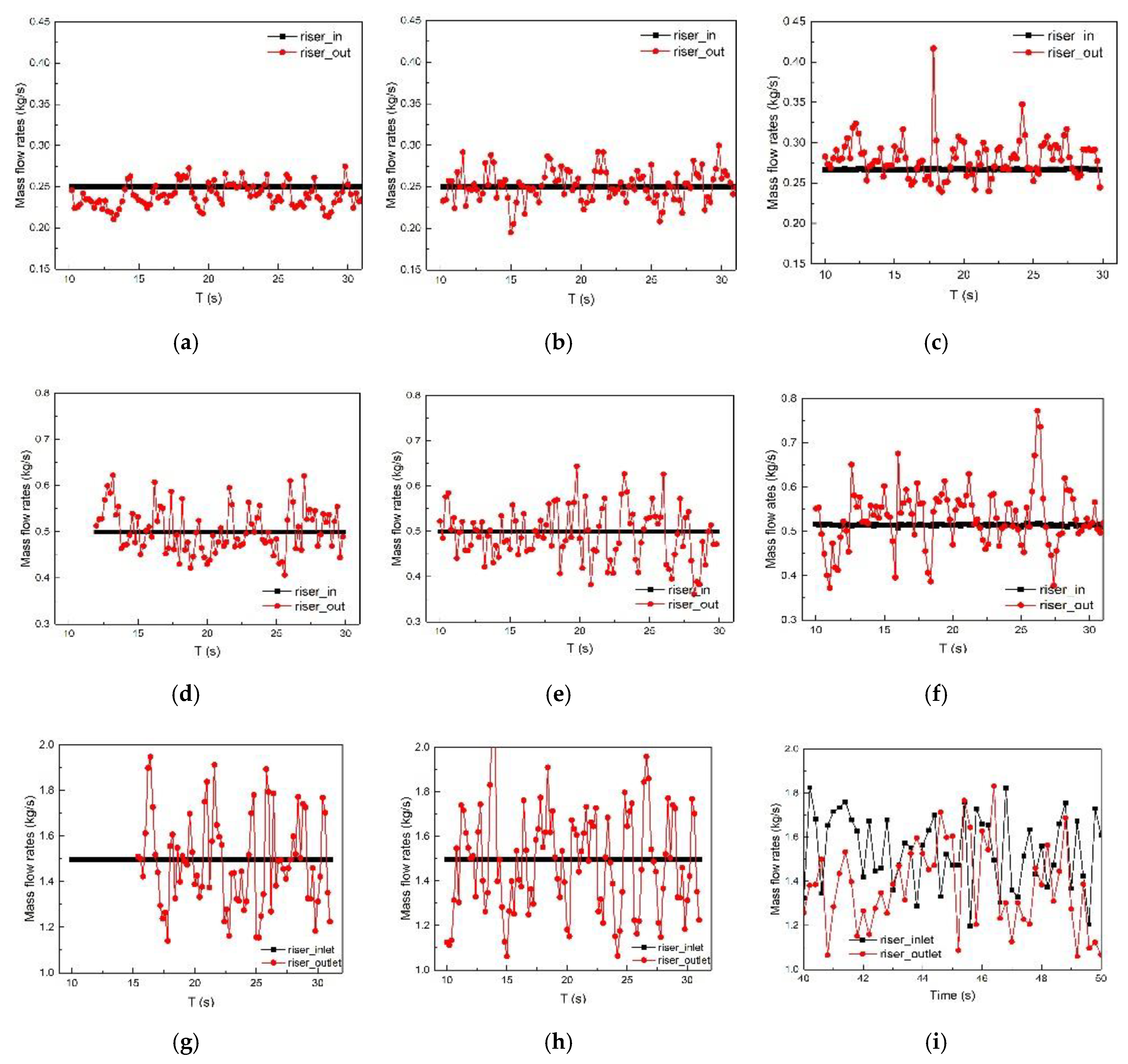
Figure 13 shows the transient mass flow rates in both the inlet and outlet of the riser. In the riser-simplified and riser-only simulation, the Gs in inlet is a constant with no fluctuation, while in the full-loop simulation, the Gs is obtained by calculation. With the increase of Gs, the fluctuation in both the inlet and outlet of the riser increases in full-loop simulation; while only fluctuation in outlet of the riser increases in the riser-only simulation. Higher Gs means more particles move from the storage tank into the riser, leading to more variation of the storage height, which is related to the driving force of the system. Therefore, there is more fluctuation of the solids mass flow rates in higher Gs. However, in the other two simulations, the Gs in the riser inlet is always a constant, which could not reflect the effects of the return system.


