Abstract
It is difficult to manually process and analyze large amounts of data. Therefore, to solve a given problem, it is easier to reach the solution by studying the data obtained from the environment of the problem with computational intelligence methods. In this study, pool boiling heat flux was estimated in the isolated bubble regime using two optimization methods (genetic and artificial bee colony algorithm) and three machine learning algorithms (decision tree, artificial neural network, and support vector machine). Six boiling mechanisms containing eighteen different parameters in the genetic and the artificial bee colony (ABC) algorithms were used to calculate overall heat flux of the isolated bubble regime. Support vector machine regression (SVMReg), alternating model tree (ADTree), and multilayer perceptron (MLP) regression only used the heat transfer equation input parameters without heat transfer equations for prediction of pool boiling heat transfer over a horizontal tube. The performance of computational intelligence methods were determined according to the results of error analysis. Mean absolute error (MAE), root mean square error (RMSE), and mean absolute percentage error (MAPE) error were used to calculate the validity of the predictive model in genetic algorithm, ABC algorithm, SVMReg, MLP regression, and alternating model tree. According to the MAPE error analysis, the accuracy values of MLP regression (0.23) and alternating model tree (0.22) methods were the same. The SVMReg method used for pool boiling heat flux estimation performed better than the other methods, with 0.17 validation error rate of MAPE.
1. Introduction
Pool boiling processes are important heat transfer mechanisms in many engineering applications [1], especially in chemistry, mechanical engineering processes, refrigeration, gas separation, etc. [2]. The formation and removal of vapor bubbles from the solid–liquid interface can be explained by boiling. In the literature, boiling heat transfer studies can be divided into two groups: (1) flow boiling; and (2) pool boiling [3,4]. Boiling allows the transfer of large amounts of heat energy at low-temperature differences. The boiling event has a wide range of applications. The major areas of application include nuclear power plants, rocket motors, refrigeration industry, boilers, steam power units, process industry, and evaporators. Although many investigations are reported on the boiling mechanism, the physical mechanism of boiling has not yet been fully elucidated, even in the case of running water [5]. Many investigators have improved correlation for calculating boiling heat flux [6]. These correlations are calculated for nucleate pool boiling heat flux to nearly 50% error [7,8,9,10]. Nowadays, many investigators study optimization and ANN for heat transfer prediction [11,12,13,14]. Das and Kishor studied the heat transfer coefficient in pool boiling of distilled water. They compared the results of the zero-order adaptive fuzzy model and adaptive neuro-fuzzy inference system (ANFIS function) [15]. Swain and Das used the computational intelligence methods for the flow boiling heat transfer coefficient [16]. Barroso-Maldonado et al. studied cryogenic forced boiling. They compared ANN to three conventional correlations [17].To calculate heat transfer in fluids, some researchers have developed models using computational fluid dynamics [18,19].
In recent years, many researchers have studied the optimization of the heat transfer of the pool boiling [1,20,21]. Many researchers have predicted heat flux with computational intelligence methods. Table 1 depicts the conditions under which the boiling heat transfer is calculated, the algorithms used in heat flux estimation, which error measures are used to determine the accuracy of the predictive models and the error analysis results. There are generally two types of computational intelligence methods: (1) white-box techniques; and (2) black-box techniques. Optimization techniques, such as genetic and ABC, are white-box techniques, while artificial intelligence techniques, such as ANN, DT, and MLP, are black-box techniques.

Table 1.
The predictive models of heat flux in the literature.
In this study, the pool boiling heat flux was calculated by optimizing semi-empirical correlations. Then, heat flux estimation was realized using computational intelligence methods considering the parameters used in the calculation of conventional correlations. These methods were also compared with well-known correlations. To the authors’ best knowledge, this study contributes to the heat flux estimation for pool boiling literature by using black-box techniques for the first time.
2. Pool Boiling Mechanisms in Isolated Bubble Regime Region
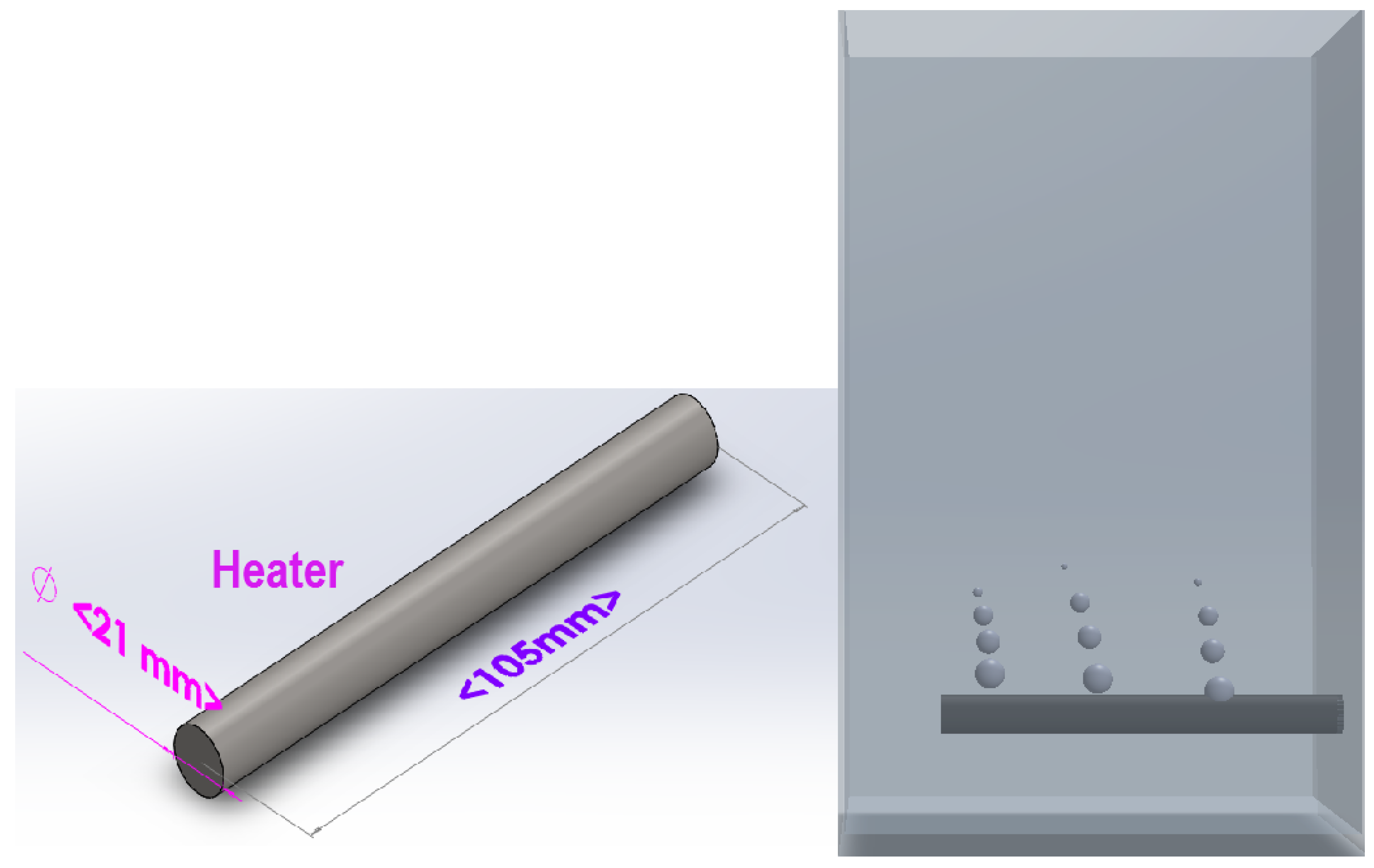
The boiling process occurs when the temperature of the solid surface to which the liquid contacts exceeds the saturation temperature corresponding to the pressure of the liquid. Boiling process is described visually in Figure 1. In Figure 1, the pipe diameter and length are 21 mm and 105 mm, respectively. The experimental heat flow is about 10–80 kW/m. Four different materials, copper, brass, aluminum, and steel, are used as heater surface. The surface roughness is 30–360 mm and the conditions are atmospheric pressure. The vessel of the boiling volume is 0.003 m. Water and ethanol were used for a boiling liquid. As seen in Figure 1, the first bubble was boiled in the boiling core in the isolated bubble regime. However, the bubble did not reach the free surface. In an isolated bubble regime, the boiling core was analyzed for boiling the pool on a horizontal tube heater [20].

Figure 1.
The schematic problem description.
In the region of the isolated vapor bubble, the vapor bubbles do not emerge on the fluid surface and become condensed again by condensation. Although the temperature difference between the fluid and the surface is low in this region, the amount of heat transferred is very high. According to the Fazel study [20], the isolated bubble regime had six mechanisms (microlayer evaporating, transient conduction, bubble super-heating, sliding bubbles for transient conduction, radial forced convection, and natural convection). The model used for optimization in the study is a semi-empirical model that estimates heat flux by a Genetic Algorithm [20]. Fazel’s model, although improved at the isolated bubble regime region, has the following limitations: (1) the heat transfer is one dimensional; (2) bubbles are adopted in a spherical shape; (3) tThe heater temperature is constant; (4) bubbles are isolated, i.e., there are no bubble interactions; and (5) the physical properties do not change [20]. The boiling heat transfer model as the sum of the six mechanisms is written below.
Microlayer evaporating equation [22]:
Transient conduction equation [22]:
Bubble super-heating equation [20]:
Sliding bubbles for transient conduction equation [20]:
Radial rorced convection equation [20]:
Natural convection equation [23,24]:
The above equations and experimental data were taken from Fazel’s work (see the article for more details) [20]. The pool boiling heat transfer is affected by many parameters that are easily obtained from correlations given in the literature: the wall temperature (), evaporation temperature (), bubble departure diameter (d), bubble frequency (f), nucleation site density (NA), latent heat vaporization (), liquid density (), vapor density (), liquid heat capacity (), vapor heat capacity (), dynamic viscosity , Prandtl number (Pr), liquid thermal conductivity (), Grashoff number (Gr), and vapor thermal conductivity (). These parameters are used to calculate the pool boiling heat flux (q/A). q/A is the total of the six mechanisms of heat flux equations. These parameters are available for computational intelligence technique as well.
3. Computational Intelligence Methodology
In a mathematical approach, most optimization methods investigate the places where the function is zero and the places where the derivative is zero. The derivative calculation is not always an easy task. Many of the technical problems can be formulated to find their roots. However, some optimization methods fail to find these roots. Another challenge in optimization is determining whether a result is a global or local solution. Such problems are solved either by a linear approach or by limiting the bounds of the optimization domain. In this study, five different computational intelligence methodologies were selected to estimate pool boiling heat transfer in isolated bubble regime.
3.1. Genetic Algorithm
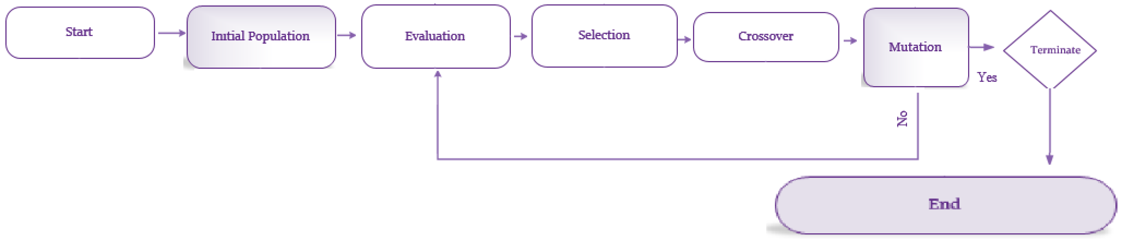
Genetic Algorithm is the first and most known of the evolutionary calculation algorithms. To understand the terminology of the genetic algorithm (GA), it is necessary to understand natural selection. When observing the world, natural selection comes to the fore in events. The enormous organisms and complexity of these organisms are the subject of investigation and research. It can be questioned why organisms are like this and how they come to this stage. The level of adaptation and suitability has become a sign of long-term survival in the world. The process of evolution is a great algorithm that allows the most appropriate life conditions. If an organism has the intelligence and ability to change the environment, the global maximum can be achieved in life [34]. This algorithm externalizes the process of natural selection in which pertinent individuals are selected for reproduction to produce progeny of the next generation. General flow chart of the genetic algorithm is given in Figure 2.
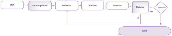
Figure 2.
Genetic algorithm steps.
3.2. ABC Algorithm
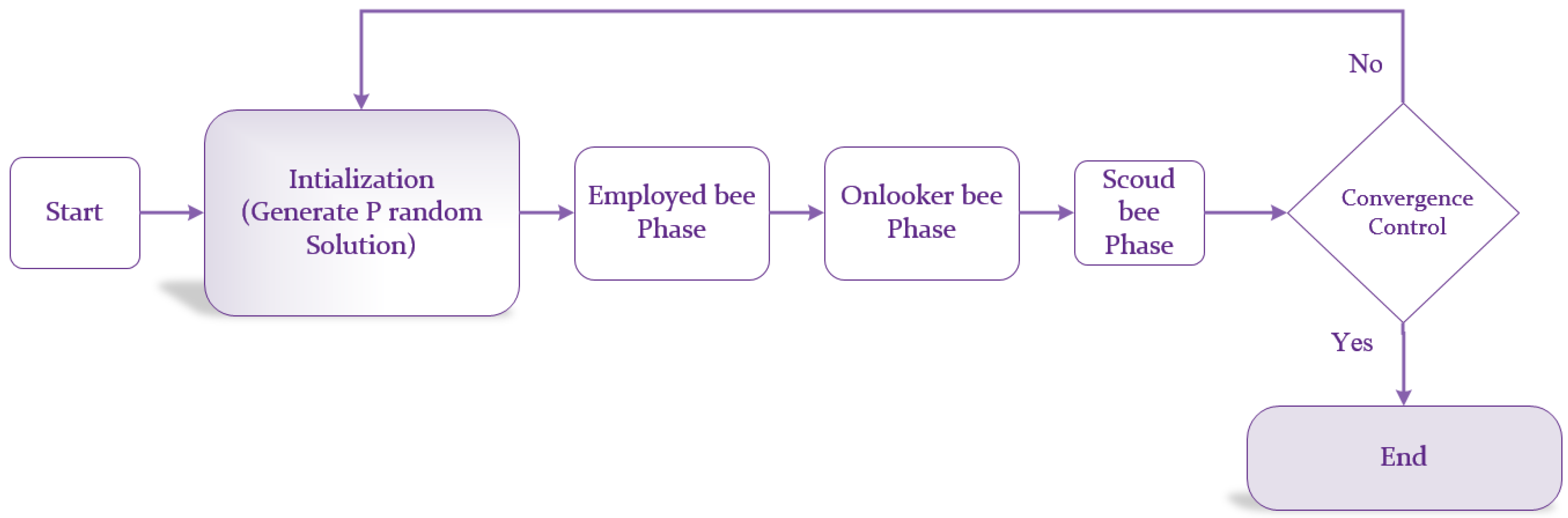
ABC algorithm is the modeling of bees food search mechanisms. The bees live in colonies. The bees colony includes three groups of bees: onlookers, scouts, and employed bees. Some of the colony consists of employed artificial bees and the others contain onlookers. For each food source, there is solely an employed bee [35,36]. Figure 3 shows the main steps for the ABC algorithm. In this study, the ABC algorithm and the GA algorithm were used with the same mathematical model and bounds; however, their configurations were different. Both algorithm configurations are shown in Table 2.
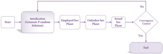
Figure 3.
ABC algorithm steps.
Table 2.
Configuration of both algorithms.
The optimization model was based on 18 parameters: (1) q/A; (2) ; (3) ; (4) d; (5) NA; (6) f; (7) ; (8) ; (9) ; (10) ; (11) ; (12) ; (13) ; (14) ; (15) ; (16) Gr; (17) Prandtl; and (18) Ra roughness. Some of these parameters were obtained from experiments: (1) ; (2) ; (3) d; (4) NA; (5) Ra; and (6) f. The rest of the datasets were obtained from an EES package program: (1) ; (2) ; (3) ; (4) ; (5) ; (6) ; (7) ; (8) ; (9) ; and (10) Prandtl. If these datasets were used as the input parameter, for the computational intelligence algorithms, boiling heat flux (q/A) could be estimated. The boiling fluid thermophysical properties were evaluated at the arithmetic mean of the saturated fluid and heater surface temperature, defined by Equation (20).
3.3. Support Vector Machine Regression
Support vector networks, which are a variety of universal feeder networks, were developed by Vapnik and Cortes [37] to classify data and are generally referred to as support vector machines (SVM) in the literature. The SVM-based model for regression is called the support vector regression (SVMReg) [38]. SVR uses not only empirical risk minimization but also the principle of structural risk minimization, which is intended to reduce the upper limit of the generalization error, compared to traditionally controlled learning methods of neural networks. Thanks to this principle, the SVR has good generalization performance for previously untested test data using the learned input–output relationship during the training phase. Consider the expression vector for the problem of approach to a continuous-valued function. The expression , which is a set of N numbers, indicating the output (target) value. The aim of the regression analysis is to determine a mathematical function to accurately predict the desired (target) outputs (). The regression problem can be classified as linear and nonlinear regression problems. Since the problem of nonlinear regression is more difficult to solve, SVMReg is mainly developed for the solution of nonlinear regression problem [39]. To solve the nonlinear regression problem, the SVM carries the training data in the “i” input space to the higher-dimensional space with the help of a nonlinear function and applies linear regression in this space. In this case, the mathematical representation of the linear function obtained to find the best regression is as follows [39]:
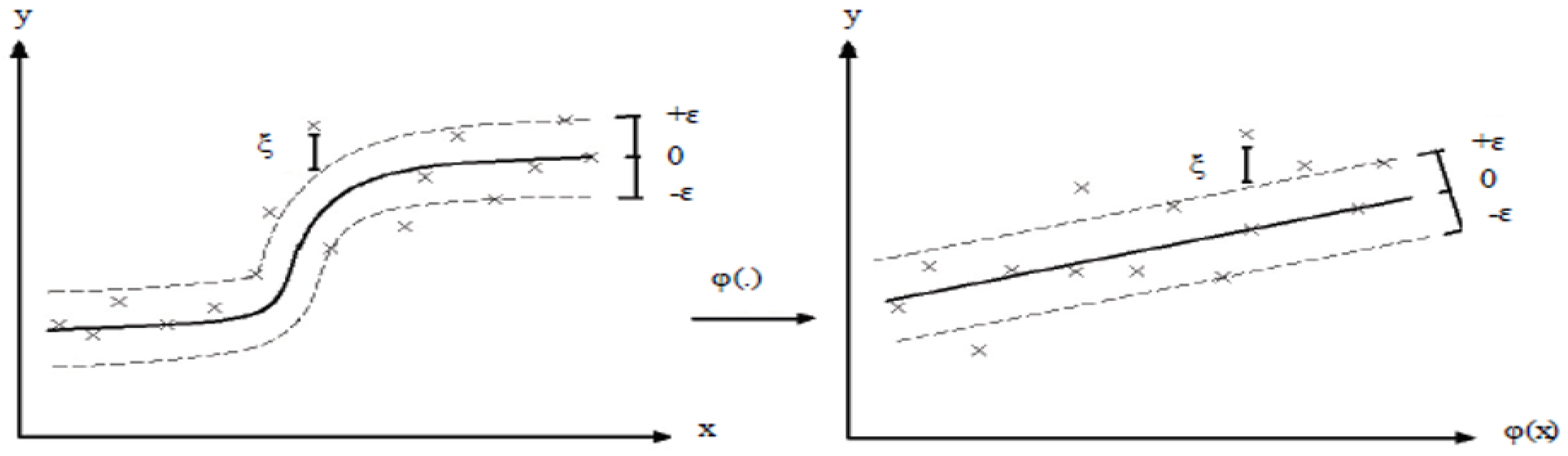
where represents the model parameter vector and represents the deviation term in the vertical axis. Thus, the linear regression obtained by the inner product between and (x) in the higher-dimensional space corresponds to the nonlinear regression in the input space (Figure 4). The objective function of the SVR, which performs linear regression in high-dimensional space, is usually composed of a -insensitive loss function and minimization of the parameters representing the model in Equation (22).
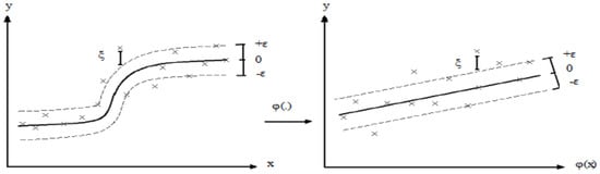
Figure 4.
Using the nonlinear function (.) mapping training examples in the input space to a high dimension where they are linear.
Here, the first term represents the square of the Euclidean norm of the model parameters, the second term is the experimental error (loss) function, and the is a positive constant number. The task of C is to maintain a balance between the experimental error and the extreme compatibility of the model with the training data. Small C values give more importance to the optimization problem in contrast to the experimental error, while the higher C values give more importance to the reduction of experimental education error than the norm of [39]. SVM regression computational intelligence method was used to create a predictive model of q/A values calculated by experimental data. This method was done with the SMOreg toolbox in WEKA 3.8.3. WEKA is open source software. There are many algorithms in this software, which include classification, estimation and clustering rules. It is necessary to define the kernel function to be used for a classification to be performed by SVM and optimum parameters of this function [40]. The most widespread used radial basis function (RBF) kernels in the literature are presented together with formulas and parameters in Equation (23). Batch size is 1000. “C” is 200.0. Filter type is standardized.
3.4. Multilayer Perceptron
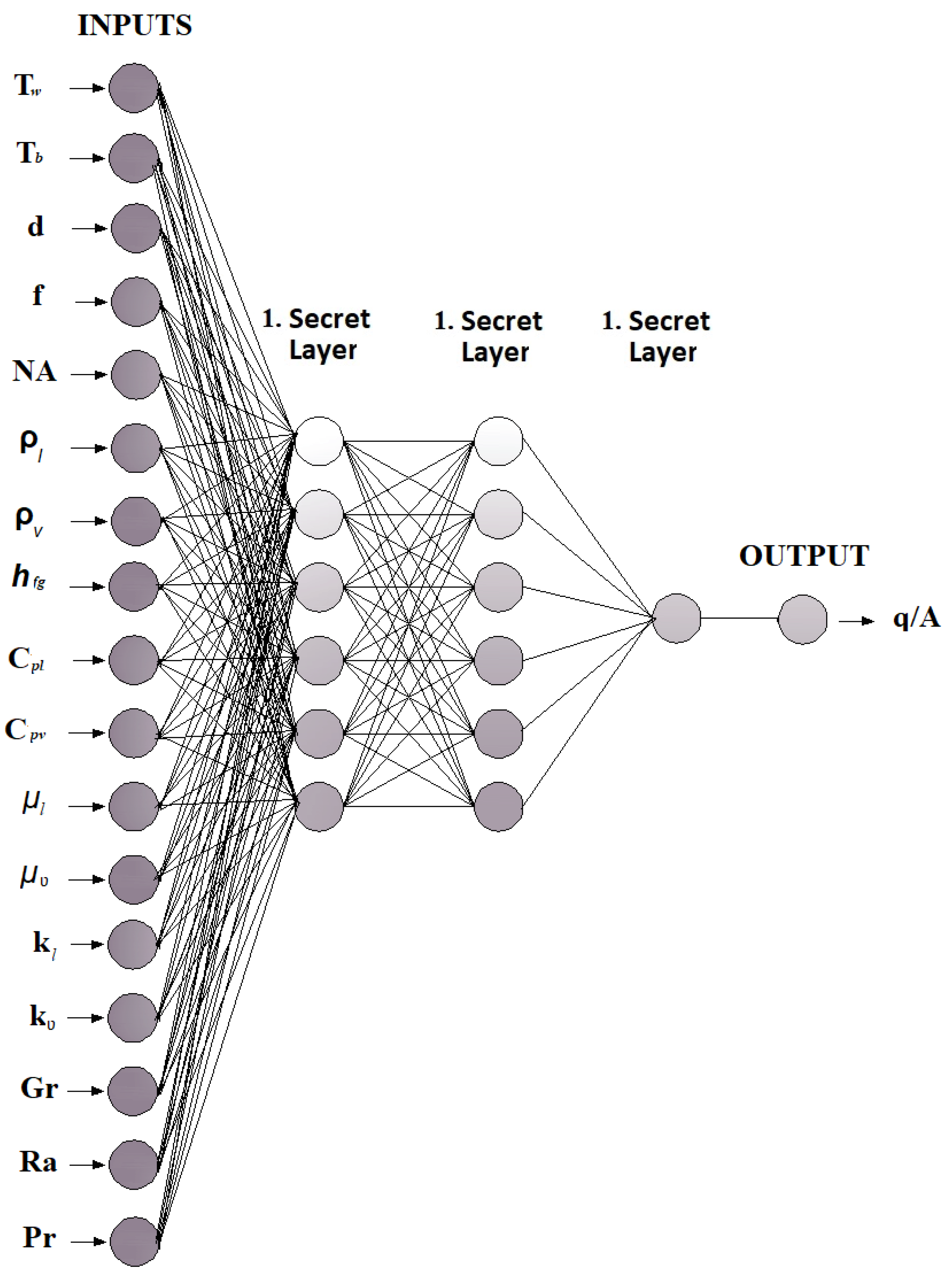
Artificial intelligence has been brought to science through long-term studies to model the human brain. Then, the artificial neural networks (ANN) method was developed by means of these studies. The ANN technique achieved reliable results in nonlinear equation solutions and its use has become increasingly widespread over time. In the ANN method, models with a multi-layer perceptron (MLP) are generally used for classification and regression approaches. The software application of the MLP neural networks is used in the algorithm development phase and in cases where parallel-low delay approaches are not required. In many applications in the literature, rapid data processing, and low delays are required by the ANN method. To supply this need, MLP is used as an ANN method consisting of multiple neural layers in a feed-through network. The MLP consists of three or more layers consisting of one inlet, one outlet, and one or more hidden layers. Because the MLP is a fully connected network, each neuron contained in each layer is associated with the next layer with a certain weight value. The MLP method uses a controlled learning method called backpropagation. In MLP, the weight function is defined in the training phase of the neural network [41]. As a middle layer, six hidden layers were created and the best solutions were tried by changing the number of intermediate layers. The structure of the generated MLP model is given in Figure 5.
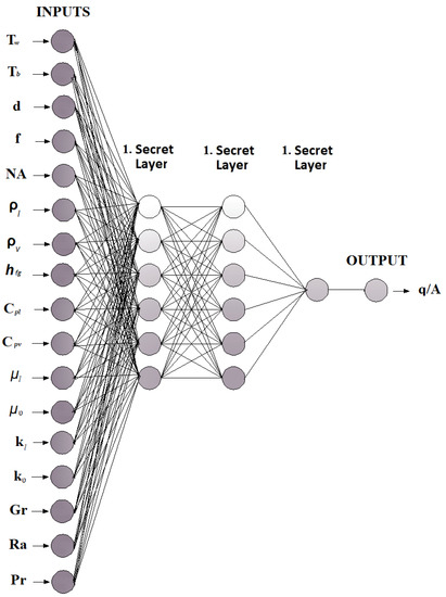
Figure 5.
MLP structure.
Prediction of q/A values with MLP was done using WEKA 3.8.3 software. The MLP network structure used for estimation of q/A is shown in Table 3.
Table 3.
The Network structure of MLP.
3.5. Alternating Decision Tree
Decision trees, which are a strong regression method, have a clear concept description for a dataset. The decision tree learning method is a popular method because of its fast data processing capability and because it produces successful performance predictive models [42,43]. The alternative decision tree (ADTree) method consists of decision nodes and prediction nodes. Each action in the decision nodes indicates the result. The prediction nodes contain a single number value. The ADTree method always contains prediction nodes, which consist of both root and leaves. When regression or classification is done by the ADTree method, the paths of all decision nodes and prediction nodes are monitored [44]. In the ADTree method, the learning algorithm must be 1 <= i <= n. In this expression, n is provided via a sample . In this sample, xi indicates an attribute value indicating the vector and yi indicates the target value. For this dataset, when a different vector x is entered, this model is used to estimate the value corresponding to the y value. The purpose of the ADTree model is to minimize the error between the actual value and the estimated value. The ADTree method uses the basic algorithm of incremental regression by using the advanced stepwise additive model at the stage of learning additive model trees [45]. If a model consisting of k base model is created,
the error squared on a progressive state,
is minimized through n training samples.
As input data for the all regression analysis model, the following were used: (1) ; (2) ; (3) d; (4) NA; (5) f; (6) ; (7) ; (8) ; (9) ; (10) ; (11) ; (12) ; (13) ; (14) ; (15) Gr; (16) Prandtl; and (17) Ra roughness values. Boiling heat flux (q/A) was used as output data.
All numerical method errors were calculated for MAE, MAPE, and RMSE. All error calculation methods are shown in Table 4.
Table 4.
Some error equations.
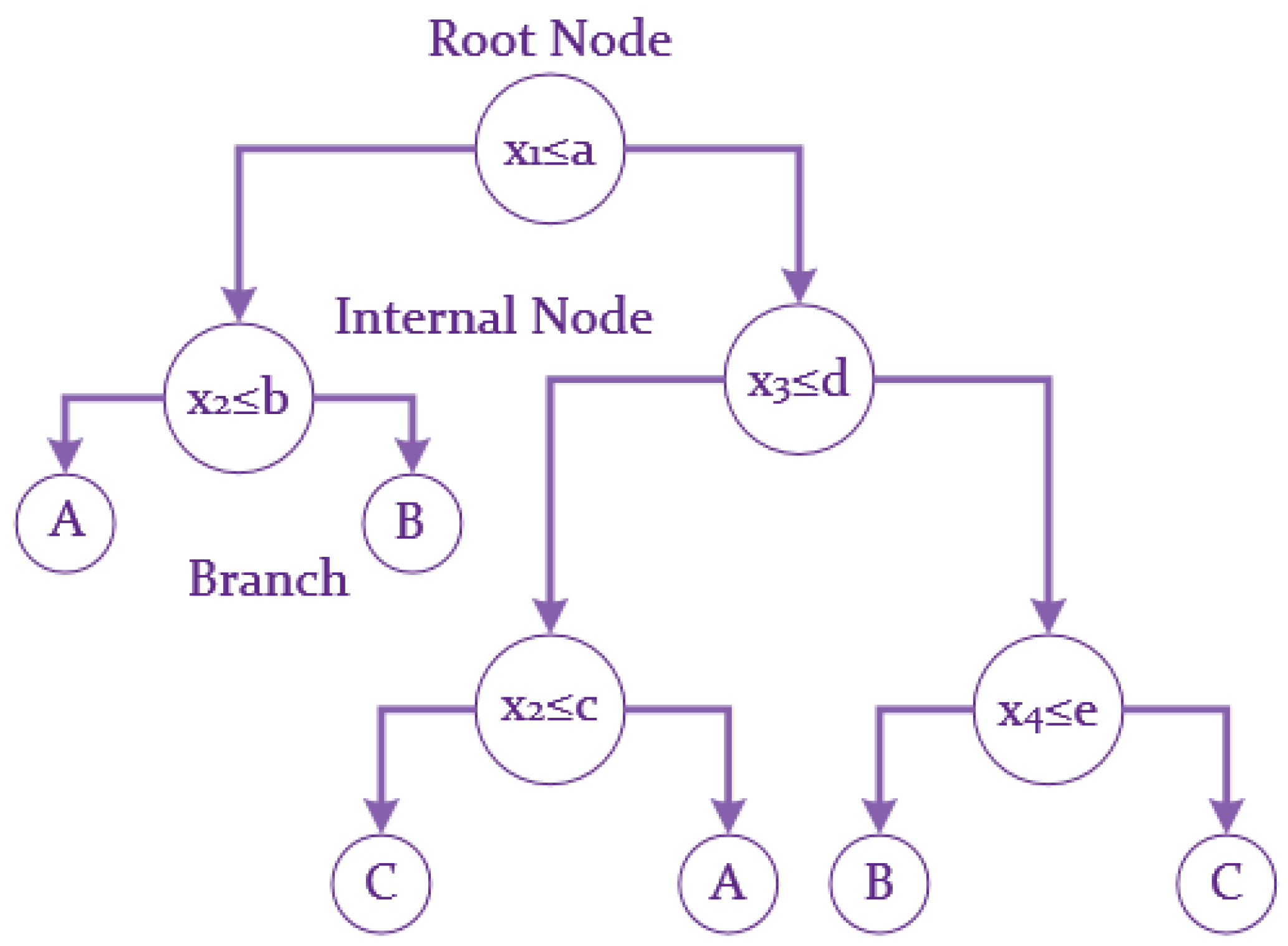
The test dataset is used to determine the generalization capability of the generated tree for a new dataset. A test data coming from the root of the tree enters the tree structure created with the training dataset. This new data tested in the root is sent to a lower node according to the test result. This process is continued until it reaches a specific leaf of the tree. There is only one way or a single decision rule from root to every leaf [46]. The working principle of the decision tree method, which is a computational intelligence method, is simply shown in Figure 6. Figure 6 shows a simple tree structure consisting of four-dimensional attribute values of three classes. In the Figure 6, the xi parameter shows the values of the attribute. The parameters a, b, c, and d show the threshold values in tree branches. Parameters A, B, and C show the class label values [47].
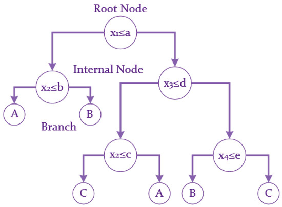
Figure 6.
A decision tree structure consisting of three classes with four-dimensional property space.
4. Results
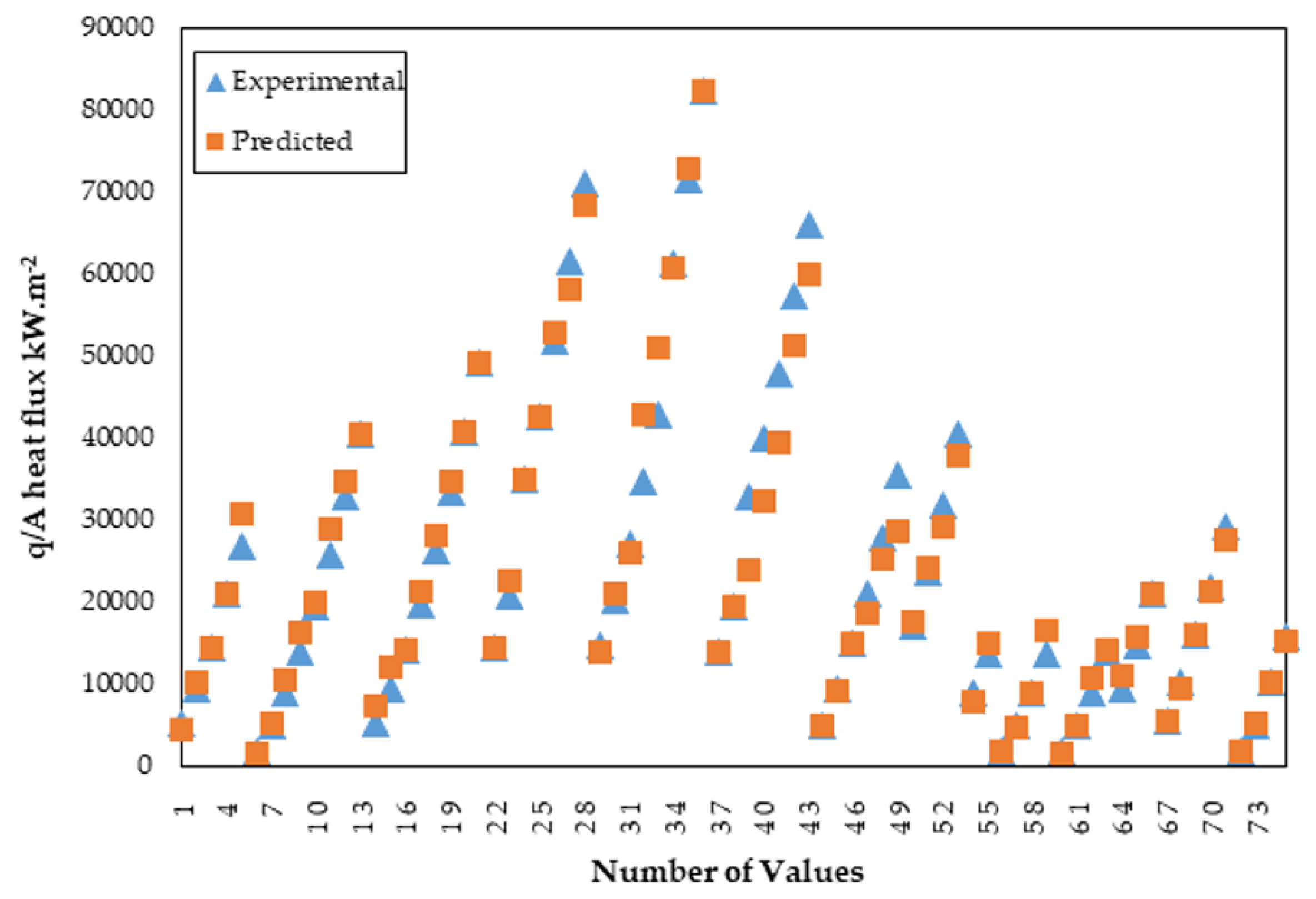
Five different computational intelligence methods were applied to predict pool boiling heat transfer phenomena. Genetic and ABC algorithms are both white-box algorithms, in which the internal structure, design, and implementation of the item being tested are known to the tester. All parameters required for algorithms were obtained from Fazel [20]. The black-box technique is the opposite of the white-box technique and its algorithms cannot be changed. They can only be partially modified for the prediction, for example the learning rate, momentum, batch size, and Figure 7 shows the predicted output of the SVMReg. In the figure, it can be seen that the predicted output of the SVMReg and experimental data are mostly in agreement.

Figure 7.
The SVMReg forecast.
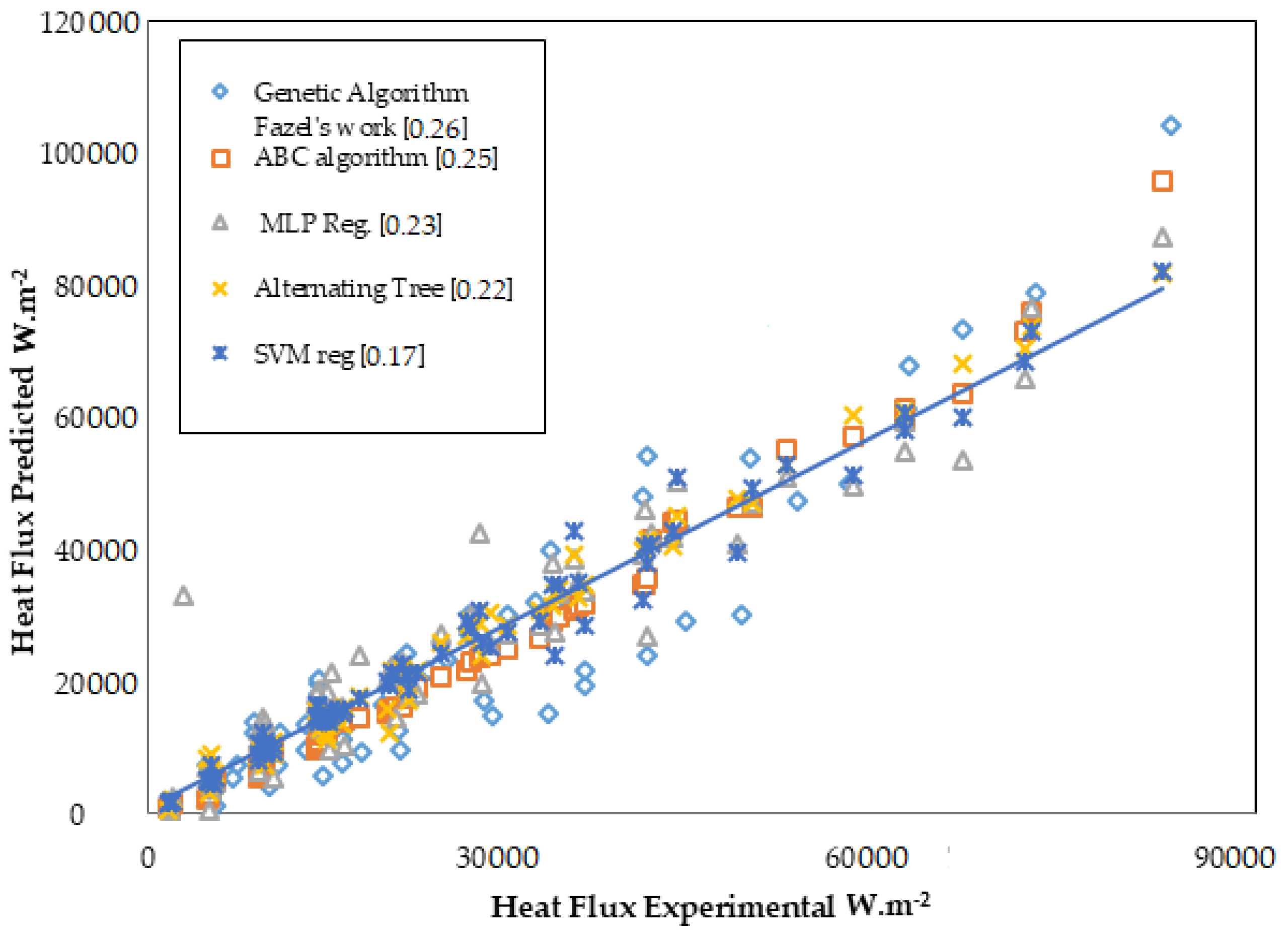
Figure 8 shows a comparison of the black-box techniques to white-box techniques. The apsis is the experimental results, and the ordinates are the predicted models. The figure shows that both algorithms predictions were nearby the 0.25 mean absolute percentage error of the actual result. MLP and Alternating tree had unequal distributions, whereas SVMReg prediction was slightly more stable than the others. Therefore, its mean absolute percentage error was less than all other methods. SVMReg model performed better than the other methods.
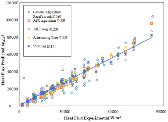
Figure 8.
The comparison of black-box techniques to white-box techniques.
Seventeen attributes (1275) were used for analysis. An attribute q/A (75) was selected to be used as the solution class. In this study, the ten-fold cross-validation technique was applied to process the data with less error rate in machine learning algorithms. Cross-validation is a technique used in model selection to better estimate the error of a test in a machine learning model. In cross-validation, the training data are divided into subsets. A subset is used for training, and the remaining sets are used for validation. This process is repeated for all subsets in a crossway. This is done for k presets. In the literature, ten-cross validation can be seen in many articles [33,48]. Data are divided into k pieces of equal length and evaluated k times. The mean absolute error (MAE), root mean squared error (RMSE) and mean percentage error (MAPE) are shown in Table 5.
Table 5.
Error rates for all methods.
Instant heat flux has to be estimated in pool boiling. This requirement is mainly for determining the boiling heat transfer coefficient. Figure 9 depicts the results of the well-known correlations and computational intelligence techniques used in the study. It is clearly seen that the computational intelligence techniques performed better than the correlations developed. Especially, SVMReg predicted q/A error rate with a MAPE nearby 0.17. This error rate was the minimum value presented in this study. In this analysis, some parameters were obtained as a result of experiments. The other parameters were obtained from EES. However, they could make better predictions than the many correlations used today for the development of data. In the near future, computational intelligence techniques can be used more in predicting the heat transfer of boiling phenomena. Some researchers supported this view in their works [49,50,51].
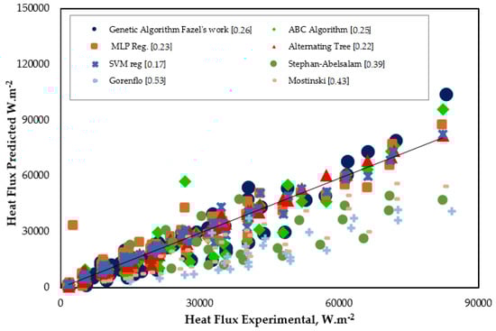
Figure 9.
Comparison of some well-known correlation and computational intelligence techniques.
In this study, heat flux estimation was performed using computational intelligence methods during boiling in the isolated bubble regime region. After this study, these methods of computational intelligence can be tried in the boiling zone, where the steam bubble flows to the surface of the fluid, for the transition to boiling, and in the film boiling. In addition, these methods can be tried to estimate the heat transfer coefficient in boiling heat transfer. It is thought that these methods will be successful in estimating the heat transfer coefficient. Thus companies that produce heat exchangers for the industry could benefit from these algorithms in their heat exchanger capacity estimation. The prediction results obtained by these algorithms were found to be better than those obtained with the known correlations.
5. Conclusions
The novelty of this study was to predict the boiling heat flux of a pool by using black-box techniques. Pool boiling heat transfer was predicted with computational intelligence techniques. These computational intelligence methods were Genetic algorithms, ABC algorithms, SVM, DT, and MLP. The predicted heat flux was compared to some well-known correlations. The white-box techniques performance (Genetic and ABC) was limited to the used empirical model, whereas predictions made by black-box techniques (SVM, DT, and MLP) were more successful. Validation error (MAPE) rate of the models were: GA, 0.26; ABC, 0.25; MLP, 0.23; DT, 0.22; and SVM, 0.17. SVMReg was proposed as the best of the models used in the study to predict the heat transfer phenomenon in pool boiling. This study also showed the basics of how to use computational intelligence techniques in engineering calculation programs. By making an addendum to engineering equation solvers such as EES, the ability to use computational intelligence techniques can be improved, more data can be obtained with different boiling techniques, and less erroneous predictive models can be obtained using different computational intelligence methods.
Author Contributions
O.K. supervised all aspects of the research. E.A. and M.D. developed computational intelligence methods and wrote the paper.
Funding
There was no funding for this study.
Acknowledgments
There are no acknowledgments for this study.
Conflicts of Interest
The authors declare no conflict of interest.
Abbreviations
The following abbreviations are used in this manuscript:
| A | Area (m) |
| Average Absolute Relative Error | |
| Alternative Decision Tree | |
| Artificial neural network | |
| C | Batch size |
| The particular area engaged by the bubbles over heater surface area | |
| The particular area engaged by the sliding bubbles over heater surface area | |
| The particular area over the area at which transient heat conduction takes | |
| Various of and | |
| Heat capacity | |
| Decision tree | |
| E | The relative error (%) |
| f | The frequency of bubble separation (Hz) |
| Dimensionless Grashoff number | |
| h | Heat flux watt per square metre (W m) |
| Specific heat of vaporization (J kg) | |
| k | Thermal conductivity (W m K) |
| Mean absolute error | |
| Mean absolute percentage error | |
| Mean squared error | |
| Multilayer perceptatron | |
| Nucleation site density | |
| Natural convection | |
| The Nusselt number | |
| P | Optimization parameter |
| Sum of heat flux (W m) | |
| Radial basis function | |
| Reynolds number | |
| Root mean square error | |
| Support vector machine | |
| Support vector regression | |
| T | Temperature (K) |
| Greek symbols | |
| Density (kg m) | |
| Viscosity (kg m) | |
| Pearson width parameters | |
| Kernel dimension | |
| Subscripts or superscripts | |
| Sliding length (m) | |
| b | Bulk |
| Bubble super-heating | |
| d | The diameter of bubble separation (m) |
| v | Vapor |
| l | Liquid |
| Micro-layer evaporation | |
| Heater outside diameter (m) | |
| Radial forced convection | |
| s | Saturation temperature |
| Thermocouple location | |
| Transient conduction | |
| w | Wall |
References
- Ahn, H.S.; Sathyamurthi, V.; Banerjee, D. Pool Boiling Experiments ona Nano-structured surface. IEEE Trans. Compon. Packag. Technol. 2009, 32, 156–165. [Google Scholar]
- Kandlikar, S.G. Handbook of Phase Change: Boiling and Condensation; CRC Press: Boca Raton, FL, USA; Routledge: Abingdon, UK, 1999. [Google Scholar]
- Yan, B.H.; Wang, C.; Li, R. Corresponding principle of critical heat flux in flow boiling. Int. J. Heat Mass Transf. 2019, 136, 591–596. [Google Scholar] [CrossRef]
- Colgan, N.; Bottini, J.L.; Martínez-Cuenca, R.; Brooks, C.S. Experimental study of critical heat flux in flow boiling under subatmospheric pressure in a vertical square channel. Int. J. Heat Mass Transf. 2019, 130, 514–522. [Google Scholar] [CrossRef]
- Chai, L.H.; Peng, X.F.; Wang, B.X. Nonlinear aspects of boiling systems and a new method for predicting the pool nucleate boiling heat transfer. Int. J. Heat Mass Transf. 2000, 43, 75–84. [Google Scholar] [CrossRef]
- Zahedipoor, A.; Faramarzi, M.; Eslami, S.; Malekzadeh, A. Pool boiling heat transfer coefficient of pure liquids using dimensional analysis. J. Part. Sci. Technol. 2017, 3, 63–69. [Google Scholar]
- Gorenflo, D. Pool Boiling, VDI-Heat Atlas; VDI-Verlag: Dusseldorf, Germany, 1993. [Google Scholar]
- Stephan, K.; Abdelsalam, M. Heat-transfer correlations for natural convection boiling. Int. J. Heat Mass Transf. 1980, 23, 73–87. [Google Scholar] [CrossRef]
- McNelly, M.J. A correlation of rates of heat transfer to nucleate boiling of liquids. J. Imp. Coll. Chem. Eng. Soc. 1953, 7, 18–34. [Google Scholar]
- Mostinski, I.L. Application of the rule of corresponding states for calculation of heat transfer and critical heat flux. Teploenergetika 1963, 4, 66–71. [Google Scholar]
- Chang, W.; Chu, X.; Fareed, A.F.B.S.; Pandey, S.; Luo, J.; Weigand, B.; Laurien, E. Heat transfer prediction of supercritical water with artificial neural networks. Appl. Therm. Eng. 2018, 131, 815–824. [Google Scholar] [CrossRef]
- Esfe, M.H.; Arani, A.A.A.; Badi, R.S.; Rejvani, M. ANN modeling, cost performance and sensitivity analyzing of thermal conductivity of DWCNT-SiO2/EG hybrid nanofluid for higher heat transfer: An experimental study. J. Therm. Anal. Calorim. 2018, 131, 2381–2393. [Google Scholar] [CrossRef]
- Hojjat, M. Modeling heat transfer of non-Newtonian nanofluids using hybrid ANN-Metaheuristic optimization algorithm. J. Part. Sci. Technol. 2018, 3, 233–241. [Google Scholar]
- Harsha Kumar, M.K.; Vishweshwara, P.S.; Gnanasekaran, N.; Balaji, C. A combined ANN-GA and experimental based technique for the estimation of the unknown heat flux for a conjugate heat transfer problem. Heat Mass Transf. 2018, 54, 3185–3197. [Google Scholar]
- Das, M.K.; Kishor, N. Adaptive fuzzy model identification to predict the heat transfer coefficient in pool boiling of distilled water. Expert Syst. Appl. 2009, 36, 1142–1154. [Google Scholar] [CrossRef]
- Swain, A.; Das, M.K. Artificial intelligence approach for the prediction of heat transfer coefficient in boiling over tube bundles. Proc. Inst. Mech. Eng. Part C 2014, 228, 1680–1688. [Google Scholar] [CrossRef]
- Barroso-Maldonado, J.M.; Montañez-Barrera, J.A.; Belman-Flores, J.M.; Aceves, S.M. ANN-based correlation for frictional pressure drop of non-azeotropic mixtures during cryogenic forced boiling. Appl. Therm. Eng. 2019, 149, 492–501. [Google Scholar] [CrossRef]
- Moradikazerouni, A.; Afrand, M.; Alsarraf, J.; Wongwises, S.; Asadi, A.; Nguyen, T.K. Investigation of a computer CPU heat sink under laminar forced convection using a structural stability method. Int. J. Heat Mass Transf. 2019, 134, 1218–1226. [Google Scholar] [CrossRef]
- Moradikazerouni, A.; Afrand, M.; Alsarraf, J.; Mahian, O.; Wongwises, S.; Tran, M.-D. Comparison of the effect of five different entrance channel shapes of a micro-channel heat sink in forced convection with application to cooling a supercomputer circuit board. Appl. Therm. Eng. 2019, 150, 1078–1089. [Google Scholar] [CrossRef]
- Alavi Fazel, S.A. A genetic algorithm-based optimization model for pool boiling heat transfer on horizontal rod heaters at isolated bubble regime. Heat Mass Transf./Waerme- und Stoffuebertragung 2017, 53, 2731–2744. [Google Scholar] [CrossRef]
- Alic, E.; Cermik, O.; Tokgoz, N.; Kaska, O. Optimization of the Pool Boiling Heat Transfer in the Region of the Isolated Bubbles using the ABC Algorithm. J. Appl. Fluid Mech. 2019, 12, 1241–1248. [Google Scholar]
- Benjamin, R.J.; Balakrishnan, A.R. Nucleate pool boiling heat transfer of pure liquids at low to moderate heat fluxes. Int. J. Heat Mass Transf. 1975, 39, 2495–2504. [Google Scholar] [CrossRef]
- Sateesh, G.; Das, S.K.; Balakrishnan, A.R. Analysis of pool boiling heat transfer: Effect of bubbles sliding on the heating surface. Int. J. Heat Mass Transf. 2005, 48, 1543–1553. [Google Scholar] [CrossRef]
- Churchill, S.W.; Chu, H.H.S. Correlating equations for laminar and turbulent free convection from a vertical plate. Int. J. Heat Mass Transf. 1975, 18, 1323–1329. [Google Scholar] [CrossRef]
- Kim, Y.I.; Baek, W.-P.; Chang, S.H. Critical heat flux under flow oscillation of water at low-pressure, low-flow conditions. Nucl. Eng. Des. 1999, 193, 131–143. [Google Scholar] [CrossRef]
- Kim, H.C.; Baek, W.P.; Chang, S.H. Critical heat flux of water in vertical round tubes at low pressure and low flow conditions. Nucl. Eng. Des. 2000, 199, 49–73. [Google Scholar] [CrossRef]
- He, M.; Lee, Y. Application of machine learning for prediction of critical heat flux: Support vector machine for data-driven CHF look-up table construction based on sparingly distributed training data points. Nucl. Eng. Des. 2018, 338, 189–198. [Google Scholar] [CrossRef]
- Cai, J. Applying support vector machine to predict the critical heat flux in concentric-tube open thermosiphon. Ann. Nucl. Energy 2012, 43, 114–122. [Google Scholar] [CrossRef]
- Gandhi, A.B.; Joshi, J.B. Estimation of heat transfer coefficient in bubble column reactors using support vector regression. Chem. Eng. J. 2010, 160, 302–310. [Google Scholar] [CrossRef]
- Nafey, A.S. Neural network based correlation for critical heat flux in steam-water flows in pipes. Int. J. Therm. Sci. 2009, 48, 2264–2270. [Google Scholar] [CrossRef]
- Najafi, H.; Woodbury, K.A. Online heat flux estimation using artificial neural network as a digital filter approach. Int. J. Heat Mass Transf. 2015, 91, 808–817. [Google Scholar] [CrossRef]
- Balcilar, M.; Dalkilic, A.S.; Wongwises, S. Artificial neural network techniques for the determination of condensation heat transfer characteristics during downward annular flow of R134a inside a vertical smooth tube. Int. Commun. Heat Mass Transf. 2011, 38, 75–84. [Google Scholar] [CrossRef]
- Parveen, N.; Zaidi, S.; Danish, M. Development and Analyses of Artificial Intelligence (AI)-Based Models for the Flow Boiling Heat Transfer Coefficient of R600a in a Mini-Channel. ChemEngineering 2018, 2, 27. [Google Scholar] [CrossRef]
- Haupt, R.L.; Haupt, S.E. Practical Genetic Algorithms; John Wiley and Sons: Hoboken, NJ, USA, 2004. [Google Scholar]
- Karaboga, D.; Basturk, B. A powerful and efficient algorithm for numerical function optimization: Artificial bee colony (ABC) algorithm. J. Glob. Optim. 2007, 39, 459–471. [Google Scholar] [CrossRef]
- Karaboga, D.; Basturk, B. On the performance of artificial bee colony (ABC) algorithm. Appl. Soft Comput. 2008, 8, 687–697. [Google Scholar] [CrossRef]
- Vapnik, V. The Nature of Statistical Learning Theory; Springer Science & Business Media: New York, NY, USA, 2013. [Google Scholar]
- Schölkopf, B.; Burges, C.J.C.; Smola, A.J. Introduction to support vector learning. In Advances in Kernel Methods; MIT Press: Cambridge, MA, USA, 1999; pp. 1–15. [Google Scholar]
- Karal, Ö. Compression of ECG data by support vector regression method. J. Fac. Eng. Arch. Gazi Univ. 2018, 1, 743–756. [Google Scholar]
- Das, M.; Akpinar, E. Investigation of Pear Drying Performance by Different Methods and Regression of Convective Heat Transfer Coefficient with Support Vector Machine. Appl. Sci. 2018, 8, 215. [Google Scholar] [CrossRef]
- Guo, W.; Yang, Y.; Zhou, Y.; Tan, Y. Influence Area of Overlap Singularity in Multilayer Perceptrons. IEEE Access 2018, 6, 60214–60223. [Google Scholar] [CrossRef]
- Sun, H.; Hu, X.; Zhang, Y. Attribute Selection Based on Constraint Gain and Depth Optimal for a Decision Tree. Entropy 2019, 21, 198. [Google Scholar] [CrossRef]
- Krishnamoorthy, D.; Foss, B.; Skogestad, S. Real-time optimization under uncertainty applied to a gas lifted well network. Processes 2016, 4, 52. [Google Scholar] [CrossRef]
- Freund, Y.; Mason, L. The alternating decision tree learning algorithm. In Proceedings of the Sixteenth International Conference on Machine Learning (ICML ’99), Bled, Slovenia, 27–30 June 1999; Volume 99, pp. 124–133. [Google Scholar]
- Frank, E.; Mayo, M.; Kramer, S. Alternating model trees. In Proceedings of the 30th Annual ACM Symposium on Applied Computing, Salamanca, Spain, 13–17 April 2015; pp. 871–878. [Google Scholar]
- Pal, M.; Mather, P.M. An assessment of the effectiveness of decision tree methods for land cover classification. Remote Sens. Environ. 2003, 86, 554–565. [Google Scholar] [CrossRef]
- Kavzoglu, T.; Colkesen, I. Classification of Satellite Images Using Decision Trees. Electron. J. Map Technol. 2010, 2, 36–45. [Google Scholar]
- Wang, L.; Zhou, X. Detection of Congestive Heart Failure Based on LSTM-Based Deep Network via Short-Term RR Intervals. Sensors 2019, 19, 1502. [Google Scholar] [CrossRef]
- Jabbar, S.A.; Sultan, A.J.; Maabad, H.A. Prediction of Heat Transfer Coefficient of Pool Boiling Using Back propagation Neural Network. Eng. Technol. J. 2012, 30, 1293–1305. [Google Scholar]
- Sayahi, T.; Tatar, A.; Bahrami, M. A RBF model for predicting the pool boiling behavior of nanofluids over a horizontal rod heater. Int. J. Therm. Sci. 2016, 99, 180–194. [Google Scholar] [CrossRef]
- Hakeem, M.A.; Kamil, M.; Asif, M. Prediction of boiling heat transfer coefficients in pool boiling of liquids using artificial neural network. J. Sci. Ind. Res. 2014, 73, 536–540. [Google Scholar]

© 2019 by the authors. Licensee MDPI, Basel, Switzerland. This article is an open access article distributed under the terms and conditions of the Creative Commons Attribution (CC BY) license (http://creativecommons.org/licenses/by/4.0/).