A Mathematical Modeling of the Reverse Osmosis Concentration Process of a Glucose Solution


Abstract
:1. Introduction
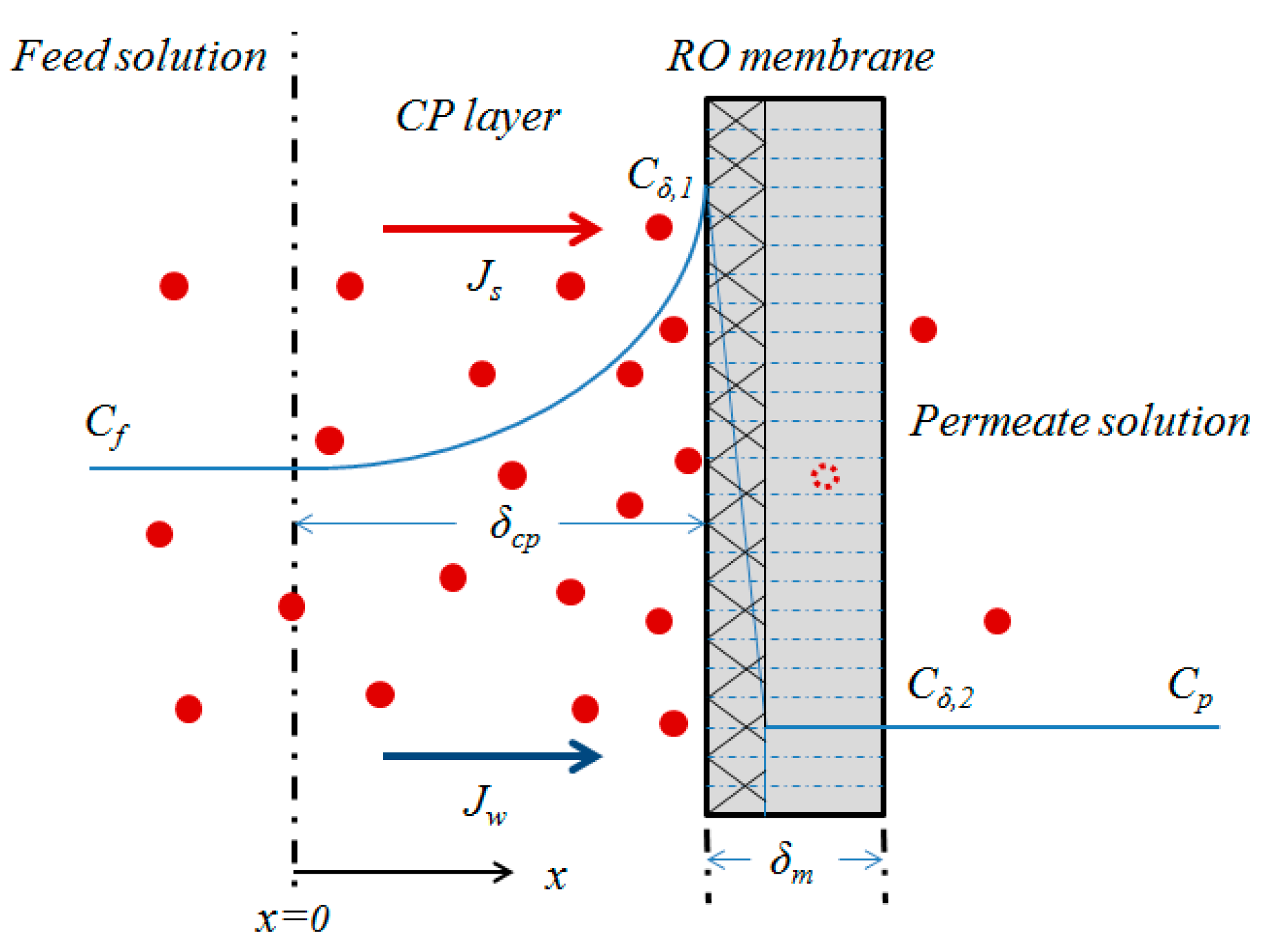
2. Theory
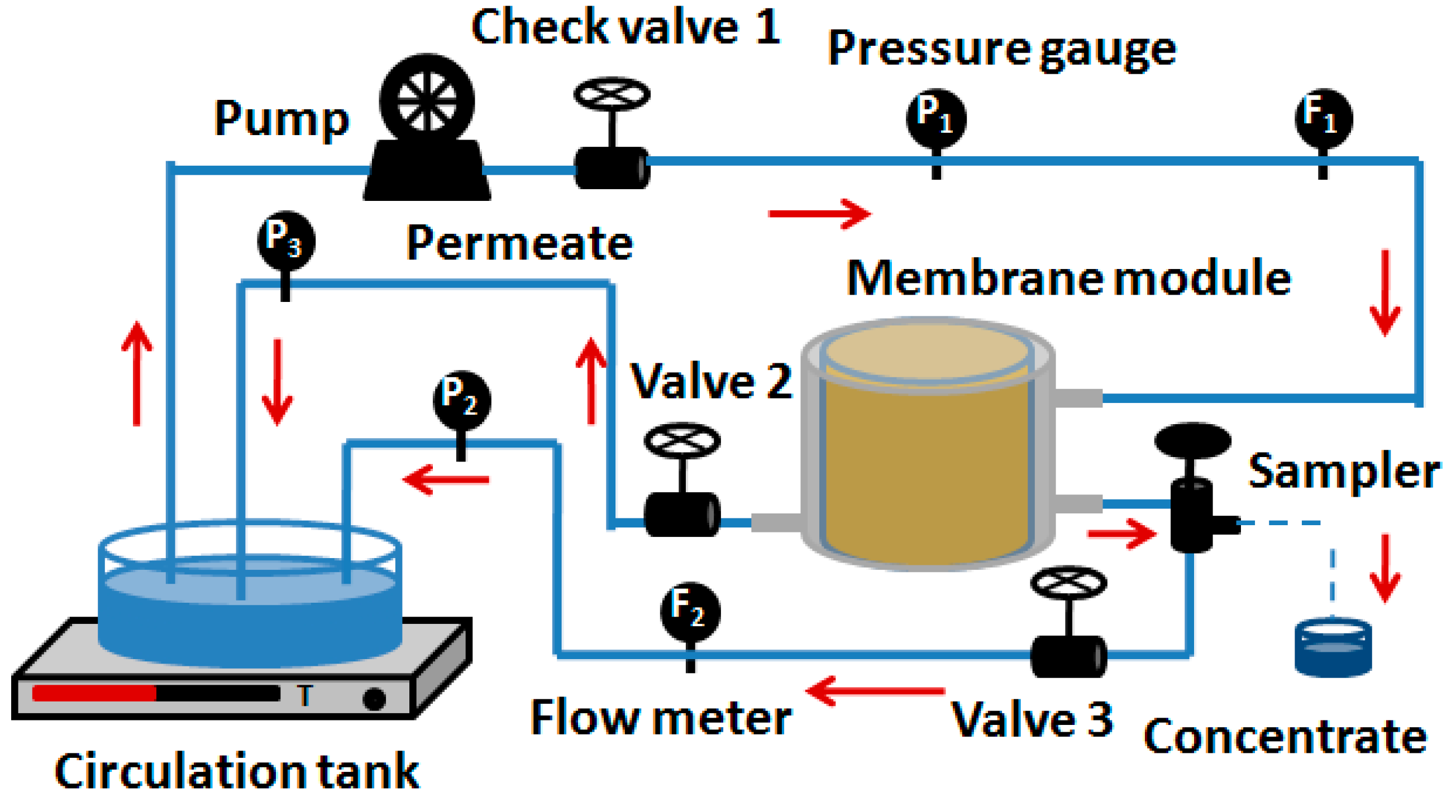
3. Experimental
3.1. Membrane and Module
3.2. Preparation of Model Solutions and Concentration Experiment
4. Results and Discussion
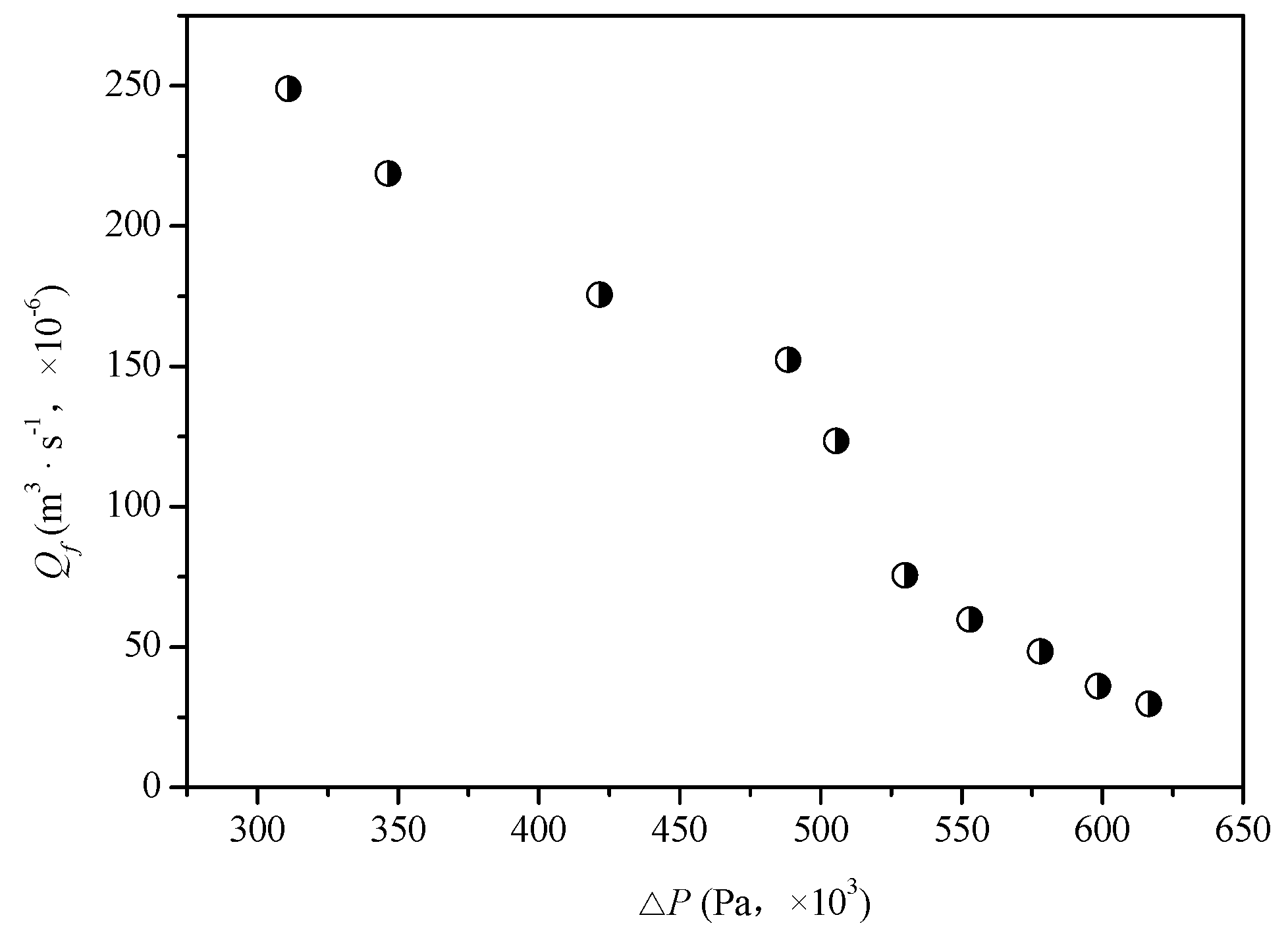
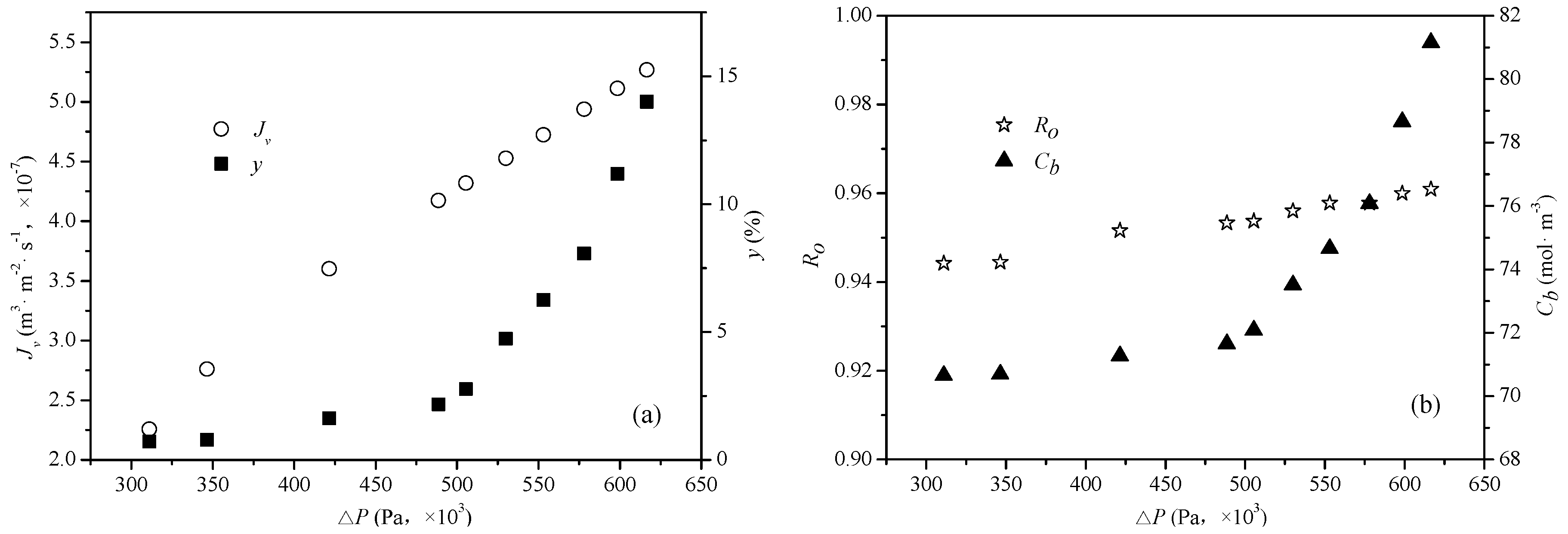
4.1. Influence of Experimental Parameters of the Reverse Osmosis System
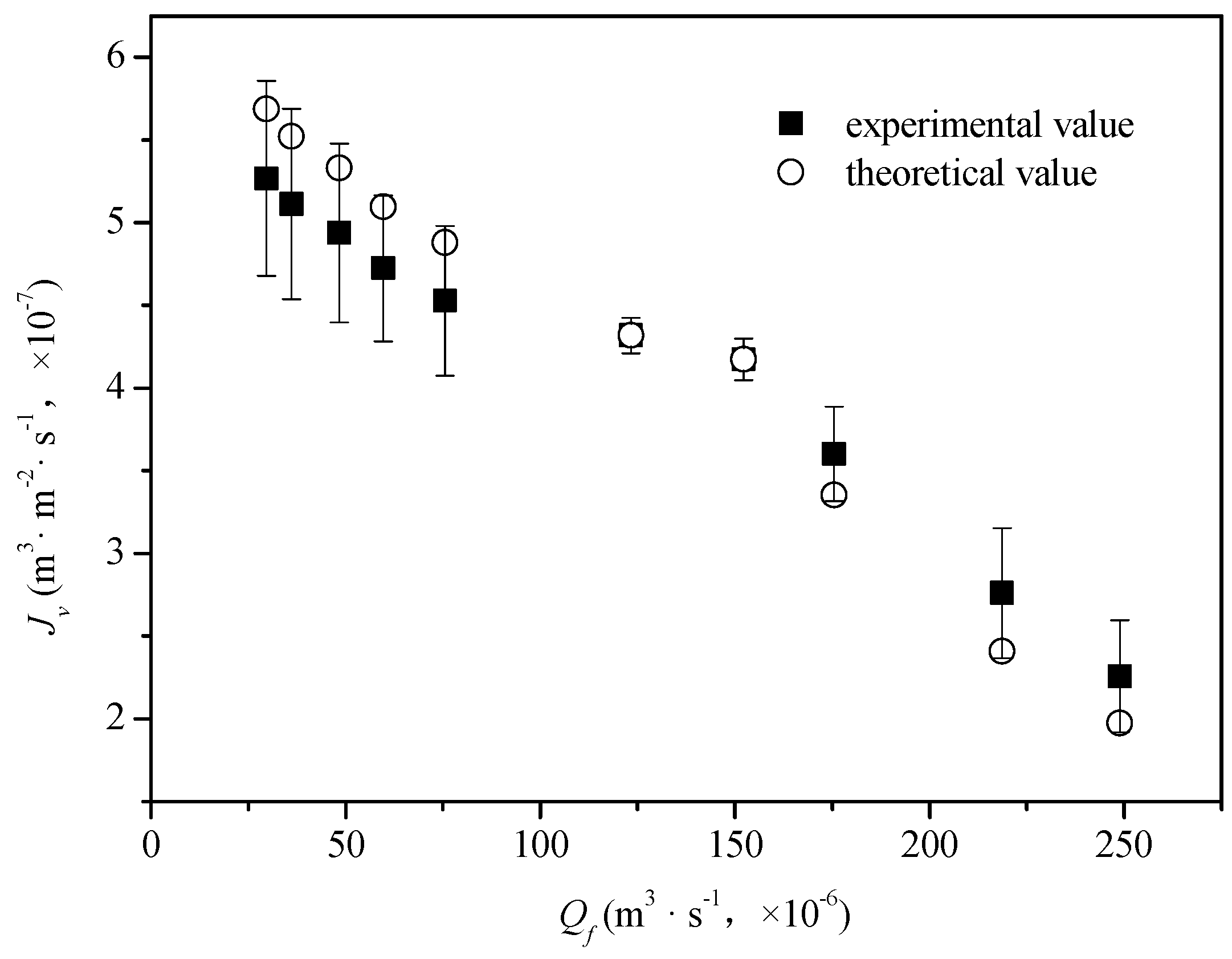
4.2. Model Validation
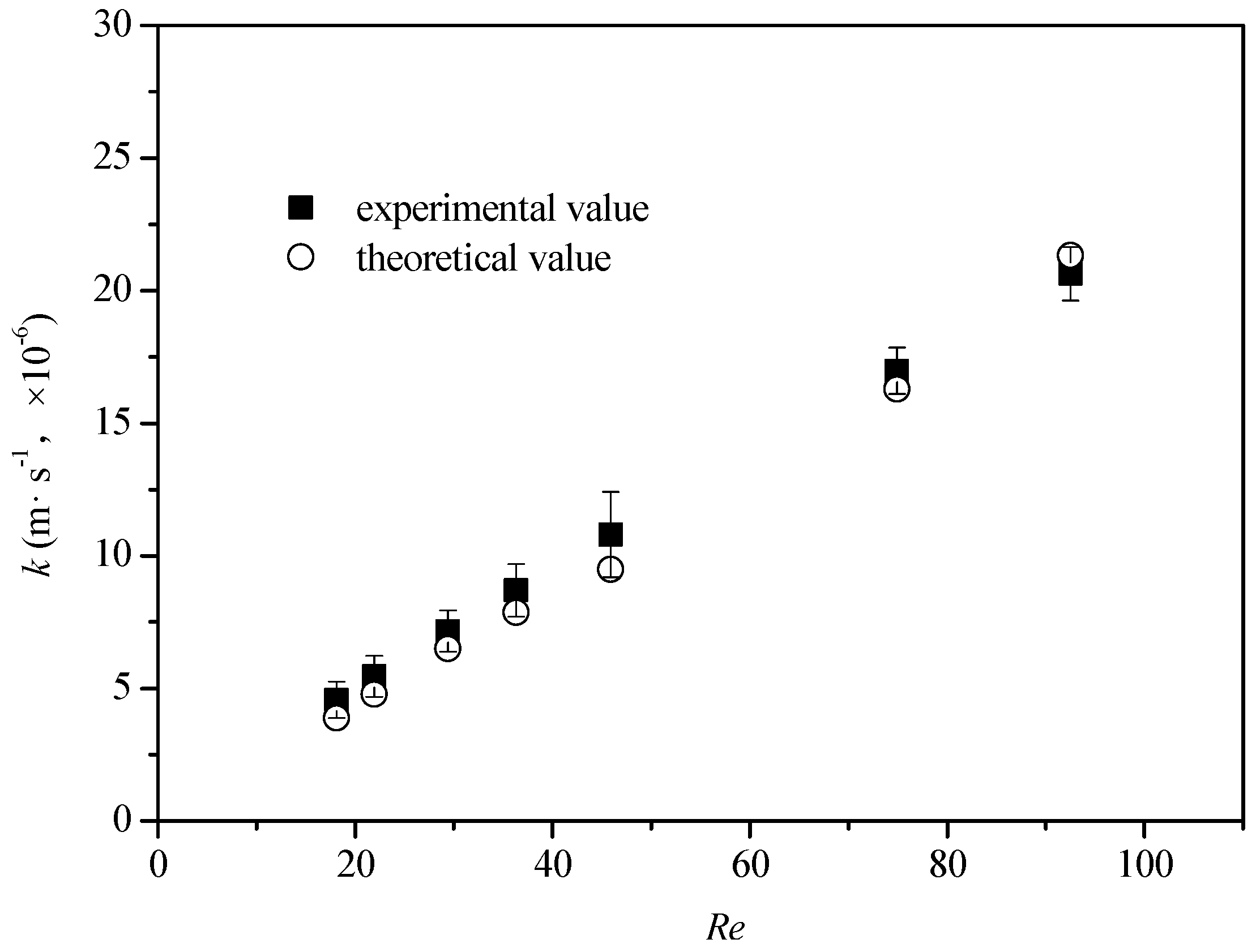
4.3. Estimation of the Mass Transfer Coefficient, k
5. Conclusions
Author Contributions
Funding
Acknowledgments
Conflicts of Interest
References
- Atab, M.S.; Smallbone, A.J.; Roskilly, A.P. A hybrid reverse osmosis/adsorption desalination plant for irrigation and drinking water. Desalination 2018, 444, 44–52. [Google Scholar] [CrossRef]
- Chung, T.S.; Zhang, S.; Wang, K.Y.; Su, J.; Ling, M.M. Forward osmosis processes: Yesterday, today and tomorrow. Desalination 2012, 287, 78–81. [Google Scholar] [CrossRef]
- Ray, S.S.; Chen, S.S.; Sangeetha, D.; Chang, H.M.; Thanh, C.N.D.; Le, Q.H.; Ku, H.M. Developments in forward osmosis and membrane distillation for desalination of waters. Environ. Chem. Lett. 2018, 16, 1247–1265. [Google Scholar] [CrossRef]
- Ray, S.S.; Chen, S.S.; Nguyen, N.C.; Nguyen, H.T.; Dan, N.P.; Thanh, B.X. Exploration of polyelectrolyte incorporated with Triton-X 114 surfactant based osmotic agent for forward osmosis desalination. J. Environ. Manag. 2018, 209, 346–353. [Google Scholar] [CrossRef] [PubMed]
- Zhou, F.; Wang, C.; Wei, J. Separation of acetic acid from monosaccharides by NF and RO membranes: Performance comparison. J. Membr. Sci. 2013, 429, 243–251. [Google Scholar] [CrossRef]
- Sundaramoorthy, S.; Srinivasan, G.; Murthy, D.V.R. An analytical model for spiral wound reverse osmosis membrane modules: Part I—Model development and parameter estimation. Desalination 2011, 280, 403–411. [Google Scholar] [CrossRef]
- Lonsdale, H.K.; Merten, U.; Riley, R.L. Transport properties of cellulose acetate osmotic membranes. J. Appl. Polym. Sci. 1965, 9, 1341–1362. [Google Scholar] [CrossRef]
- Merdaw, A.A.; Sharif, A.O.; Derwish, G.A.W. Water permeability in polymeric membranes, Part II. Desalination 2010, 257, 184–194. [Google Scholar] [CrossRef]
- Soltanieh, M.; GILL’, W.N. Review of reverse osmosis membranes and transport models. Chem. Eng. Commun. 1981, 12, 279–363. [Google Scholar] [CrossRef]
- Goosen, M.F.A.; Sablani, S.; Cin, M.D.; Wilf, M. Effect of cyclic changes in temperature and pressure on permeation properties of composite polyamide seawater reverse osmosis membranes. Sep. Sci. Technol. 2010, 46, 14–26. [Google Scholar] [CrossRef]
- Ghernaout, D. Reverse osmosis process membranes modeling—A historical overview. J. Civ. Constr. Environ. Eng. Civ. 2017, 2, 112–122. [Google Scholar]
- Qiu, T.Y.; Davies, P.A. Concentration polarization model of spiral-wound membrane modules with application to batch-mode RO desalination of brackish water. Desalination 2015, 368, 36–47. [Google Scholar] [CrossRef]
- Kim, D.Y.; Lee, M.H.; Gu, B.; Kim, J.H.; Lee, S.; Yang, D.R. Modeling of solute transport in multi-component solution for reverse osmosis membranes. Desalin. Water Treat. 2010, 15, 20–28. [Google Scholar] [CrossRef]
- Khanarmuei, M.; Ahmadisedigh, H.; Ebrahimi, I.; Gosselin, L.; Mokhtari, H. Comparative design of plug and recirculation RO systems; thermoeconomic: Case study. Energy 2017, 121, 205–219. [Google Scholar] [CrossRef]
- Spiegler, K.S.; Kedem, O. Thermodynamics of hyperfiltration (reverse osmosis): Criteria for efficient membranes. Desalination 1966, 1, 311–326. [Google Scholar] [CrossRef]
- Jain, S.; Gupta, S.K. Analysis of modified surface force pore flow model with concentration polarization and comparison with Spiegler–Kedem model in reverse osmosis systems. J. Membr. Sci. 2004, 232, 45–62. [Google Scholar] [CrossRef]
- Murthy, Z.V.P.; Chaudhari, L.B. Separation of binary heavy metals from aqueous solutions by nanofiltration and characterization of the membrane using Spiegler–Kedem model. Chem. Eng. J. 2009, 150, 181–187. [Google Scholar] [CrossRef]
- Attarde, D.; Jain, M.; Gupta, S.K. Modeling of a forward osmosis and a pressure-retarded osmosis spiral wound module using the Spiegler-Kedem model and experimental validation. Sep. Purif. Technol. 2016, 164, 182–197. [Google Scholar] [CrossRef]
- Hidalgo, A.M.; León, G.; Gómez, M.; Murcia, M.D.; Gómez, E.; Gómez, J.L. Application of the Spiegler–Kedem–Kachalsky model to the removal of 4-chlorophenol by different nanofiltration membranes. Desalination 2013, 315, 70–75. [Google Scholar] [CrossRef]
- Ahmad, A.L.; Chong, M.F.; Bhatia, S. Mathematical modeling of multiple solutes system for reverse osmosis process in palm oil mill effluent (POME) treatment. Chem. Eng. J. 2007, 132, 183–193. [Google Scholar] [CrossRef]
- Al-Bastaki, N. Removal of methyl orange dye and Na2SO4 salt from synthetic waste water using reverse osmosis. Chem. Eng. Process. Process Intensif. 2004, 43, 1561–1567. [Google Scholar] [CrossRef]
- Pastagia, K.M.; Chakraborty, S.; DasGupta, S.; Basu, J.K.; De, S. Prediction of permeate flux and concentration of two-component dye mixture in batch nanofiltration. J. Membr. Sci. 2003, 218, 195–210. [Google Scholar] [CrossRef]
- Jamal, K.; Khan, M.A.; Kamil, M. Mathematical modeling of reverse osmosis systems. Desalination 2004, 160, 29–42. [Google Scholar] [CrossRef]
- Ślȩzak, A. Irreversible thermodynamic model equations of the transport across a horizontally mounted membrane. Biophys. Chem. 1989, 34, 91–102. [Google Scholar] [CrossRef]
- Van Gauwbergen, D.; Baeyens, J. Modelling reverse osmosis by irreversible thermodynamics. Sep. Purif. Technol. 1998, 13, 117–128. [Google Scholar] [CrossRef]
- Sablani, S.S.; Goosen, M.F.A.; Al-Belushi, R.; Wilf, M. Concentration polarization in ultrafiltration and reverse osmosis: A critical review. Desalination 2001, 141, 269–289. [Google Scholar] [CrossRef]
- Gupta, V.K.; Hwang, S.T.; Krantz, W.B.; Greenberg, A.R. Characterization of nanofiltration and reverse osmosis membrane performance for aqueous salt solutions using irreversible thermodynamics. Desalination 2007, 208, 1–18. [Google Scholar] [CrossRef]
- Marquardt, D.W. An algorithm for least-squares estimation of nonlinear parameters. J. Soc. Ind. Appl. Math. 1963, 11, 431–441. [Google Scholar] [CrossRef]
- Mendes, P.; Kell, D. Non-linear optimization of biochemical pathways: Applications to metabolic engineering and parameter estimation. Bioinformatics 1998, 14, 869–883. [Google Scholar] [CrossRef]
- Dong, J.; Lu, K.; Xue, J.; Dai, S.; Zhai, R.; Pan, W. Accelerated nonrigid image registration using improved Levenberg–Marquardt method. Inf. Sci. 2018, 423, 66–79. [Google Scholar] [CrossRef]
- Zhao, C.; Ma, P.; Zhu, C.; Chen, M. Measurement and correlation on diffusion coefficients of aqueous glucose solutions. J. Chem. Ind. Eng. 2005, 56, 1–5. [Google Scholar]


| Type | PA2-4040 | |
|---|---|---|
| Membrane properties | Composition | polyamide |
| Permeable capacity (average, m3·d−1) | 7.2 | |
| Effective membrane area (m2) | 7.9 | |
| Recovery rate (single, %) | 15 | |
| Usage conditions | Maximum pressure (Mpa) | 4.14 |
| Temperature (°C) | 5–45 | |
| Maximum flow (m3·h−1) | 3.6 |
| Qf | △p | Cp | Cδ,1 | Lp |
|---|---|---|---|---|
| (m3·s−1, ×10−6) | (Pa, ×103) | (mol·m−3) | (mol·m−3) | (m·s−1·Pa−1, ×10−12) |
| 248.8889 | 311 | 3.9142 | 70.57104 | 1.3923 |
| 218.6111 | 346.5 | 3.8976 | 70.72304 | 1.3611 |
| 175.5556 | 421.5 | 3.3972 | 71.06723 | 1.3423 |
| 152.2222 | 488.5 | 3.2748 | 71.49108 | 1.3238 |
| 123.3333 | 505.5 | 3.2471 | 71.97543 | 1.3048 |
| 75.5556 | 530 | 3.0858 | 73.44194 | 1.3889 |
| 59.7222 | 553 | 2.9635 | 74.33926 | 1.3709 |
| 48.3333 | 578 | 2.9635 | 75.48901 | 1.3538 |
| 36.1111 | 598.5 | 2.8078 | 77.80078 | 1.353 |
| 29.7222 | 616.5 | 2.7411 | 79.9817 | 1.3529 |
| Qf (m3·s−1, ×10−6) | k (m·s−1, ×10−6) | dh (m, ×10−4) | Re | Sc |
|---|---|---|---|---|
| 248.8889 | 37.6 | 1.4224 | 151.2 | 482 |
| 218.6111 | 33.61 | 1.4224 | 132.8 | 482 |
| 175.5556 | 27.15 | 1.4224 | 106.6 | 482 |
| 152.2222 | 21.33 | 1.4224 | 92.5 | 482 |
| 123.3333 | 16.29 | 1.4224 | 74.9 | 482 |
| 75.5556 | 9.49 | 1.4224 | 45.9 | 482 |
| 59.7222 | 7.86 | 1.4224 | 36.3 | 482 |
| 48.3333 | 6.49 | 1.4224 | 29.4 | 482 |
| 36.1111 | 4.77 | 1.4224 | 21.9 | 482 |
| 29.7222 | 3.88 | 1.4224 | 18.1 | 482 |
| Cf (mol·m−3) | k (m·s−1, ×10−6) | Sc | D/dh (m·s−1, ×10−6) |
|---|---|---|---|
| 36.1567 | 22.2 | 484 | 1.1710 |
| 62.4444 | 21.95 | 482 | 1.1703 |
| 87.5533 | 21.77 | 480 | 1.1696 |
| 111.506 | 21.6 | 479 | 1.1689 |
| 137.149 | 21.4 | 478 | 1.1682 |
© 2019 by the authors. Licensee MDPI, Basel, Switzerland. This article is an open access article distributed under the terms and conditions of the Creative Commons Attribution (CC BY) license (http://creativecommons.org/licenses/by/4.0/).
Share and Cite
Chen, C.; Qin, H. A Mathematical Modeling of the Reverse Osmosis Concentration Process of a Glucose Solution. Processes 2019, 7, 271. https://doi.org/10.3390/pr7050271
Chen C, Qin H. A Mathematical Modeling of the Reverse Osmosis Concentration Process of a Glucose Solution. Processes. 2019; 7(5):271. https://doi.org/10.3390/pr7050271
Chicago/Turabian StyleChen, Chenghan, and Han Qin. 2019. "A Mathematical Modeling of the Reverse Osmosis Concentration Process of a Glucose Solution" Processes 7, no. 5: 271. https://doi.org/10.3390/pr7050271
APA StyleChen, C., & Qin, H. (2019). A Mathematical Modeling of the Reverse Osmosis Concentration Process of a Glucose Solution. Processes, 7(5), 271. https://doi.org/10.3390/pr7050271