The Effects of Water Friction Loss Calculation on the Thermal Field of the Canned Motor

Abstract

The thermal behavior of a canned motor also depends on the losses and the cooling capability, and these losses cause an increase in the temperature of the stator winding. This paper focuses on the modeling and simulation of the thermal fields of the large canned induction motor by different calculation methods of water friction loss. The values of water friction losses are set as heat sources in the corresponding clearance of water at different positions along the duct and are calculated by the analytical method, loss separation test method, and by assuming the values that may be larger than the experimental results and at zero. Based on Finite volume method (FVM), 3D turbulent flow and heat transfer equations of the canned motor are solve numerically to obtain the temperature distributions of different parts of the motor. The analysis results of water friction loss are compared with the measurements, obtained from the total losses using the loss separation method. The results show that the magnitude of water friction loss within various parts of the motor does not affect the position of peak temperature and the tendency of the temperature distribution of windings. This paper is highly significant for the design of cooling structures of electrical machines.

1. Introduction

The canned motors are currently limited by bearing technologies and the thermal field, preventing a high reliability and long lifetime. The thermal behavior of electric machines can be determined by losses and cooling capability [1,2]. Generally, the losses can be divided into water friction loss, electric loss, including rotor and stator shield loss, stator winding loss, rotor copper bar loss, conical ring loss, iron loss, and eddy-current loss. Electric loss and eddy-current loss can be obtained by the finite element method (FEM) [3]. Due to the characteristics of high thermal density per unit volume of rotor and stator shield and small water clearance in the shield, the water friction loss distribution in canned motors differs from conventional standard motors. The most temperature-sensitive component of the motor is the radial bearings, and their operating temperature should be lower than the alarm value. The effects of losses on the temperature rise of the motor components, such as stator windings, insulations, and radial bearings, is a very important issue [4,5]. Water friction loss calculation methods and thermal analysis, thus, are an important step in the designing of induction motors. Moreover, temperature variations also affect the circulation of cooling fluids and their flow dynamics [6].

Typically, thermal analysis can be carried out using computational fluid dynamics (CFD) [6,7,8], the heat equation finite element analysis (FEA) [4], or lumped parameter thermal network (LPTN) models [9,10,11], and the first two are very accurate and deliver proper predictions of the thermal system behavior during the component/device development. Finite volume method (FVM) is one of the CFD methods and has the advantage of predicting the flow in complex regions and obtaining the temperature distribution [8].

With the development of high speed motors and their applications, the research and study of the effect of different losses of motors have become topics of high interest. Luomi et al. [12] studied and proposed a method for loss minimization including air-friction losses and explained that the design is considerably influenced by the air-friction losses, resulting in a small diameter of the rotor. Wang et al. [13] analyzed rotor losses of permanent magnet synchronous machine (PMSM) with experiments and simulations and focused on rotor loss in the no load running condition. Aglen and Andersson [14] theoretically and experimentally studied and calculated different losses of the generator. They utilized a generator model to inspect the temperature distribution and showed that different losses strongly affect the temperature distribution, particularly the temperature of the magnet due to rotor losses. Leakage effects while proposing a design method for bearing were studied by Le Yun et al. [15]. They discussed the effect of leakages in terms of static and dynamic stiffness. Zhang and Kirtely et al. [16] investigated and predicted the power losses including core losses, winding losses, and air-friction losses. The effects of friction loss in electric machines were often neglected in past research; however, in recent years, the friction loss has been considered one of the important factors that might affect the bearing life of the canned motor and account for the percentage of fly wheel loss of the motor due to the increased rotational speeds. As in [12], a method for efficiency optimization of a 500,000-r/min permanent magnet machine has been studied.

There is no study on the friction loss and calculation method of the water-cooled canned motor for the temperature rise of internal components and bearing safety. When the electric loss of the motor is constant, the magnitude and calculation method of friction loss have an influence on the peak temperature of the winding. The research object is a canned motor in this paper; a calculation method is presented to study the effect of friction losses on the thermal field of the motor, and the effect on the peak temperature and temperature variation characteristics of important parts are analyzed. The study has been carried out by computational fluid dynamics (CFD) approaches adopting five friction loss values: theoretical, experimental, assumed 1.1-times experimental, and the CFD module; the last one is the ideal case assuming no friction loss.

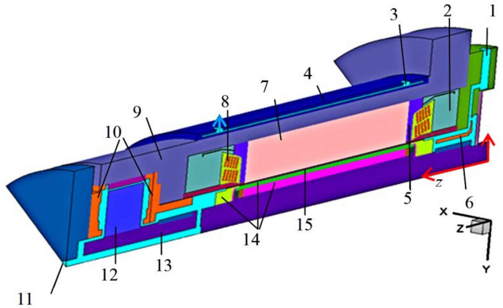
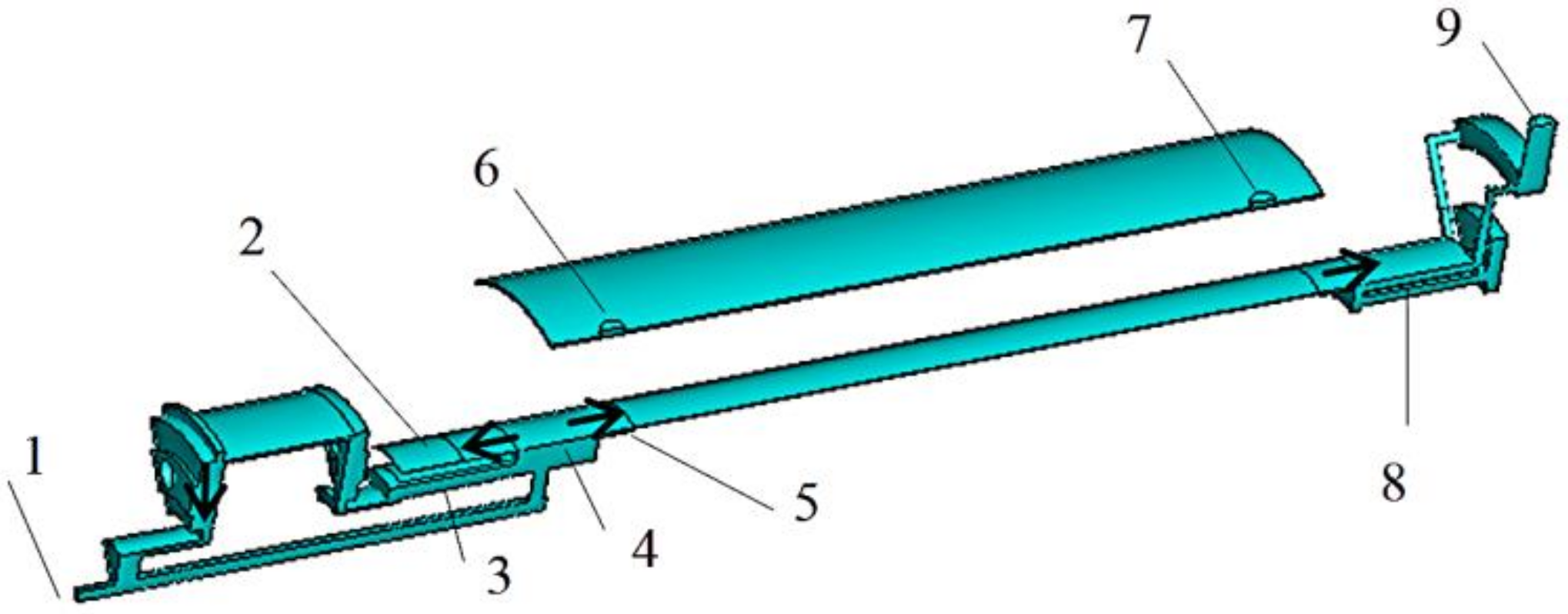
2. Physical Model

The studied electrical machine was a vertical squirrel cage motor with a rotational speed of 1500 r/min, 6600 kW (see Figure 1). It had a three-phase, four-pole, short-pitched, and double-layer winding stator whose outside diameter was 1.3 m. The air gap clearance was 4.2 mm; the thickness of the stator and rotor shield casing was 0.46 mm and 0.70 mm, respectively, and the dimensionless ratio between core length and rotor inside diameter was 6.5. It had N-class insulation of the winding with a permitted temperature of 200 °C.

In Figure 1, 1 indicates the outlet, 2 the upper nitrogen end room, 3 the water inlet, 4 the cooling jacket, 5 the stator plate, 6 the upper radial bearing, 7 the stator core, 8 the winding end, 9 the frame, 10 the lower radial bearing, 11 the primary water inlet, 12 the lower fly wheel, 13 the axis, 14 the cage rotor, and 15 the stator can.

The temperature of each part can be reduced by the effective internal and external circuit design of the primary cooling water. The secondary cooling water flowed from the upper part of the outer casing (bottom outflow); see Figure 2. The primary water flowing out of the external heat exchanger was drawn through the axial suction hole at the bottom of the frame. Water continued to flow upward to the auxiliary impeller position and was thrown away by the Coriolis force. A part of the cooling water flowed down for the cooling and lubrication of the lower guide bearing and lower fly wheel, then entered into the cycle of cold water confluence and moved downward.

Considering the continuity of flow of water in the shield, the geometry characteristics of rotor and stator winding slots along the circumference, and the characteristics of heat transfer in stator and rotor material, the 1/8th structure of the motor along circumferential direction was simulated. The rotor shaft of the model was coincident with the z-coordinates; the positive direction of z-axis was towards down, and the y-axis was positive along radial direction. The coordinate origin point was located in the upper part and can be seen in Figure 1.

In Figure 2, 1 indicates the primary water Inlet, 2 the flywheel clearance inert zone, 3 the lower radial bearing clearance, 4 the auxiliary impeller position (confluence region), 5 the water in double cans clearance, 6 the secondary water exit, 7 the secondary water inlet, 8 the upper radial bearing clearance, and 9 the primary water outlet.

3. Solution Conditions

3.1. Basic Assumptions

• The water in the motor was an incompressible fluid because the Mach number (Ma = 0.24) was far less than 0.7. The mass flow rate (5.127 kg/s) of primary water was very large in the clearance of the motor. The Reynolds’s number (Re = 5363) showed that the flow was in the turbulence state.
• Only the steady state of fluid flow was considered. There was no contact thermal resistance between the adjacent bodies. The flow of the fluid in the internal passage was in the smooth region because the internal surface roughness of the wall in the motor was very small and the friction loss can be uniformly implemented for the corresponding positions of the water as volumetric heat sources inside the fluid.
• The electrical and harmonic losses and their distribution were calculated by another research institute using 3D software from the electromagnetic field. The corresponding loss in each body was uniformly distributed. Because the parameters of the thermo-physical properties of materials change with temperature variations, e.g., thermal conductivity, density, and specific heat at constant pressure, to be on the safe side, they were set as constant in the calculation process, so the minimum value of these parameters was chosen in the interval of the temperature through a large number of calculations. Among them, the thermal conductivity of the iron core lamination of rotor and stator was anisotropic, and the axial, radial, and tangential values of thermal conductivity were chosen experimentally. Except iron core lamination, other materials were isotropic, and their thermal conductivity values were selected conventionally.

3.2. Mathematical Model

The rotation of the water in the shield sleeve gap and the water in the center of the axis was considered in the calculation process because the rotor rotated rapidly relative to the stator under the condition of stable operation. Therefore, a multiple reference-frame system and the rotational speed of the wall surface were selected in the Ansys Fluent software (v14.5, Fluent Inc., New York, NY, USA, 2012). Three-dimensional flow and heat transfer coupling equations including the mass and momentum conservation equation and the relation of absolute velocity vector u (the velocity viewed from the stationary frame) and relative velocity vector u_r (the velocity viewed from the rotating frame) can be written as follows:

$$\nabla \left(\rho u_r\right)$$

(1)

$$\nabla \left(\rho u_r{u}_r\right)+\rho \left(2\Omega \times u_r+\Omega \times \Omega \times r\right)=-\nabla p+\nabla \tau +F)$$

(2)

$$u=u_r+\Omega \times r$$

(3)

In the fixed reference frame, mass, momentum, and energy conservation equations can be replaced by a general control equation, which is given in Equation (4).

$$\nabla \left(\rho u\varnothing \right)=\nabla \left(\mathsf{\Gamma }grad\varphi \right)+S$$

(4)

where Ω is the angular velocity of the rotor, ɸ is a universal variable, which can be replaced by unknown variables u, v, w, T, etc., Γ is the generalized diffusion coefficient, and S is the generalized source term. The only difference among the variables was the setting condition of Γ, S, initial values, and boundary conditions. The specific expressions of Γ, S for different variables were provided in [16]. In addition, for the solid components in the motor, the energy equation was converted into the heat conduction differential equation due to the no convection item. In the shielded motor, the mode of heat transfer was conduction between and inside the solid materials (e.g., stator core), and between the solid and liquid was the convection heat transfer. The natural convective heat transfer occurred between the nitrogen and the adjacent solid wall surfaces at the end of the wire rod in the upper and lower end closed room, and the magnitude of natural convection heat transfer was determined by the temperature or density difference. The flow of water in the shielded casing and outer casing was a mixed flow, and the natural convection in these regions can be neglected. Due to the small clearance between the stator and rotor shield sleeve and in the three bearings, the width of flow was in the order of millimeters. The forced convection flow in this region was affected by viscous shear stress and Coriolis force, an effect whereby a mass moving in a rotation system experiences a force acting perpendicular to the direction of motion and to the axis of rotation. Since a forced convection flow around a cylinder is dominated by viscous shear forces in the boundary layer and the velocity gradient between the walls is very large, so, in this paper, the shear stress transport (SST) k-ω two-equation mathematical model was adopted. This model included two transport equations to represent the turbulent properties of the flow. The first transported variable was turbulent kinetic energy k, and the second transported variable was ω. These transported variables determined the energy in turbulence and the scale of turbulence, respectively, and their equations can be written as follows:

$$\frac{\partial }{\partial x_i}\left(\rho k{u}_i\right)=\frac{\partial }{\partial x_j}\left({\mathsf{\Gamma }}_k\frac{\partial k}{\partial x_j}\right)+G_k-Y_k+S_k$$

(5)

$$\frac{\partial }{\partial x_i}\left(\rho \omega u_i\right)=\frac{\partial }{\partial x_j}\left({\mathsf{\Gamma }}_{\omega }\frac{\partial \omega }{\partial x_j}\right)+G_{\omega }-Y_{\omega }+S_{\omega }+D_{\omega }$$

(6)

In the above equations, G_k and G_ω represent the generation of k and ω due to mean velocity gradients. Γ_k and Γ_ω represent the effective diffusivity of k and ω, respectively. Y_k and Y_ω represent the dissipation of k and ω due to turbulence. D_ω represents the cross-diffusion term. S_k and S_ω are user-defined source terms [17].

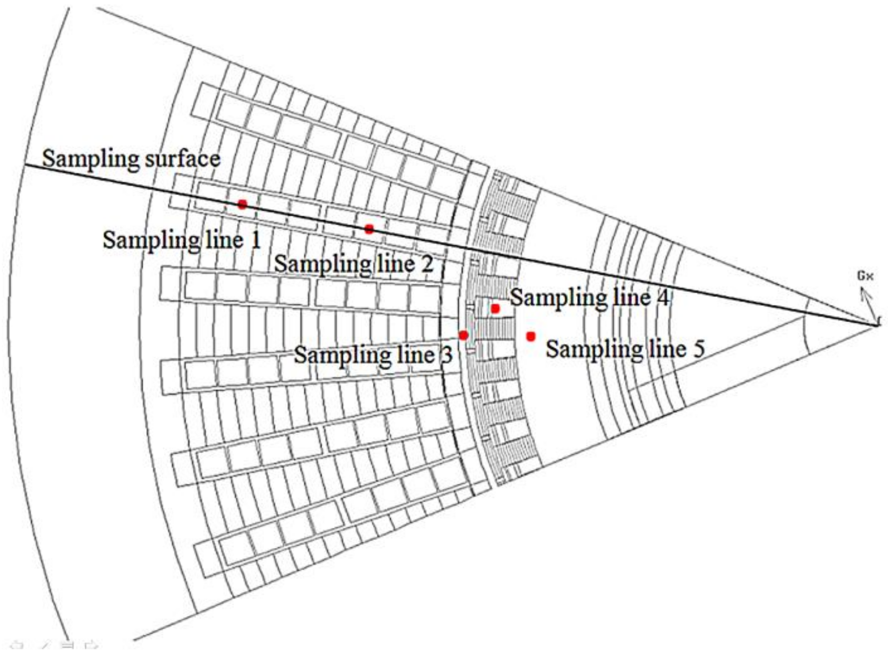
3.3. Mesh Generation

Due to the complex geometry of the model, both structured and unstructured meshes were used, while the total number of cells was 14,099,447, and the value of equisized skew was less than 0.8 for the overall mesh. The mesh was refined into those regions where large velocity and pressure gradients were expected. In this paper, the grid independence solution was obtained after employing different meshing schemes, interval sizes, and calculations.

3.4. Loss and Boundary Conditions

3.4.1. Water Friction Loss

There were losses that caused the temperature rise in the motor, and in this paper, only water friction loss and relative influencing factors were given more attention. Principally, friction loss can be divided into loss along the path and local losses. The losses along the path were due to the frictional resistance caused by the fluid moving along the flow path and occurred in the fluid boundary layer where the velocity gradient was comparatively large. Local losses were due to fluid flow through various curved pipelines, for example, in elbows, valves, etc., due to the deformation of water flow, the change of direction, and speed redistribution, and the internal eddy current caused losses. The loss along the path was caused by viscous friction, and the frictional resistance coefficient was closely related to the surface roughness of the water channel, the state of flow, and the properties of the coolant.

In this paper, the value of surface roughness for each method was set the same. The analysis of friction losses in the water gap clearance can be estimated by the equation derived for rotating cylinders, which can be written as [18,19]:

$$P=k{c}_f\pi \rho {\mathsf{\Omega }}^3{r}^4$$

(7)

where k is the roughness coefficient, where the value was 1.0 for smooth surface [4], ρ is the density of water, l is the length of the cylinder, and r is the rotor radius. The friction coefficient c_f depends on the radius of the cylinder, the radial air-gap length δ, and the Reynolds number. The calculated result of the water friction loss at every clearance position of the water channel can be seen in

Table 1. Four conditions of friction losses (kW) at different positions in the water clearance region.

Clearance Position	Assumed Value	Analysis Value	Test Value	Assumed Value
Shield sleeve	0	384	407	407 × 1.1%
Upper radial bearing	0	17	17	17 × 1.1%
Lower radial bearing	0	17	17	17 × 1.1%
Upper fly wheel	0	793	722	722 × 1.1%
Lower fly wheel	0	580	690	690 × 1.1%
Auxiliary wheel	0	7	7	7 × 1.1%
Total	0	1798	1860	2046

Note: The data in the Table 1 are the sum of local and along-the-way losses at each location.

. In order to verify the accuracy of the calculation results, a friction loss experiment was also carried out. The experimental loss value was obtained by the loss-separation method [18] and was provided by the manufacturer.

Table 1 shows that the analysis value of the water friction loss in the water clearance (region) of the lower fly wheel and double cans was smaller than that of the test value by 110 kW and 23 kW, respectively, and of the upper flywheel was larger than the test value by 71 kW. Analysis of friction loss was smaller than the experimental friction loss by 62 kW, a relative difference of −3.33%; hence, the results were accurate (the total experimental friction loss was large). Based on previous experience and for the sake of operational safety, it was assumed that the actual operating condition (value) was higher than the test value by 10% in every term. The values of analysis and experimental water friction loss at each position were provided by the manufacturer; see Table 1. In order to separate the influence of water friction loss on temperature rise, a situation in which the water friction loss was assumed as zero was designed, as shown in the Table 1.

It was assumed that the friction losses at each location was evenly distributed. The value of water friction loss per unit volume as a source term (kW/m³) was calculated according to Table 1, and these values were applied to the corresponding boundary volume of water, respectively. The CFD method was different from the above-mentioned conditions in Table 1. The friction loss in the clearance of water at different positions was calculated by the CFD FLUENT software. The specific way of selecting the viscous heating item was to select it in the “options” list, which is right under the turbulence model, and the wall roughness was set in the boundary conditions according to the different positions of the cans. All the related settings and parameters used in the CFD models above calculations are listed in

Table 2. The settings and parameters in the computational fluid dynamics (CFD) models for temperature calculations. SST, shear stress transport.

	CFD	Assumed	Analysis	Test	Assumed Value
Models-viscous-(SST) k-ω	on	on	on	on	on
Models-energy	on	on	on	on	on
Options-viscous heating	on	off	off	off	off
Boundary condition-moving wall	set	-	-	-	-
Shear condition	no slip	-	-	-	-
Wall roughness (mm)	1.0	-	-	-	-
Source item in water clearance region (kW/m3)	-	-	on	on	on

Note: “-” denotes no need to set any value.

. We can see the differences between the two calculation methods of water fiction loss.

3.4.2. Electrical Loss

The electric loss in the rotor was calculated in the iron core, the shield sleeve, the end of the coupling loop, and in the copper bar. Harmonic loss of the wire rod was also a part of this calculation. The electric loss in stator was calculated in the shield sleeve, the copper bar, and in the iron core. In particular, the stator and rotor core teeth and yoke loss were calculated separately, and the teeth were divided into 16 sections along the radial direction. In addition, the loss value of the conical ring, teeth, and yoke position of the stator finger plate was considered. The stray loss was calculated by the experimental formula developed by the factory for the same kind of shield motor. By using the same loss calculation method as used in [3], the obtained calculated values of the main parts were as given in

Table 3. Electrical loss values in the main solid components.

Components	Loss (kW)
Rotor copper bar	72.0
Rotor shield (casing)	262.57
Stator winding	44.54
Stator shield (casing)	920.58
Conical ring	28.53
Rotor copper bar	72.0
Rotor shield (casing)	262.57
Stator winding	44.54
Stator shield (casing)	920.58
Conical ring	28.53

.

It can be noted from the above table that the electrical loss was comparatively more in the rotor and stator shielding case. It was assumed that all electrical losses were distributed uniformly in the corresponding components.

3.4.3. Boundary Conditions

The inlet boundary condition of the volume flow rate of water was mainly determined by the intersection point of the pump and motor operating curves and partially determined by the geometry characteristics. The entrance of the primary water below the base and the entrance of the external cooling water in the upper part of the shielding casing (see Figure 2) were the velocity boundary conditions, and the magnitude of velocity was set experimentally. The rated rotating speed of the motor shaft was 1500 r/min.

The inlet-outlet temperature of the primary water was closely related to factors such as the magnitude of internal friction loss, the temperature of cooling water in the external heat exchanger (same as the secondary water temperature in the cooling jacket), and the velocity of water. Through the calculation of the heat balance and heat transfer of the internal motor and external heat exchanger, respectively, and between the internal motor and external heat exchanger, at the operating condition of the highest external cooling water temperature of 41 °C at entrance, we obtained the internal cooling water inlet temperatures, 60.38 °C, 61.65 °C, and 62.99 °C, at the three mentioned conditions. For the convenience of comparison, the temperature of the internal water inlet was set at the same temperature of 60.38 °C.

The gauge pressure at the outlet of the external water was set to 0 Pa. The mode of heat transfer in the outer surface of the shell was natural convection. For safety measures, the surface convective heat transfer coefficient was set to 1 W (m² K), and the ambient air temperature of the outer surface was 48.9 °C. The boundary condition at the top of the motor was constant heat flux, and its value was water friction loss per unit volume at the bottom fluid of the flywheel. The boundary conditions of the right and left surface of the calculation domain (see Figure 1) were linked periodically. In addition, the governing equations for the fluid and solid regions were solved by using FLUENT 14.5, which uses the finite volume method. A second order upwind scheme was employed for the discretization of all the variables, and the simple scheme was used for the pressure-velocity coupling. The standard wall function was used to deal with the viscosity lamination near the solid wall surface, and the dimensionless distance y+ met the requirements. After trying several different mesh topologies and sizes, the grid-independent solution was obtained.

4. Results and Discussion

The temperature field in the solution domain was obtained by means of numerical simulation of Equations (1)–(6) at the loss and boundary conditions mentioned above.

For the convenience of analysis, five straight lines (sampling lines) parallel to the rotation axis were drawn in order to get the axial variation law of physical quantity. The position of each line is shown in Figure 3, and the number of sampling lines required for the analysis is given in decreasing order of radii. The sampling surface was located at the radial cross-section of the stator slot; Sampling Lines 1 and 2 pass through the center of the stator lower and upper winding, respectively, and the start and end coordinates of the two lines are the same. Sampling Line 3 is located in the center of the clearance of the cooling water between the stator and rotor shield, and Sampling Lines 4 and 5 pass through the center of a rotor bar and the rotor core, respectively. This paper presents the analysis of the effect of water friction loss on the temperature of canned motor components such as the stator winding, rotor copper bar, rotor iron core, and on the internal water passage. The temperature analysis of different parts is described below.

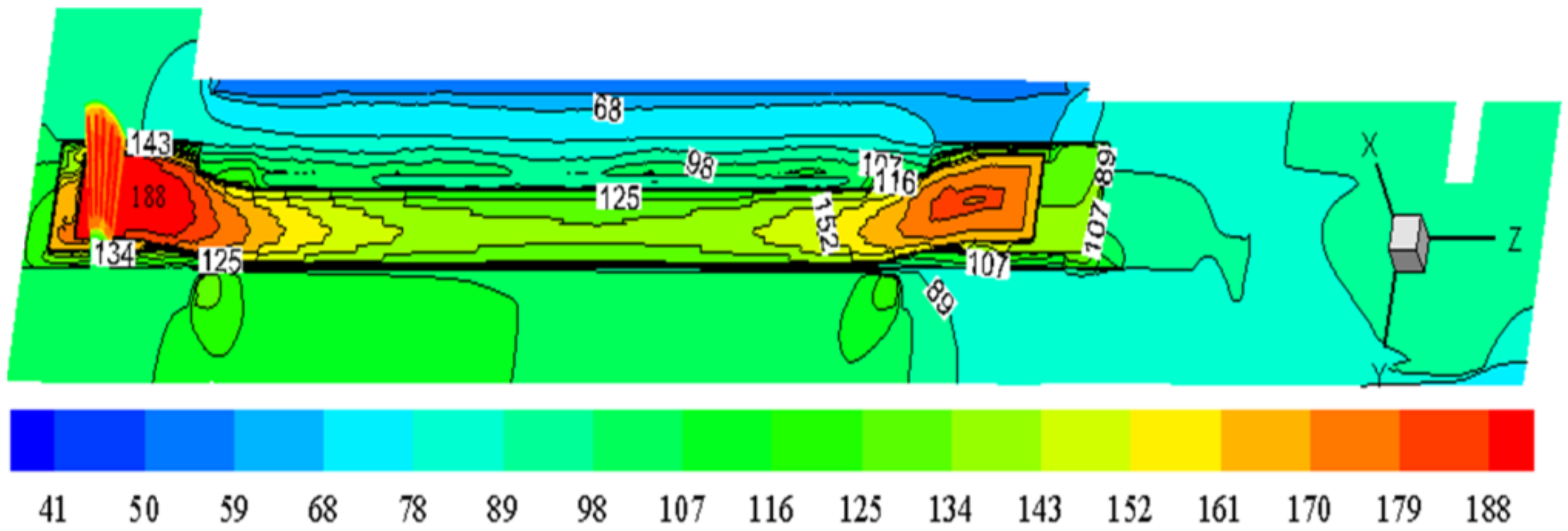
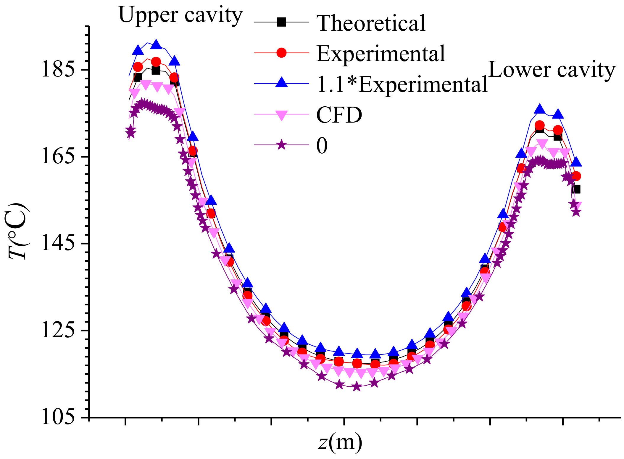
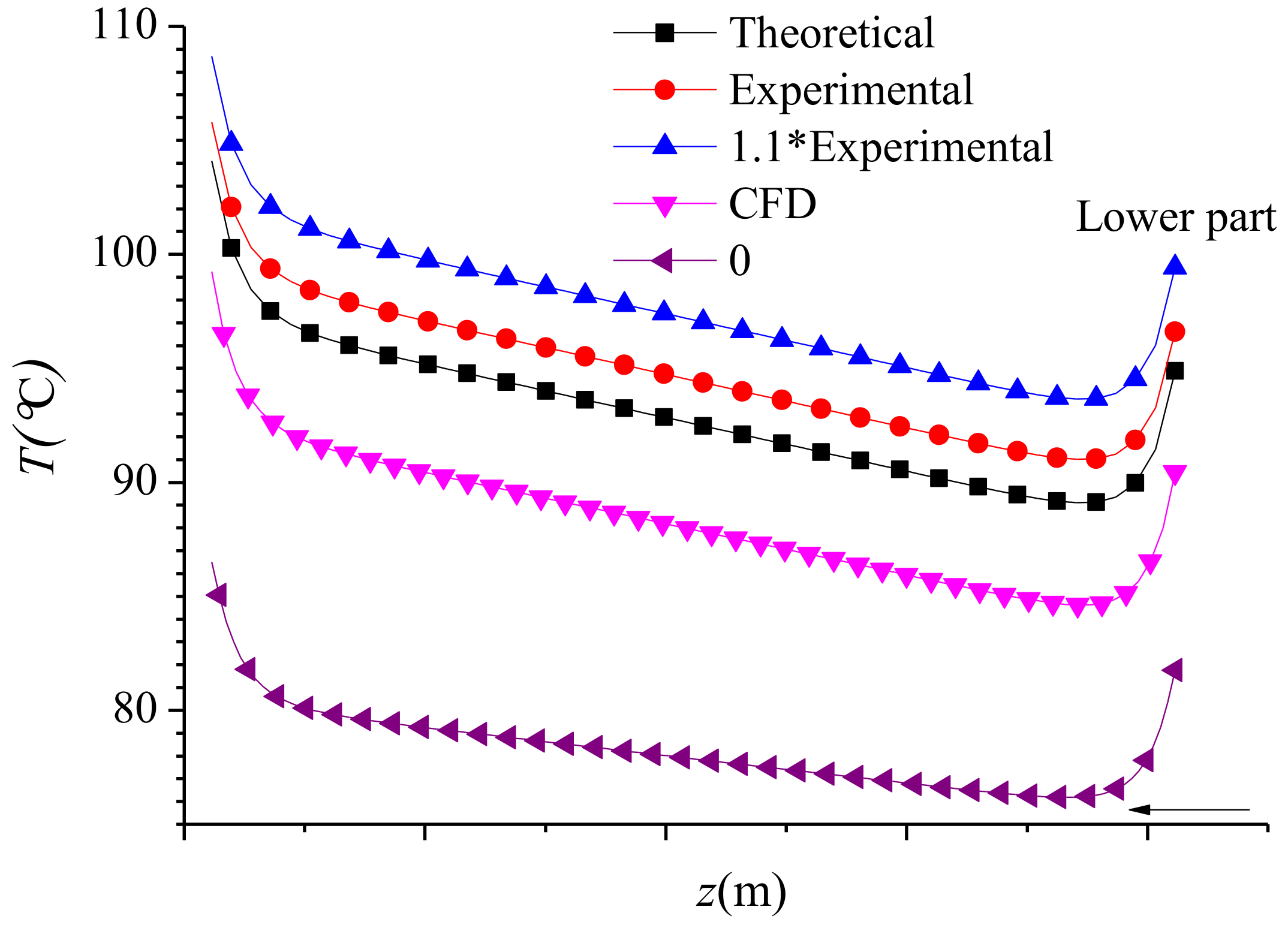
4.1. Temperature Analysis of the Stator Winding

The temperature distribution characteristics of the stator winding were the same in the axial direction, and the highest temperature point was located in the middle of the nose of the two ends of the stator winding (see Figure 4), resulting in a reduction of the heat by the conduction from the two ends of the stator to the middle, and was then delivered by the primary and secondary water convection. The position of peak temperature was not changed when calculated for four different conditions; assuming no fiction loss, analysis, experimental, and assuming 1.1-times the experimental value. The peak temperature increased gradually by 178.6 °C, 185.8 °C, 188.2 °C, and 192.0 °C, and the maximum temperature did not exceed the permitted temperature of 200 °C, i.e., no over-temperature.

The results showed that electrical loss was the main factor that rose the temperature of the winding, although the total value of the analysis of water friction loss was comparatively higher, but did not strongly affect the peak value of the temperature. Comparing it (peak temperature) with the no fiction loss condition, its temperature value increased by 7.2 °C, 9.6 °C, and 13.4 °C, and it showed that if the mechanical loss of water friction was neglected, the error would be about 10 °C. Comparing it (peak temperature) with the experimental calculation of the water friction loss condition, its temperature value increased by −2.4 °C and 3.8 °C, and the error was within the range ±2.0%, while the values of peak temperature increased non-linearly. The temperature contour of the stator winding at assumed 1.1-times the experimental calculation condition of water friction loss (maximum friction loss) is given in Figure 4.

In order to analyze the influence of water friction loss calculation methods on the temperature field of the motor, using the same conditions mentioned above and the CFD module, the obtained results showed that the peak temperature of the motor winding was 180.9 °C, and comparing with the experimental water friction loss values, it reduced by 7.93 °C (error was −3.84.2%), while temperature distribution characteristics and peak position did not change. The value of temperature was lower when calculated by the CFD module. The main cause of the error was that the actual wall roughness was higher than 1.0 mm.

It can be seen from Figure 4 that the peak temperature of the end center of the stator winding nose in the upper nitrogen end room was 192.0 °C. The highest temperature of stator winding in the lower nitrogen end room was lower than that in the upper part. The temperature of the winding adjacent to the central part of the iron core was lower because the surrounding water temperature in the internal gap and in external casing was lower and the convection heat transfer capability of the water was strong.

Figure 5 shows the temperature contour on the sampling surface for the test calculated condition. Theoretically, the temperature distribution characteristics on the surface of any polar angle along the circumferential cross-section are a typical case. The overall temperature distribution characteristics of any component along the radial direction can be seen in Figure 5. The temperature of the casing near the cooling water zones was low. Secondly, the temperature of the water in the stator and rotor shield sleeve clearance, stator iron core, and the rotor was higher; the stator winding temperature in the upper nitrogen chamber was the highest; and the temperature gradient near the tooth clamp plate was relatively large.

Figure 6 and Figure 7 show the temperature distribution of Sampling Lines 1 and 2 of the stator winding along the z-axis, respectively. From Figure 6 and Figure 7, it can be seen that the temperature distribution of the winding presented a concave curve, and the lowest temperature point in the upper and lower windings was near the axial center of the windings. Ignoring frictional losses, the temperature rise caused by electric loss was shown in the curve corresponding to “0” in the figure, and this curve can be used as a benchmark for comparison. In comparison, it can be found that the temperature rise of the winding due to frictional loss at the upper and lower ends and the intermediate position was larger. It is one of the main purposes of this paper to reveal the influence of friction loss on the calculation of peak temperature. Except for the cavity at both ends, for the theoretical and experimental friction losses, the temperature distribution curve was basically coincident.

The temperature distribution of the winding was not symmetrical along the axial center of the iron core. The temperature gradient in the left part of the winding was higher than that in the right part of the winding, and the winding temperature in the upper stator cavity was higher than that of the lower stator cavity. In the same z-coordinates, the temperature of Sampling Line 1 of the lower winding was higher than the temperature of Sampling Line 2. For Sampling Line 2, where the upper winding location was closer to the shaft, the actual length of the winding nose was short in the upper and lower part of the stator cavity.

In Figure 7, the irregular variation of the curve indicates the change of temperature in insulation, nitrogen (end room), and other parts through which the sampling line passed after stretching out the straight winding. Under conditions of analysis of and experimental water friction loss, the temperature of the winding was basically the same for the same position, except the end cavity. However, for the two end stator cavities, the calculation results were different in the five cases. The value of the winding temperature was the highest at the same position along the z-axis, under the water friction loss condition of 1.1-times the experimental value, and was lowest when calculated by the CFD module.

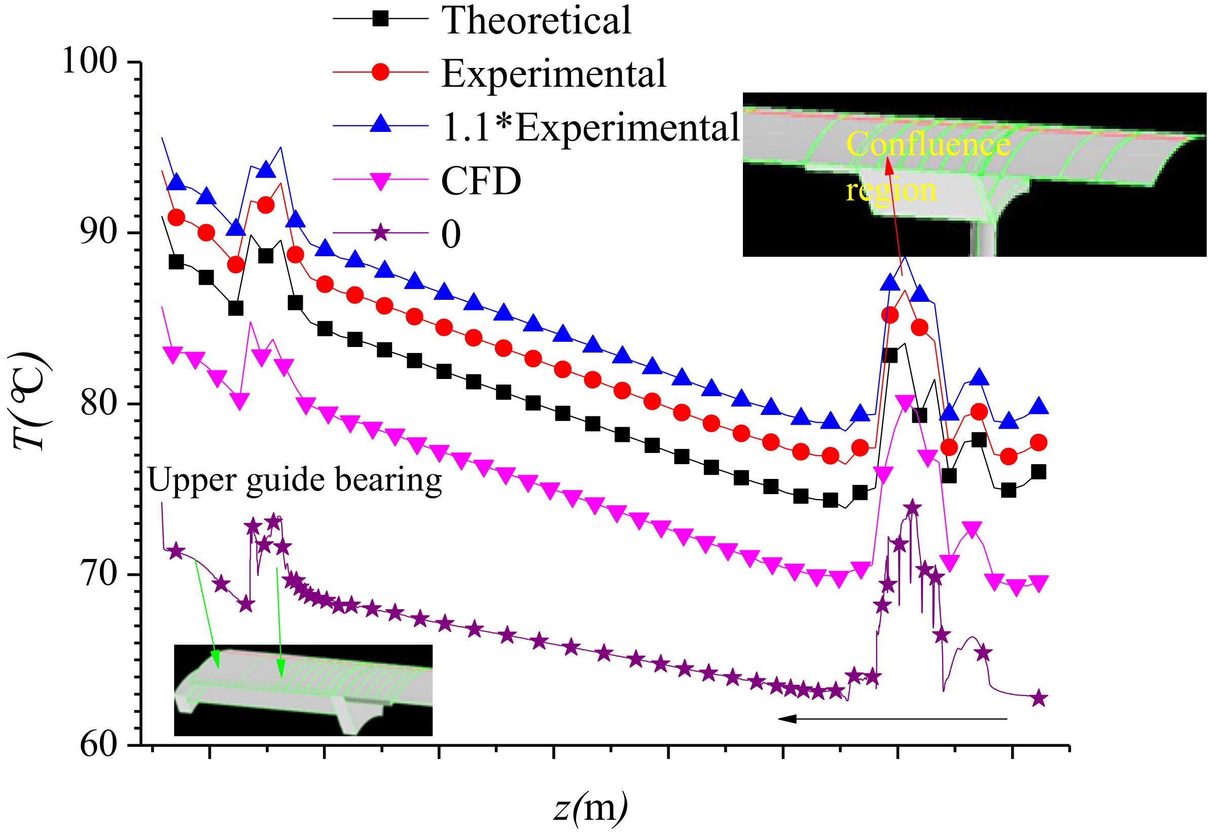
4.2. Temperature Analysis of the Primary Water Passage

Figure 8 shows the temperature distribution of Sampling Line 3 in the internal water passage between the stator and rotor shield. It can be seen from Figure 2 that Sampling Line 3, in turn, through the water clearance at the position of the upper guide bearing, double cans, near the confluence region, and approximately no water flowing area at the bottom of the lower flywheel, increased in the direction of the z-axis. The annular cross-sectional area of water in the confluence region became larger, whereas in the other region, the cross-sectional width was in mm.

It can be seen in Figure 8 that the temperature of water rise was linear between the double cans region, and the cross-sectional area of water was the same. The maximum water temperature value for the four conditions of water friction loss was no more than the alarm temperature of 90 °C; however, the calculation results of the position of the upper guide bearing were inconsistent. The frictional loss did not exceed the temperature when calculated using CFD and the theoretical method, but in the other two cases, local temperature exceeded the rated condition. This example shows that the different calculation methods of friction loss had an influence on the conclusion about whether the water of the upper guide bearing was over temperature or not. It can provide a reference for the design of the internal water passage. The average temperature of water corresponding to the experimental friction loss value of Sampling Line 3 was higher by 2.6 °C than that of the analysis value calculated at the same position, and was lower by about 2.0 °C than the assumed value. For the CFD case, the average value of the temperature of Sampling Line 3 was lower by about 4.8 °C than that of the analysis value calculated at the same position. The average temperature of the water was 8.2 °C higher than that without friction loss.

The sudden rise of the temperature of two local positions is indicated in Figure 8. In the clearance (gap) of the upper guide bearing, the temperature of the water increased linearly, and the temperature of the water near the exit, at the bottom of the upper flywheel, increased dramatically due to the heat source in it. In the water clearance near the confluence region, there was an approximately no water flow region, so a lower rate of heat transfer was in this area. The water temperature was higher than that of the inlet of the rotor shield sleeve.

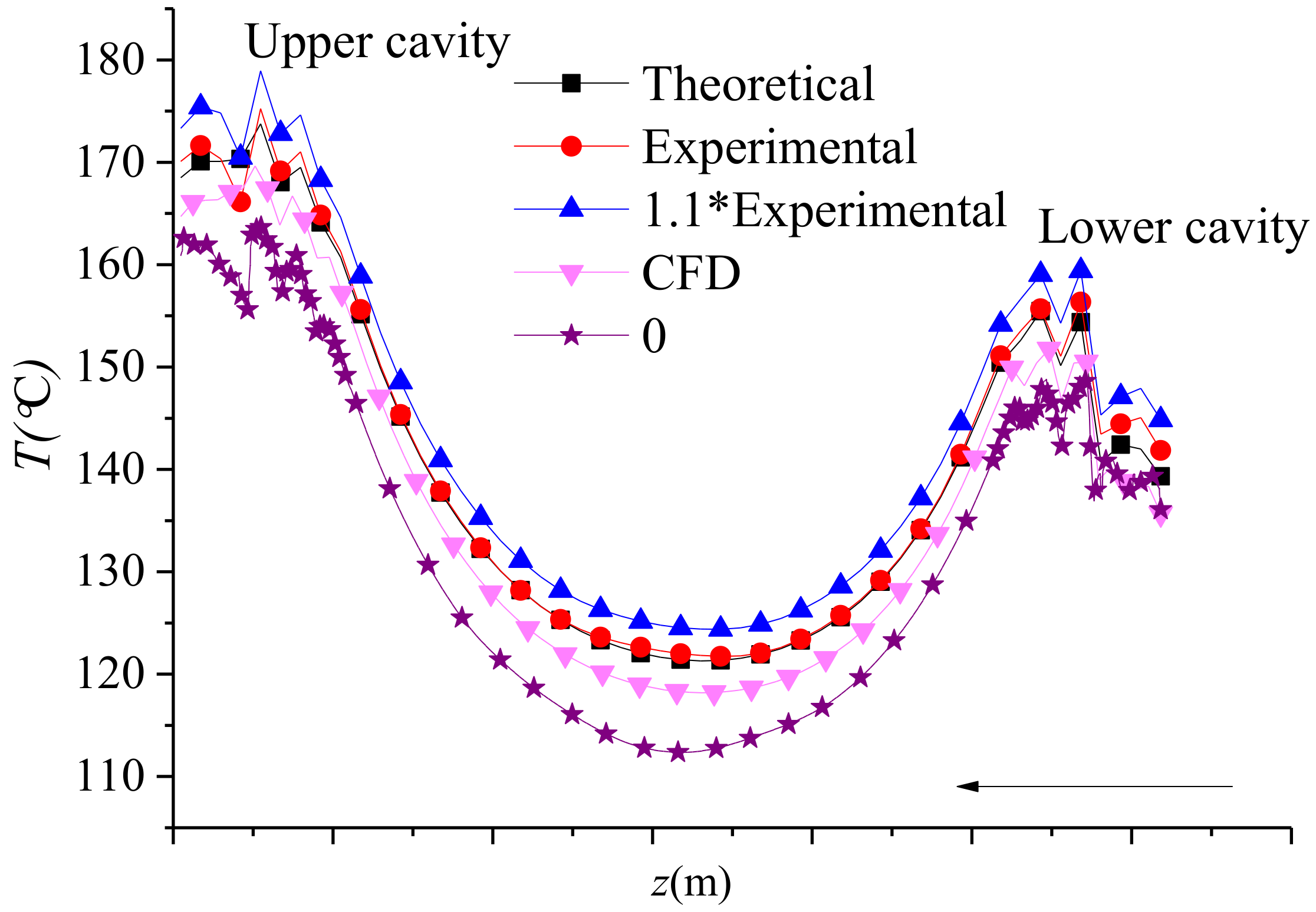
4.3. Temperature Analysis of the Rotor Copper Bar

Figure 9 shows the temperature variations of the sampling line of the rotor copper bar along the z-axis for the five conditions of water friction losses. It shows that the temperature distribution characteristics of the rotor cooper bar were different from the stator winding mentioned above in Figure 6 and Figure 7. The temperature of the rotor copper strip at the lower and upper end loop position rose dramatically, and the temperature gradient was larger because there was a large heat source of electrical loss in the end ring.

The average temperature of the rotor copper bar of Sampling Line 4 corresponding to the analysis of friction loss value was lower by about 1.9 °C and 4.5 °C than that by the experimental value and by assuming 1.1-times the experimental value, respectively, and when friction losses were ignored, it was lower by 14.82 °C than that corresponding to the analysis of the friction loss value. The value of the average temperature of Sampling Line 4 was lower by about 4.71 °C than that of the calculated analysis value, when calculated by the CFD module. It shows that the large friction loss had a relatively large influence on the temperature rise of the rotor bar.

4.4. Temperature Analysis of the Rotor Iron Core

Figure 10 shows the temperature variations of Sampling Line 5 of the rotor iron core tooth along the z-axis for the five conditions of water friction losses, and it can be seen that the temperature distribution characteristics of rotor iron core were similar to Figure 9, different from Figure 6 and Figure 7. There was a sharp rise in the local temperature gradient due to large electric loss in the tooth plate and in the end ring that were located in the lower and upper end of the rotor core, and the temperature distribution of the rotor iron core tooth changed linearly in the double cans section. The temperature of the rotor iron core also gradually increased, and the characteristics were the same as mentioned in the above Figure 9, while only the peak value was different.

It can be concluded that the characteristics of the temperature distribution curves did not change when the calculating method of water friction loss changed (as can be seen in Figure 6, Figure 7, Figure 8, Figure 9 and Figure 10), and the value of the temperature (in Figure 8, Figure 9 and Figure 10) was the highest at the same position under the water friction loss condition of 1.1-times the experimental value and lowest when calculated by the CFD module.

4.5. Accuracy Analysis of Temperature Calculation Results

The temperature calculations obtained at different water friction loss conditions had very small differences from each other. The position of peak temperature corresponding to the analysis value of the loss was same, but the peak value difference was −1.2 °C, when compared with the result of the earlier finite difference method software, which was developed by the factory.

Additionally, under the no load operating condition, multi-point temperature measurement had been performed. To verify the accuracy of the calculation results, the same numerical method (the water friction loss per unit volume was set as heat sources in the corresponding clearance of water) was adopted to calculate the temperature field under the no-load test condition. The error in the temperature results on the many positions simulated (using the method mentioned above) was 5% lower than the test values. However, at present, the thermal test of the motor in the fully-loaded condition has not yet been performed.

The results in this paper were accurate and satisfied the engineering requirements.

5. Conclusions

In this paper, a canned motor has been taken as an example, and a method was presented to study the effect of friction losses on the calculation of the thermal field of the motor using the CFD FLUENT software, that is: the water friction loss per unit volume was added in the corresponding position as the heat source; the viscous heating item option was kept inactive; and the wall roughness in the boundary conditions was not set. For the second method, the friction losses was calculated by the CFD FLUENT software, whereby the option of the viscous heating item was selected, which is right under the turbulence model list, and the wall roughness in the boundary conditions was set according to the different positions of the cans. The conclusion are as follows:

• The peak temperature of the motor winding was lower by −4.2% as compared to the water friction loss calculated by CFD with the proposed water friction loss per unit volume method. This method of, i.e., using given experimental water friction loss per unit volume as the source term did not change the characteristics of the temperature distribution of the components of the motor and intercooling water.
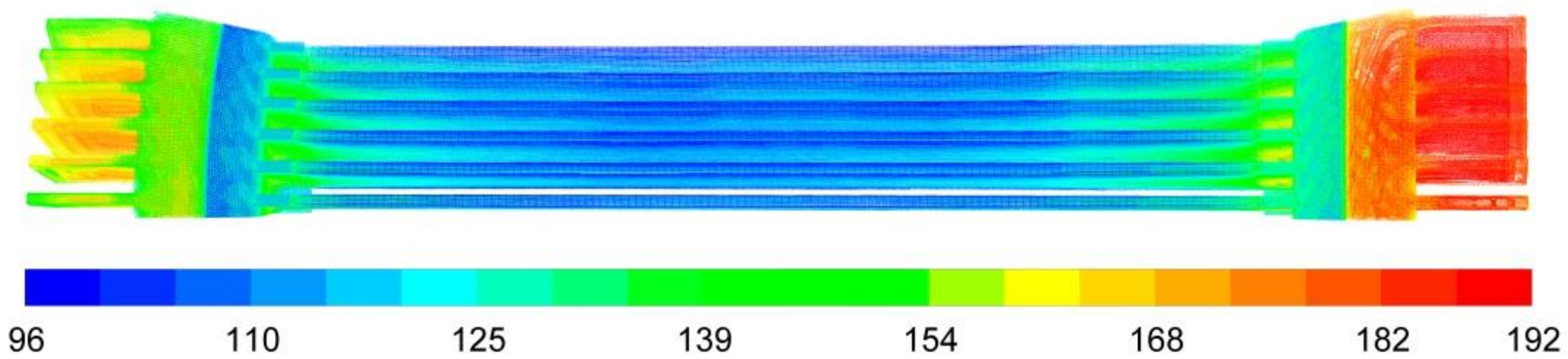
• The temperature along the axial direction increased with the increase of friction loss at the same position of the rotor copper bar, rotor iron core, and for water in the clearance of double cans, and the tendency of the temperature distribution increased linearly along the axial direction where the shield was located.
• The temperature distribution of the winding presented a concave curve, and the lowest temperature point in the upper and lower winding was near the axial center of the winding.
• For the water-cooled shielded motor, the water friction loss cannot be ignored. The calculation method of the water friction loss had a great influence on the conclusion about whether the water of the upper guide bearing was over temperature.

References

- Boglietti, A.; Cavagnino, A. Evolution and modern approaches for thermal analysis of electrical machines. IEEE Trans. Ind. Electron. 2009, 56, 871–882. [Google Scholar] [CrossRef]
- Yetgin, A.G. Effects of induction motor end ring faults on motor performance. Experimental results. Eng. Fail. Anal. 2009, 96, 374–383. [Google Scholar] [CrossRef]
- Liang, Y.; Bian, X.; Yu, H.; Li, C. Finite-element evaluation and eddy-current loss decrease in stator end metallic parts of a large double-canned induction motor. IEEE Trans. Ind. Electron. 2015, 62, 6779–6785. [Google Scholar] [CrossRef]
- Huang, Z.; Fang, J.; Liu, X.; Han, B. Loss calculation and thermal analysis of rotors supported by active magnetic bearings for high-speed permanent-magnet electrical machines. IEEE Trans. Ind. Electron. 2016, 63, 2027–2035. [Google Scholar] [CrossRef]
- Chiu, H.C.; Jang, J.H.; Yan, W.M.; Shiao, R.B. Thermal performance analysis of a 30 kW switched reluctance motor. Int. J. Heat Mass Tran. 2017, 114, 145–154. [Google Scholar] [CrossRef]
- Kim, C.; Lee, K.S. Thermal nexus model for the thermal characteristic analysis of an open-type air-cooled induction motor. Appl. Therm. Eng. 2017, 112, 1108–1116. [Google Scholar] [CrossRef]
- Kim, C.; Lee, K.S. Numerical investigation of the air-gap flow heating phenomena in large-capacity induction motors. Int. J. Heat Mass Tran. 2017, 110, 746–752. [Google Scholar] [CrossRef]
- Lu, Y.; Liu, L.; Zhang, D. Simulation and analysis of thermal fields of rotor multislots for nonsalient-pole motor. IEEE Trans. Ind. Electron. 2015, 62, 7678–7686. [Google Scholar] [CrossRef]
- Lancial, N.; Torriano, F.; Beaubert, F.; Harmand, S.; Rolland, G. Study of a Taylor-Couette-Poiseuille flow in an annular channel with a slotted rotor. In Proceedings of the International Conference on Electrical Machines (ICEM), Hangzhou, China, 2–5 September 2014; pp. 1422–1429. [Google Scholar]
- Traxler-Samek, G.; Zickermann, R.; Schwery, A. Cooling airflow, losses, and temperatures in large air-cooled synchronous machines. IEEE Trans. Ind. Electron. 2010, 57, 172–180. [Google Scholar] [CrossRef]
- Tu, J.; Yeoh, G.H.; Liu, C. Computational Fluid Dynamics: A Practical Approach, 3rd ed.; Butterworth-Heinemann: Oxford, UK, 2018. [Google Scholar]
- Luomi, J.; Zwyssig, C.; Looser, A.; Kolar, J.W. Efficiency optimization of a 100-W 500,000-r/min permanent-magnet machine including air-friction losses. IEEE Trans. Ind. Appl. 2009, 45, 1368–1377. [Google Scholar] [CrossRef]
- Gengji, W.; Ping, W. Rotor loss analysis of PMSM in flywheel energy storage system as uninterruptable power supply. IEEE Trans. Appl. Superconduct. 2016, 26, 1–5. [Google Scholar] [CrossRef]
- Aglen, O.; Andersson, A. Thermal analysis of a high-speed generator. In Proceedings of the 38th IAS Annual Meeting on Conference Record of the Industry Applications Conference, Salt Lake City, UT, USA, 12–16 October 2003; Volume 1, pp. 547–554. [Google Scholar]
- Le, Y.; Sun, J.; Han, B. Modeling and design of 3-DOF magnetic bearing for high-speed motor including eddy-current effects and leakage effects. IEEE Trans. Ind. Electron. 2016, 63, 3656–3665. [Google Scholar] [CrossRef]
- Zhang, F.; Du, G.; Wang, T.; Wang, F.; Cao, W.; Kirtley, J.L. Electromagnetic design and loss calculations of a 1.12-MW high-speed permanent-magnet motor for compressor applications. IEEE Trans. Energy Convers. 2016, 31, 132–140. [Google Scholar] [CrossRef]
- Lomax, H.; Pulliam, T.H.; Zingg, D.W. Fundamentals of Computational Fluid Dynamics, 1st ed.; Springer Science & Business Media: Berlin, Germany, 2013. [Google Scholar]
- Heins, G.; Ionel, D.M.; Patterson, D.; Stretz, S.; Thiele, M. Combined experimental and numerical method for loss separation in permanent-magnet brushless machines. IEEE Trans. Ind. Appl. 2016, 52, 1405–1412. [Google Scholar] [CrossRef]
- Saari, J. Thermal Analysis of High-Speed Induction Machines. Ph.D. Dissertation, Department of Electrical and Communications Engineering, Helsinki University of Technology, Espoo, Finland, 1998. [Google Scholar]