Economic MPC of Wastewater Treatment Plants Based on Model Reduction

Abstract

In this paper, we consider the problem of economic model predictive control of wastewater treatment plants based on model reduction. We apply two model approximation methods to a wastewater treatment plant (WWTP) described by a modified Benchmark Simulation Model No.1 to overcome the intensive computation associated with economic model predictive control (MPC). Two computationally efficient models are obtained based on trajectory piecewise linearization (TPWL) and reduced order TPWL. To obtain the reduced order TPWL model, a proper orthogonal decomposition (POD)-based method is utilized. Further, the reduced order model is linearized to obtain a TPWL-POD model. The objective is to design controllers which minimize the overall economic cost. Accordingly, we design economic MPC (EMPC) controllers based on each of the models. The economic control cost can be described as a weighted summation of effluent quality and overall operating cost. We compare the accuracy of the two proposed approximation models with different linearization point numbers. We evaluate the average evaluation time for the two proposed EMPC controllers and make comparisons with the EMPC based on the original nonlinear model. We also investigate how the number of linearization points involved in the TPWL model and TPWL-POD model affects the control performance in terms of average performance cost and the average evaluation time.

1. Introduction

Wastewater treatment plants (WWTPs) have been widely used to recycle wastewater in order to minimize its adverse environmental impacts. A typical WWTP is a large-scale nonlinear process that consists of a series of interconnected biological reactors and a secondary settler. While meeting the strict requirements in environmental regulations, ensuring the process safety and minimizing the cost of operation, a wastewater treatment plant should be monitored and regulated [1]. However, significant variability of inlet flow rates and wastewater compositions leads to the increased complexity in the design of advanced control and monitoring schemes for WWTPs [2].

In the literature, there are many existing resutls on the control of WWTPs. For example, in [3], proportional-integral (PI) was used to control a nutrient removal WWTP. In [4], the tuning of proportional-integral-derivative control was considered in the control of the dissolved oxygen concentration in the activated sludge process. Advanced control methods such as model predictive control (MPC) have also attracted much research attention in the control of WWTPs. In [5,6,7], simultaneous design and control of WWTPs were considered with MPC. In [8], an MPC controller was developed for the Benchmark Simulation Model No.1 (BSM1). MPC was also used to in the control of oxygen concentration in [9,10]. In [11,12], MPC was applied to a WWTP to increase the plant efficiency, and in [13] it was applied to reduce the power usage. In one of our previous works, we applied economic MPC (EMPC) to explicitly optimize the operating economics of WWTPs [14]. While the EMPC can lead to improved effluent quality and improved overall operating cost, its high evaluation time renders the online implementation of this economic MPC intractable.

When considering economic MPC, it in general requires more time to evaluate the corresponding optimization problem compared with the traditional tracking MPC. One way to address the high evaluation time of economic MPC of nonlinear system is to use a distributed computing framework. Following this idea, in a recent work [1], we developed distributed EMPC schemes for WWTPs to reduce the evaluation time of the centralized EMPC. In this work, we consider another approach to address the high evaluation time of economic MPC; that is, to design economic MPC based on approximated models. This is based on the consideration that when solving the nonlinear optimization problem of an economic MPC, the model of the system is evaluated many times. If we can use an approximated model that can be evaluated faster, then the economic MPC can be evaluated faster.

The objective of this work is to study how two model approximation methods can help speed up the evaluation of the optimization problem of economic MPC. Specifically, we propose to develop linear approximated models of the original nonlinear system and use the approximated models in EMPC design. A lot of achievements have been made on the use of approximated models in MPC. The work of [15] applied feedback linearization to the plant and then used MPC in a cascade arrangement for the resulting linear system. The nonlinear programming problem was reduced to a quadratic optimization problem which can improve the computational efficiency. The implementation of MPC with a different linear model at each time step derived from a local (Jacobian) linearization of the nonlinear plant was first proposed in [16]. An extended Kalman filter was proposed to be added to this approach to deal with unstable nonlinear process and ensure a better disturbance rejection in [17,18]. This idea was further developed in [19], contraction constraints were applied and the explicit stability conditions were derived. In [20], one technique was proposed to approximate the nonlinear system with a linear time varying (LTV) model, which is obtained from a linearization of the system along the predicted system trajectory. In [21,22], a novel MPC algorithm was proposed which can significantly reduce the online evaluation time. The approach is to only compute the first control move while approximating the rest of control moves by using a linear controller.

Pertaining to model approximation, model order reduction techniques are also popular and can significantly abate the complexity of the nonlinear system while conserving the dominant dynamics of the process [23]. The proper orthogonal decomposition (POD) method is extensively used in data analysis for approximating the high-dimensional process by low-dimensional descriptions [24]. The POD method has been widely applied in control in chemical engineering [25,26,27,28,29]. In [30], a state estimation scheme was established for WWTPs using POD-based model approximation. In [31,32], a reduced order model based on the POD-Galerkin projection method was constructed for economic MPC. With the reduced order model, the evaluation time of the economic MPC was significantly reduced. In [33], a nonlinear system was represented by a piecewise-linear system and each of the pieces were reduced with a Krylov projections.

In this work, we apply the trajectory piecewise linearization and a combination of trajectory piecewise linearization and proper orthogonal decomposition method to WWTPs to derive low-order linear models, which are subsequently used for EMPC controller design. The model accuracy, economic MPC evaluation time, and economic control performance of the WWTP process under these EMPC controllers are compared. Note that we investigate the performance of these model approximation and reduction methods in a centralized control framework. These methods may also be used together with distributed control to further reduce the evaluation time of the centralized EMPC. The main contributions of this work include the folllowing:

• The investigation of two model approximation methods in EMPC evaluation time reduction in the context of wastewater treatment control.
• The detailed model reduction procedures for wastewater treatment processes and the design of EMPC based on the reduced models.
• Extensive simulation results and analysis on the performance of EMPC based on reduced models in terms of economic performance and controller evaluation time.

2. Preliminaries

2.1. WWTP Process Description and Modeling

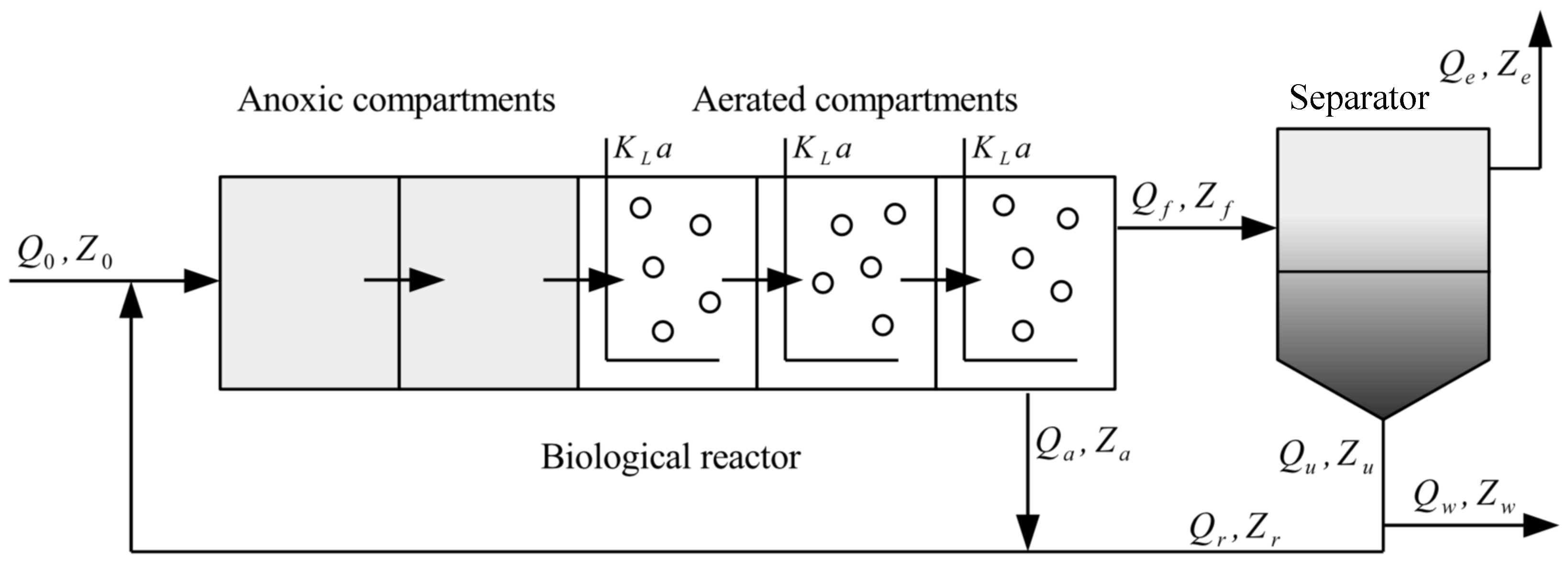
The WWTP process considered in this work is a modified version of the Benchmark Simulation Model No.1 (BSM1). A schematic of the process is shown in Figure 1. The process consists of a sludge reactor consisting of five compartments and an ideal separator [34]. In the sludge reactor, the first two compartments are anoxic compartments and the remaining three compartments are aerobic compartments. During the operation, denitrification reactions occur in the anoxic compartments where nitrate is converted to nitrogen, while nitrification reactions take place in three aerobic compartments where ammonium is oxidized to nitrate. In the process, the inlet stream of the first compartment of the reactor includes a feed stream, an internal recycle stream and an external recycle stream. The wastewater enters the first compartment of the reactor in the feed stream at flow rate $Q_0$ and concentration $Z_0$. The internal recycle stream is a portion of the effluent from the last aerated compartment of the reactor at flow rate $Q_a$ and concentration $Z_a$. The other portion of the effluent enters the ideal separator at flow rate $Q_f$ and concentration $Z_f$. The external recycle stream is a portion of the underflow of the separator and it is fed back into the first compartment of the reactor at flow rate $Q_r$ and concentration $Z_r$. The remaining portion of the underflow which is the generated sludge leaves the separator at flow rate $Q_w$ and concentration $Z_w$. The purified water leaves the process via the overflow of the separator at flow rate $Q_e$ and concentration $Z_e$. According to [35], eight basic biological reactions are taken into account, and the concentrations of 13 major reaction-involved compounds defined in

Table 1. Definition and notation of the process variables in the modified BSM1 model.

Definition	Notation	Unit
inert soluble organic matter	$S_I$	$\mathrm{g}\mathrm{COD}·{\mathrm{m}}^{-3}$
inert particulate organic matter	$X_I$	$\mathrm{g}\mathrm{COD}·{\mathrm{m}}^{-3}$
readily biodegradable and soluble substrate	$S_s$	$\mathrm{g}\mathrm{COD}·{\mathrm{m}}^{-3}$
slowly biodegradable and soluble substrate	$X_s$	$\mathrm{g}\mathrm{COD}·{\mathrm{m}}^{-3}$
biomass of active autotrophs	$X_{B_A}$	$\mathrm{g}\mathrm{COD}·{\mathrm{m}}^{-3}$
biomass of active heterotrophs	$X_{B_H}$	$\mathrm{g}\mathrm{COD}·{\mathrm{m}}^{-3}$
particulate generated from decay of organisms	$X_P$	$\mathrm{g}\mathrm{COD}·{\mathrm{m}}^{-3}$
particulate biodegradable organic nitrogen	$X_{ND}$	$\mathrm{g}\mathrm{N}·{\mathrm{m}}^{-3}$
nitrite nitrogen and nitrate	$S_{NO}$	$\mathrm{g}\mathrm{N}·{\mathrm{m}}^{-3}$
free and saline ammonia	$S_{NH}$	$\mathrm{g}\mathrm{N}·{\mathrm{m}}^{-3}$
biodegradable and soluble organic nitrogen	$S_{ND}$	$\mathrm{g}\mathrm{N}·{\mathrm{m}}^{-3}$
dissolved oxygen	$S_O$	$\mathrm{g}(-\mathrm{COD})·{\mathrm{m}}^{-3}$
alkalinity	$S_{ALK}$	$\mathrm{mol}·{\mathrm{m}}^{-3}$
total sludge concentration in settler	X	$\mathrm{g}\mathrm{COD}·{\mathrm{m}}^{-3}$

are the state variables of this model.

The dynamics of WWTP based on the modified BSM1 model can be described by 78 ordinary differential equations. The dynamics of each compartment of the reactor and the ideal separator can be described by 13 differential equations according to 13 state variables defined in Table 1. The parameter values of this process model are reported in [2] and

Table 2. Parameter value of the modified BSM1 model.

$V_1$ (volume of compartment 1)	1000 ${\mathrm{m}}^3$
$V_2$ (volume of compartment 2)	1000 ${\mathrm{m}}^3$
$V_3$ (volume of compartment 3)	1333 ${\mathrm{m}}^3$
$V_4$ (volume of compartment 4)	1333 ${\mathrm{m}}^3$
$V_5$ (volume of compartment 5)	1333 ${\mathrm{m}}^3$
$Q_w$ (Underflow discharge flow rate)	385 ${\mathrm{m}}^3·{\mathrm{d}}^{-1}$
$Q_r$ (Outer recycle flow rate)	$18,446$${\mathrm{m}}^3·{\mathrm{d}}^{-1}$
$V_s$ (Volume of separator)	6000 ${\mathrm{m}}^3$
$K_L{a}_3$ (Oxygen transfer coefficient of chamber 3)	240 ${\mathrm{d}}^{-1}$
$K_L{a}_4$ (Oxygen transfer coefficient of chamber 4)	240 ${\mathrm{d}}^{-1}$

shows the model parameters adopted in this work. The dynamics of the system are described based on mass balance as follows:

For compartment k ($k=1$) of the biological reactor:

$$\begin{array}{cc}\hfill \frac{d{Z}_1}{dt}& =\frac{1}{V_1}(Q_a{Z}_a+Q_r{Z}_r+Q_0{Z}_0+r_1{V}_1-Q_1{Z}_1)\hfill \end{array}$$

(1)

$$\begin{array}{cc}\hfill Q_1& =Q_a+Q_r+Q_0\hfill \end{array}$$

(2)

For compartment k ($k=2,\cdots ,5$) of the biological reactor:

$$\begin{array}{cc}\hfill \frac{d{Z}_k}{dt}& =\frac{1}{V_k}(Q_{k-1}{Z}_{k-1}+r_k{V}_k-Q_k{Z}_k)\hfill \end{array}$$

(3)

$$\begin{array}{cc}\hfill Q_k& =Q_{k-1}\hfill \end{array}$$

(4)

Special case for concentration $S_{O,k}$, $k=1,\cdots ,5$, (the concentration of dissolved oxygen in compartment k of the biological reactor):

$$\begin{array}{cc}\hfill \frac{d{S}_{O,k}}{dt}& =\frac{1}{V_k}(Q_{k-1}{S}_{O,k-1}+r_k{V}_k+K_L{a}_k{V}_k(S_O^{\ast }-S_{O,k})-Q_k{S}_{O,k})\hfill \end{array}$$

(5)

In Equations (1), (3) and (5), $Z_k$ is the concentration of the compounds defined in Table 1 in kth compartment of the biological reactor, $V_k$ represents the volume of kth compartment, $r_k$ denotes the observed conversion rates of the compound in kth compartment, $S_O^{\ast }$ is the saturation concentration for oxygen and is equal to $8\mathrm{g}·{\mathrm{m}}^{-3}$, and $K_L{a}_k$ represents the oxygen transfer coefficient in kth compartment, since compartment 1 and 2 of the reactor are anoxic compartments, $K_L{a}_1=K_L{a}_2=0{\mathrm{d}}^{-1}$ [2].

The ideal separator is assumed to be a membrane filtration unit and no biological activity exists in it [34]. All soluble compounds (i.e., $S_I$, $S_S$, $S_O$, $S_{NO}$, $S_{NH}$, $S_{ND}$, and $S_{ALK}$) are assumed to be well-mixed in the separator, and all solid compounds (i.e., $X_I$, $X_S$, $X_{B,H}$, $X_{B,A}$, $X_P$, and $X_{ND}$) are assumed to precipitate in the bottom of the separator [36]. Based on mass balance, the dynamics of the separator unit ($k=6$) can be described as follows:

For soluble compounds in the separator unit ($k=6$):

$$\begin{array}{cc}\hfill \frac{d{Z}_k}{dt}& =\frac{1}{V_k}(Q_f{Z}_f+Q_e{Z}_e+Q_r{Z}_r+Q_w{Z}_w)\hfill \end{array}$$

(6)

$$\begin{array}{cc}\hfill Z_e& =Z_r=Z_w=Z_k\hfill \end{array}$$

(7)

$$\begin{array}{cc}\hfill Z_f& =Z_{k-1}=Z_k\hfill \end{array}$$

(8)

For solid compounds in the separator unit ($k=6$):

$$\begin{array}{cc}\hfill \frac{d{Z}_k}{dt}& =\frac{1}{V_k}(Qf{Z}_f+Q_r{Z}_r+Q_w{Z}_w)\hfill \end{array}$$

(9)

$$\begin{array}{cc}\hfill Z_r& =Z_w=Z_k\hfill \end{array}$$

(10)

$$\begin{array}{cc}\hfill Z_f& =Z_{k-1}=Z_k\hfill \end{array}$$

(11)

The flow rates of each stream in Figure 1 can be described as follows:

$$\begin{array}{cc}\hfill Q_1& =Q_2=Q_3=Q_4=Q_5\hfill \end{array}$$

(12)

$$\begin{array}{cc}\hfill Q_1& =Q_a+Q_r+Q_0\hfill \end{array}$$

(13)

$$\begin{array}{cc}\hfill Q_f& =Q_5-Q_a=Q_e+Q_r+Q_w=Q_e+Q_u\hfill \end{array}$$

(14)

$$\begin{array}{cc}\hfill Q_0& =Q_e+Q_w\hfill \end{array}$$

(15)

2.2. Compact form of the System Model

The modified BSM1 model for the wastewater treatment plant can be described in the following compact form:

$$\dot{x}\left(t\right)=f(x\left(t\right),u\left(t\right))$$

(16)

where $x\in {\mathbb{R}}^{78}$ is the vector of process states, $u\in {\mathbb{R}}^3$ represents the input vector consisting manipulated inputs and the uncontrolled inputs. The manipulated inputs are the flow rate of the recirculation stream (i.e., $Q_a$) and the oxygen transfer rate in the fifth compartment of the biological reactor (i.e., $K_L{a}_5$), respectively. The uncontrolled inputs contain the influent information under different weather conditions.

2.3. Economic Control Objective

The economic control objective is defined as follows:

$$\begin{array}{cc}\hfill l_{eco}(x\left(\tau \right),u\left(\tau \right))& ={\alpha }_{EQ}\widehat{EQ}\left(\tau \right)+{\alpha }_{OCI}\widehat{OCI}\left(\tau \right)\hfill \end{array}$$

(17)

where $\widehat{EQ}$ is the economic index of effluent quality (EQ) which is calculated as the average amount of the pollutants discharged and is defined in Equation (18), $\widehat{OCI}$ represents the average amount of the overall cost index (OCI) which contains the factors that affect the operating costs significantly and it is defined in Equation (23), ${\alpha }_{EQ}$ and ${\alpha }_{OCI}$ are two weighting coefficients for EQ and OCI, respectively.

2.3.1. Effluent Quality

In BSM1, EQ ($\mathrm{kg}\mathrm{pollution}\mathrm{unit}·{\mathrm{day}}^{-1}$) represents the daily average of a weighted summation of the effluent concentrations of several compounds, which significantly affect the quality of the processed water according to regional regulations. Specifically, the EQ index is evaluated as follows:

$$\begin{array}{c}\hfill \mathrm{EQ}=\frac{1}{T·1000}{\int }_{t_0}^{t_f}\left(\begin{array}{cc}\hfill {\beta }_{\mathrm{SS}}& ·{\mathrm{SS}}_e\left(t\right)+{\beta }_{\mathrm{COD}}·{\mathrm{COD}}_e\left(t\right)+{\beta }_{NKj}·S_{NKj,e}\left(t\right)\hfill \\ \hfill & +{\beta }_{NO}·S_{NO,e}\left(t\right)+{\beta }_{\mathrm{BOD}}·{\mathrm{BOD}}_e\left(t\right)\hfill \end{array}\right)Q_e\left(t\right)dt\end{array}$$

(18)

where

$$\begin{array}{cc}\hfill {\mathrm{SS}}_e=& 0.75\left(X_{S,e}+X_{B_A,e}+X_{B_H,e}+X_{I,e}+X_{P,e}\right)\hfill \\ \hfill {\mathrm{COD}}_e=& S_{I,e}+S_{S,e}+X_{S,e}+X_{I,e}+X_{B_H,e}+X_{B_A,e}+X_{P,e}\hfill \\ \hfill {\mathrm{BDO}}_e=& 0.25\left(S_{S,e}+X_{S,e}+\left(1-f_p\right)\left(X_{B_A,e}+X_{B_H,e}\right)\right)\hfill \\ \hfill S_{NKj,e}=& S_{ND,e}+S_{NH,e}+X_{ND,e}+i_{XB}\left(X_{B_A,e}+X_{B_H,e}\right)+i_{XP}\left(X_{I,e}+X_{P,e}\right)\hfill \end{array}$$

In Equation (18), $t_0$ and $t_f$ denote the initial and final time instants of the evaluation horizon; $T:=t_f-t_0$ is the length of the horizon, and is usually selected to be $T=7\mathrm{days}$; SS represents the concentration of suspended solids, COD is chemical oxygen demand, BOD denotes the biological oxygen demand, and $S_{\mathrm{NKj}}$ denotes the concentration of Kjeldahl nitrogen; ${\beta }_{\mathrm{SS}}$, ${\beta }_{\mathrm{COD}}$, ${\beta }_{NKj}$, ${\beta }_{NO}$ and ${\beta }_{\mathrm{BOD}}$ represent the weighting coefficients used to calculate EQ; $f_p$, $i_{XB}$, and $i_{XP}$ are stoichiometirc parameters. The corresponding values are listed in

Table 3. Values of the weighting coefficients of EQ Index.

Weighting Coefficient	${\mathit{\beta }}_{\mathbf{SS}}$	${\mathit{\beta }}_{\mathbf{COD}}$	${\mathit{\beta }}_{\mathit{N}\mathit{K}\mathit{j}}$	${\mathit{\beta }}_{\mathit{N}\mathit{O}}$	${\mathit{\beta }}_{\mathbf{BOD}}$	${\mathit{f}}_{\mathit{p}}$	${\mathit{i}}_{\mathit{X}\mathit{B}}$	${\mathit{i}}_{\mathit{X}\mathit{P}}$
Value	2	1	30	10	2	0.08	0.08	0.06

[37] and the subscript “e” refers to the effluent of the secondary settler.

2.3.2. Overall Cost Index

The total operating cost required for processing wastewater is another important factor in performance evaluation. Factors that have major effects on the operating cost include the sludge production that needs to be disposed, the energy required for aerating and pumping, external carbon consumption as well as mixing energy.

The sludge production (SP) is defined as the average amount per day ($\mathrm{kg}·{\mathrm{day}}^{-1}$) of the solids produced in the process over the evaluation horizon T, including the solids discharged through the wastage flow $Q_w$ from the settler and the sedimentary solids in a WWTP plant.

$$\begin{array}{cc}\hfill \mathrm{SP}=& \frac{0.75}{T·1000}{\int }_{t_0}^{t_f}\left(X_{S,w}\left(t\right)+X_{I,w}\left(t\right)+X_{B_A,w}\left(t\right)+X_{B_H,w}\left(t\right)+X_{P,w}\left(t\right)\right)Q_w\left(t\right)dt\hfill \\ \hfill & +\frac{1}{T·1000}(\mathrm{SS}\left(t_f\right)-\mathrm{SS}\left(t_0\right))\hfill \end{array}$$

(19)

In Equation (19), the subscript “w” refers to the wastage outlet of the secondary settler.

The aeration energy (AE) ($\mathrm{kWh}·{\mathrm{day}}^{-1}$) is associated with several plant characteristics, including the diffuser type, the submersion depth, the bubble size, etc. AE is calculated based on the oxygen transfer rates (i.e., $K_L{a}_i$, $i=1,\dots ,5$) by considering an immersion depth of 4 m as follows:

$$\begin{array}{c}\hfill \mathrm{AE}=\frac{S_o^{sat}}{T·1800}{\int }_{t_0}^{t_f}\sum _{i=1}^5{V}_i·K_L{a}_i\left(t\right)dt\end{array}$$

(20)

where $i\in \left\{12345\right\}$, $V_i$ denotes the volume of the i-th chamber of the sludge reactor, and $K_L{a}_i$ denotes the oxygen transfer rate in the i-th chamber. $S_o^{sat}$ denotes the saturation concentration of oxygen and its value is 8 $\mathrm{g}/{\mathrm{m}}^3$.

The pumping energy (PE) ($\mathrm{kWh}·{\mathrm{day}}^{-1}$) represents the energy consumed by the pumps used for inner recycle (i.e., $Q_a$) and outer recycle (i.e., $Q_r$). PE is calculated as below:

$$\begin{array}{c}\hfill \mathrm{PE}=\frac{1}{T}{\int }_{t_0}^{t_f}\left(0.004Q_a\left(t\right)+0.05Q_w\left(t\right)+0,008Q_r\left(t\right)\right)dt\end{array}$$

(21)

The mixing energy (ME) ($\mathrm{kWh}·{\mathrm{day}}^{-1}$) denotes the energy consumed for mixing the compounds in the anoxic chambers to avoid the occurrence of settling. ME is calculated depending on the volume of each chamber and the oxygen transfer rates:

$${\displaystyle \mathrm{ME}=\frac{24}{T}{\int }_{t_0}^{t_f}\left({\displaystyle \sum _{i\in \mathbb{I}}0.005·V_i}\right)dt}$$

(22)

where $\mathbb{I}:=\left\{i|i\in \left\{12345\right\}\right\}$.

The overall cost index (OCI) approximates the total cost for WWTP operation by taking a weighted summation of the listed major factors as follows:

$$\mathrm{OCI}=5·\mathrm{SP}+\mathrm{AE}+\mathrm{PE}+\mathrm{ME}$$

(23)

3. Trajectory Piecewise Linear (TPWL) Model

In this section, the trajectory piecewise linear model approach is introduced and the trajectory piecewise linear model is presented. The steps to generate the piecewise linear model are also shown in this section.

3.1. Piecewise Linear Representation

A linearized model for the nonlinear system can be obtained at a steady-state point ($x_s,u_s$) as follows:

$$\begin{array}{cc}\hfill \frac{dx}{dt}& =f(x_s,u_s)+A(x-x_s)+B(u-u_s)\hfill \end{array}$$

(24a)

$$\begin{array}{cc}\hfill A& =\frac{\partial f}{\partial x}{|}_{x_s,u_s}\hfill \end{array}$$

(24b)

$$\begin{array}{cc}\hfill B& =\frac{\partial f}{\partial u}{|}_{x_s,u_s}\hfill \end{array}$$

(24c)

where A is the Jacobian matrix of system $f(x,u)$ evaluated at the steady-state.

The simple linearized model can be used to approximate weakly nonlinear systems with less evaluation time [33]. The approximated result of the linearized model usually depends on the range of inputs. If the system is a highly nonlinear system, the simple linearized model which is only linearized at one point would be less accurate. The main idea of the piecewise linear model approach is to generate a weighted combination of linear models which are linearized at appropriately selected states of the original nonlinear system. Compared with the system which is linearized at one single point, the system consisting of a combination of multiple linearizations would generate a better approximation result for a more complex nonlinear system.

Assuming that s linearized models have been generated for the nonlinear system of Equation (16) at points $(x_i,u_i)$, $i=0,1,\cdots ,(s-1)$:

$$\begin{array}{cc}\hfill \frac{dx}{dt}& =f(x_i,u_i)+A_i(x-x_i)+B_i(u-u_i)\hfill \end{array}$$

(25a)

$$\begin{array}{cc}\hfill A_i& =\frac{\partial f}{\partial x}{|}_{x_i,u_i}\hfill \end{array}$$

(25b)

$$\begin{array}{cc}\hfill B_i& =\frac{\partial f}{\partial u}{|}_{x_i,u_i}\hfill \end{array}$$

(25c)

A weighted combination of the linearized models in the form of Equation (25) of the nonlinear system leads to the following representation:

$$\begin{array}{cc}\hfill \frac{dx}{dt}& =\sum _{i=0}^{s-1}{w}_i\left(x\right)(f(x_i,u_i)+A_i(x-x_i)+B_i(u-u_i))\hfill \end{array}$$

(26)

where the weight $w_i\left(x\right)$ is a state dependent variable and it can be computed from the distance between current state x and the linearized point $x_i$ [33].

3.2. Generation of Piecewise Linear Model

The trajectory piecewise linear model is developed based on a fixed trajectory of the entire nonlinear system. The fixed trajectory is generated by simulating the nonlinear system based on a fixed training input u. Let us consider that we have generated a fixed trajectory of the nonlinear system, and the initial state $x_0$ is given. The selection of linearization points can be shown as in Algorithm 1.

Algorithm 1: Algorithm for finding the linearization points of piecewise linear model

Define $S=\{0,1,\dots ,N\}$ and $S_p=\left\{\right\}$. Set $i=0$ and $S_l=\left\{x_i\right\}$. If$S\ne S_p$, then: 3.1. Set $x_i$ as one of the linearization points. 3.2. For each $j\in S\backslash S_p$, 3.2.1 Calculate the distance between point $x_j$ and the linearization point $x_i$, $d_j={\parallel x_j-x_i\parallel }_2$. 3.2.2 If$d_j\le \delta$ ($\delta >0$), then:   $S_p=S_p\cup \left\{j\right\}$. Else, do:   $S_p=S_p$. 3.3. Select $k_{min}$ such that $k_{min}=arg\underset{k}{min}\left\{d_k|k\in S\backslash S_p\right\}$. 3.4. Set $i=k_{min}$, set $S_l=S_l\cup \left\{x_i\right\}$. Go to Step 3.1.   Else, end.

In Algorithm 1, the operator “\” denotes set subtraction such that $A\backslash B:=\left\{x\right|x\in A,x\notin B\}$. N is the number of sampled points on this fixed trajectory. $S_l$ is the set of the linearization points. The $\delta$ value is a pre-determined distance threshold, and it can be determined in Algorithm 2. In Algorithm 2, s is the number of models supposed to be generated.

Algorithm 2: Determination of the pre-determined distance threshold $\delta$ value algorithm

Find the maximum distance between any of the two points on the trajectory, $d_j={\parallel x_j-x_h\parallel }_2$, $j,h\in \{0,1,\cdots ,N\}$. Set $\delta =d_{max}/s$.

The state dependent weight $w_i\left(x\right)$ shown in Equation (26) can be computed as described in Algrithm 3 [33].

Algorithm 3: Computation algorithm for the state dependent weight parameter $w_i\left(x\right)$

At each linearization point $(x_i,u_i)$, compute the distance $d_i={\parallel x-x_i\parallel }_2$. Find the minimum value among $d_i$, $m={\min }_{i=0,\cdots ,(s-1)}{d}_i$. For $i=0,\cdots ,(s-1)$ compute ${\widehat{w}}_i=e^{-\beta d_i/m}$. Compute the summation of ${\widehat{w}}_i$, $S\left(x\right)={\sum }_{j=0}^{s-1}{\widehat{w}}_i\left(x\right)$. Compute the normalized parameter $w_i\left(x\right)=\frac{{\widehat{w}}_i\left(x\right)}{S\left(x\right)}$.

In Algorithm 3, $\beta$ is a positive constant value. The weighting parameter $w_i\left(x\right)$ changes according to the position of current state x in state space. The exponential term in step 3 to determine the weighting parameter ensures that the distribution of the weight $w_i$ will change immediately close to one if current state x is sufficiently close to the linearization point $x_i$.

4. TPWL Model Based on POD Method

In this section, the TPWL method is combined with the POD method to further reduce the evaluation time. The POD method is introduced in this section. The steps of establishing the TPWL-POD model are presented and the representation of the model is also shown in this section.

4.1. POD Method Introduction

The POD method can be used to obtain a low-order model but capture the most important dynamics of the original complicated systems [24]. POD method is a SVD-based approximation method to derive the low dimensional system to approximate the large scale system. It can be applied to both high-complexity linear and nonlinear systems [38].

Giving a fixed input u, the trajectory of state $x\in {\mathbb{R}}^n$ at certain time instances $t_k$ can be measured as:

$$\begin{array}{c}\hfill X=\left[x\left(t_1\right)x\left(t_2\right)x\left(t_3\right)\cdots x\left(t_N\right)\right]\end{array}$$

(27)

$X\in {\mathbb{R}}^{n\times N}$ in (27) can be called as the snapshot matrix of the process data. It should be mentioned that the measured time instant points N should be much greater than the dimension of the system n, i.e., $N\gg n$. By computing the singular value decomposition of the snapshot matrix, X can be decomposed into a product of three matrices [38]:

$$\begin{array}{c}\hfill X=U\Sigma V^T\in {\mathbb{R}}^{n\times N}\end{array}$$

(28)

where $U\in {\mathbb{R}}^{n\times n}$ and $V\in {\mathbb{R}}^{N\times N}$ are orthonormal and called the left and right singular vector, respectively. $\Sigma =\mathrm{diag}({\sigma }_1,\cdots ,{\sigma }_n)\in {\mathbb{R}}^{n\times N}$ is a diagonal matrix, and each diagonal entry of the matrix is called the singular values. The singular values of X are nonnegative numbers and ordered in a decreasing way, i.e., ${\sigma }_1\ge {\sigma }_2\ge \cdots \ge {\sigma }_n$. The greater $\sigma$ value represents the basis vector captures the more important information present in the data [39]. If the singular values of the matrix drop off rapidly, we can obtain a low-dimensional approximated system [38]:

$$\begin{array}{c}\hfill X=U\Sigma V^T\approx U_k{\Sigma }_k{V}_k^T,k\ll n\end{array}$$

(29)

Let $x\left(t\right)\approx U_{k}z\left(t\right)$, $z\left(t\right)\in {\mathbb{R}}^k$, the reduced-order system model can be shown as follows:

$$\begin{array}{c}\hfill \dot{z}\left(t\right)=U_k^{T}f(U_{k}z\left(t\right),u\left(t\right))\end{array}$$

(30)

where $z\left(t\right)$ is the approximation of states $x\left(t\right)$ in a low-dimensional space which is spanned by the first k columns of the left singular vector of X [38], i.e., $U_k$. Note that POD alone is not effective in reducing the evaluation time of EMPC or other optimization-based control schemes. For nonlinear systems, it is in general very difficult to express $U_k^{T}f(U_{k}z,u)$ explicitly. This makes the evaluation time of $U_k^{T}f(U_{k}z,u)$ often even more than the evaluation time of the original nonlinear function f. However, when POD is used together with TPWL, they can lead to significant evaluation time reduction. This method is discussed in the following subsection.

4.2. TPWL-POD Model Representation

Assuming we have generated the reduced order basis $U_k$ via POD method for the process system, and the reduced order model of the system is with k states. The relationship between state x with order N in the original space and projection z with order k ($k\ll N$) in reduced-order space can be represented in the following form:

$$\begin{array}{c}\hfill x=U_{k}z\end{array}$$

(31)

where $U_k\in {\mathbb{R}}^{N\times k}$ is an orthogonal matrix and represents the projection of x in original space onto z in the reduced-order space.

Combining with Equation (31), the TPWL model of Equation (26) generated in Section 3.1 can be represented as follows:

$$\begin{array}{c}\hfill \frac{d\left(U_{k}z\right)}{dt}=\sum _{i=0}^{s-1}{w}_i\left(z\right)(f(U_k{z}_i,u_i)+A_i(U_{k}z-U_k{z}_i)+B_i(u-u_i))\end{array}$$

(32)

where $z_i$ is the projection of the linearized points $x_i$ in the reduced-order space, and $\left[z_0,z_1,\cdots ,z_{s-1}\right]=\left[U_k^T{x}_0,U_k^T{x}_1,\cdots ,U_k^T{x}_{s-1}\right]$

Multiplying Equation (32) by $U_k^T$, the model can be shown as:

$$\begin{array}{c}\hfill \frac{dz}{dt}=\sum _{i=0}^{s-1}{w}_i\left(z\right)(A_{ir}z+B_{ir}u+{\gamma }_{ir})\end{array}$$

(33)

where

$$\begin{array}{cc}\hfill A_{ir}& =U_k^T{A}_i{U}_k\hfill \\ \hfill B_{ir}& =U_k^T{B}_i\hfill \\ \hfill {\gamma }_{ir}& =U_k^T(f(x_i,u_i)-A_i{x}_i-B_i{u}_i)\hfill \\ \hfill \sum _{i=0}^{s-1}{w}_i\left(z\right)& =1\hfill \end{array}$$

The weight $w_i\left(z\right)$ is calculated based on the distance between current projected state z and the linearization point $z_i$, and it follows the Algorithm 3 shown in Section 3.1.

4.3. Generation Method of TPWL-POD Model

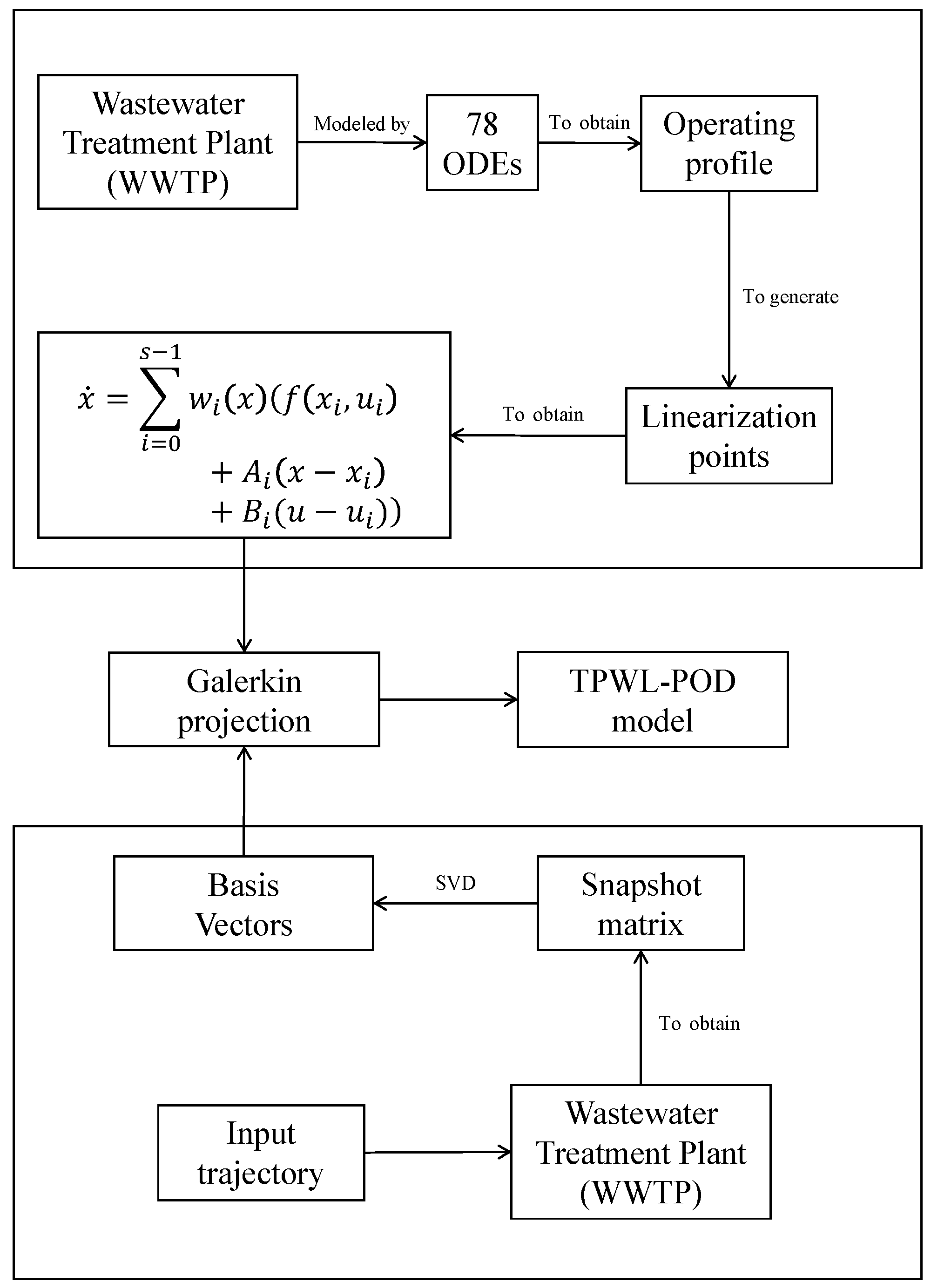
The generation of the reduced order TPWL-POD model consists of two parts: generation of the POD reduced basis and the generation of trajectory piecewise linear model. Figure 2 shows the methodology used in this work.

The strategy to generate the POD basis for WWTP process is described by Algorithm 4.

The strategy to generate the piecewise linear model is the same as the one shown in Section 3.2. After generating the linearization points $x_i$, these linearization points are projected to the reduced-order space, i.e., $z_i=U_k^T{x}_i$. The weighting parameter $w_i\left(z\right)$ is computed based on the states in reduced-order space, and the strategy to calculate it is the same as the steps in Algorithm 3.

Algorithm 4: Generation of POD basis algorithm

Simulate the nonlinear system for $t\in (0,N]$ to generate the snapshot matrix of the process, i.e., X. Take singular value decomposition on snapshot matrix X, $X=U\Sigma V^T$. Determine the proper reduced order k to choose the k most relevant basis vectors of the system. Generate the POD basis vectors matrix $U_k$.

5. Centralized EMPC Design Based on TPWL Model and TPWL-POD Model

In this section, we present the proposed centralized EMPC design based on two different models. The two considered models are as follows: TPWL model introduced in Section 3 and TPWL-POD model introduced in Section 4. The control objective is to minimize the economic cost introduced in Section 2.3.

5.1. Centralized EMPC Design Based on TPWL Model

First, the nonlinear model of the WWTP system is linearized using the trajectory piecewise linearization method proposed in Section 3. The EMPC developed based on the TPWL model can be formulated as the following optimization problem:

$$\begin{array}{cc}\hfill & u^{\ast }\left(\tau \right|t_k)=\arg \underset{u\left(\tau \right)\in S\left(\mathsf{\Delta }\right)}{\min }{\int }_{t_k}^{t_{k+N}}l\left(\tilde{x}\left(\tau \right),u\left(\tau \right)\right)d\tau \hfill \end{array}$$

(34a)

$$\begin{array}{cc}\hfill & \mathrm{s}.\mathrm{t}.\dot{\tilde{x}}\left(\tau \right)=\sum _{i=0}^{s-1}{w}_i\left(\tilde{x}\left(\tau \right)\right)(f(x_i,u_i)+A_i(\tilde{x}\left(\tau \right)-x_i)+B_i(u\left(\tau \right)-u_i))\hfill \end{array}$$

(34b)

$$\begin{array}{cc}\hfill & \tilde{x}\left(t_k\right)=x\left(t_k\right)\hfill \end{array}$$

(34c)

$$\begin{array}{cc}\hfill & u\left(\tau \right)\in \mathbb{U}\hfill \end{array}$$

(34d)

In the above optimization problem of Equation (34), $u^{\ast }\left(\tau \right|t_k)$ is the optimal solution to the problem. Equation (34a) denotes the objective function for the centralized EMPC controller that minimizes the economic cost l defined in Equation (17), N denotes the control horizon, and $S_i\left(\delta \right)$ represents a family of piecewise-constant functions. Equation (34b) is the approximated piecewise linear model of the nonlinear system as introduced in Section 3. The state measurement value at current sampling time $t_k$ (i.e., $x\left(t_k\right)$) is used to initialize the predicted state trajectory in Equation (34c). Equation (34d) is the constraint on input u.

The optimal input trajectory is achieved after the optimization problem Equation (34) is solved (i.e., $u^{\ast }\left(\tau \right|t_k)$). The first step value of the input trajectory is defined to be the manipulated input applied to the operating process at time instant $t_k$, which can be shown as follows:

$$\begin{array}{c}\hfill u\left(t\right)=u^{\ast }\left(t\right|t_k),t\in \left[t_k,t_{k+1}\right)\end{array}$$

(35)

5.2. Centralized EMPC Design Based on TPWL-POD Model

In this section, the centralized EMPC is designed based on the TPWL-POD model. The model is linearized using TPWL method shown in Section 3 and the order of the nonlinear system is reduced using POD method proposed in Section 4. The proposed EMPC design can be shown as follows:

$$\begin{array}{cc}\hfill & u^{\ast }\left(\tau \right|t_k)=\arg \underset{u\left(\tau \right)\in S\left(\mathsf{\Delta }\right)}{\min }{\int }_{t_k}^{t_{k+N}}l\left(U_{k}z\left(\tau \right),u\left(\tau \right)\right)d\tau \hfill \end{array}$$

(36a)

$$\begin{array}{cc}\hfill & \mathrm{s}.\mathrm{t}.\dot{\tilde{z}}\left(\tau \right)=\sum _{i=0}^{s-1}{w}_i\left(z\right)(A_{ir}z+B_{ir}u+{\gamma }_{ir})\hfill \end{array}$$

(36b)

$$\begin{array}{cc}\hfill & \tilde{z}\left(t_k\right)=U_k^{T}x\left(t_k\right)\hfill \end{array}$$

(36c)

$$\begin{array}{cc}\hfill & A_{ir}=U_k^T{A}_i{U}_k\hfill \end{array}$$

(36d)

$$\begin{array}{cc}\hfill & B_{ir}=U_k^T{B}_i\hfill \end{array}$$

(36e)

$$\begin{array}{cc}\hfill & {\gamma }_{ir}=U_k^T(f(x_i,u_i)-A_i{x}_i-B_i{u}_i)\hfill \end{array}$$

(36f)

$$\begin{array}{cc}\hfill & \sum _{i=0}^{s-1}{w}_i\left(z\right)=1\hfill \end{array}$$

(36g)

$$\begin{array}{cc}\hfill & u\left(\tau \right)\in \mathbb{U}\hfill \end{array}$$

(36h)

In the optimization problem of Equation (36), let $u^{\ast }\left(\tau \right|t_k)$ accounts for the optimal solution to this problem. The objective function is Equation (36a). Equation (36b) denotes the order reduced linear model using TPWL-POD method introduced in Section 4 for the nonlinear system. $A_{ir}$, $B_{ir}$, ${\gamma }_{ir}$, and $w_i\left(z\right)$ in model Equation (36b) are shown in Equations (36d)–(36g), respectively. In Equation (36c), the predicted state in the reduced-order space is initialized with the state measurement $x\left(t_k\right)$ and it is projected to the reduced-order space by multiplying the projection matrix $U_k$. Equation (36h) is the input constraint. The manipulated input applied to the control process is the first step value of the optimal input trajectory, i.e., $u^{\ast }\left(t\right|t_k),t\in \left[t_k,t_{k+1}\right)$.

6. Simulation Results

In this section, we apply the TPWL method introduced in Section 3 and the TPWL-POD method introduced in Section 4 to the WWTP. The reduced order basis and the linearization points for both TPWL model and TPWL-POD model are obtained based on a given training input signal. The approximated model accuracy for the nonlinear system with TPWL model and TPWL-POD model are discussed. We apply the proposed control strategies introduced in Section 5.1 and Section 5.2 to the modified BSM1 model. The performance of these control strategies is compared in terms of effluent quality, operating cost and computational efficiency under dry weather condition. The simulations are all carried out with a computing server with 2.0 GHz CPUs and the EMPC optimization problems are solved using interior point optimizer.

6.1. Simulation Settings

The dry weather condition data file are provided in the International Water Association Web site [40]. The inlet flowrate $Q_0$, and the concentration $Z_0$ of the influent flow can be found in the data file. The wastewater treatment plant is simulated with the average value of $Q_0$ and $Z_0$ under dry weather condition to achieve the optimal steady state. We consider the optimal steady state as the initial condition for this wastewater treatment process.

To compare the performance index between different control strategies, the simulation time is set to be 14 days and the simulation results of the last 7 days will be used to evaluate the control performance index. The sampling time is picked as $\mathsf{\Delta }=15$ min.

The weighting parameter $\beta$ in Algorithm 3 is set to be 25. The weighting coefficients ${\alpha }_{EQ}$ and ${\alpha }_{OCI}$ in the economic control objective function Equation (17) are considered to be 1 and 0.3. The control horizon is determined to be 25 in all EMPC controller designs. The constraints on manipulated inputs (i.e., $\mathbb{U}$) for all control designs are considered as follows:

$$\begin{array}{cc}\hfill 0& \le Q_a\le 5Q_{0,\mathrm{stab}}\hfill \end{array}$$

(37)

$$\begin{array}{cc}\hfill 0& \le K_L{a}_5\le 240\mathrm{d}\mathrm{a}{\mathrm{y}}^{-1}\hfill \end{array}$$

(38)

where $Q_{0,\mathrm{stab}}$ is the average dry weather influent flow rate and is equal to 18,446 ${\mathrm{m}}^3/\mathrm{day}$.

6.2. Model Validation and Comparison

6.2.1. Model Validation

To verify the generated TPWL model and TPWL-POD model not only work for the inputs which are very close to the given training input but also for other inputs, the accuracy of the model is investigated under different manipulated input values. For model validation, the number of linearization points s in both TPWL model and TPWL-POD model is set to be 9, and the reduced basis order k is set to be 35 for TPWL-POD model. Note that the number of linearzation points s and the order k are determined based on extensive simulations. The guideline is to achieve a balance between model accuracy and evaluation time. In general, with the increase of s and k, the accuracy of the model increases but the time needed in evaluation also increases. When determining s and k, we need to achieve a balance between accuracy and evaluation time, which is indeed case specific.

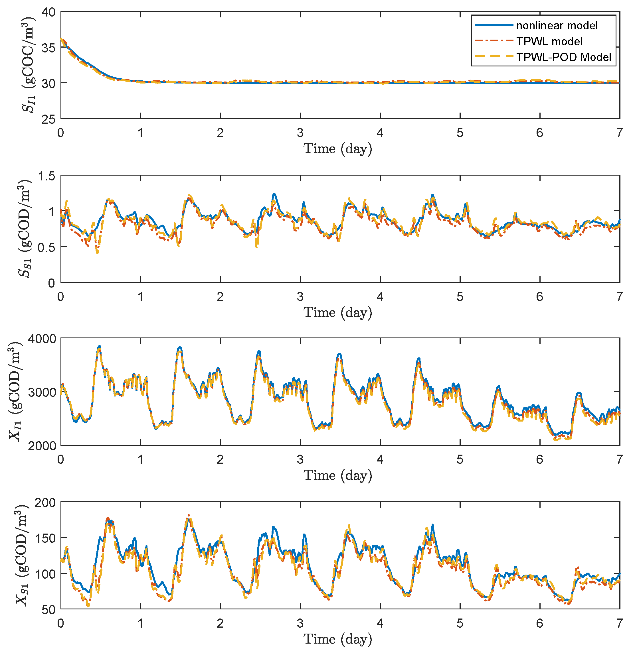
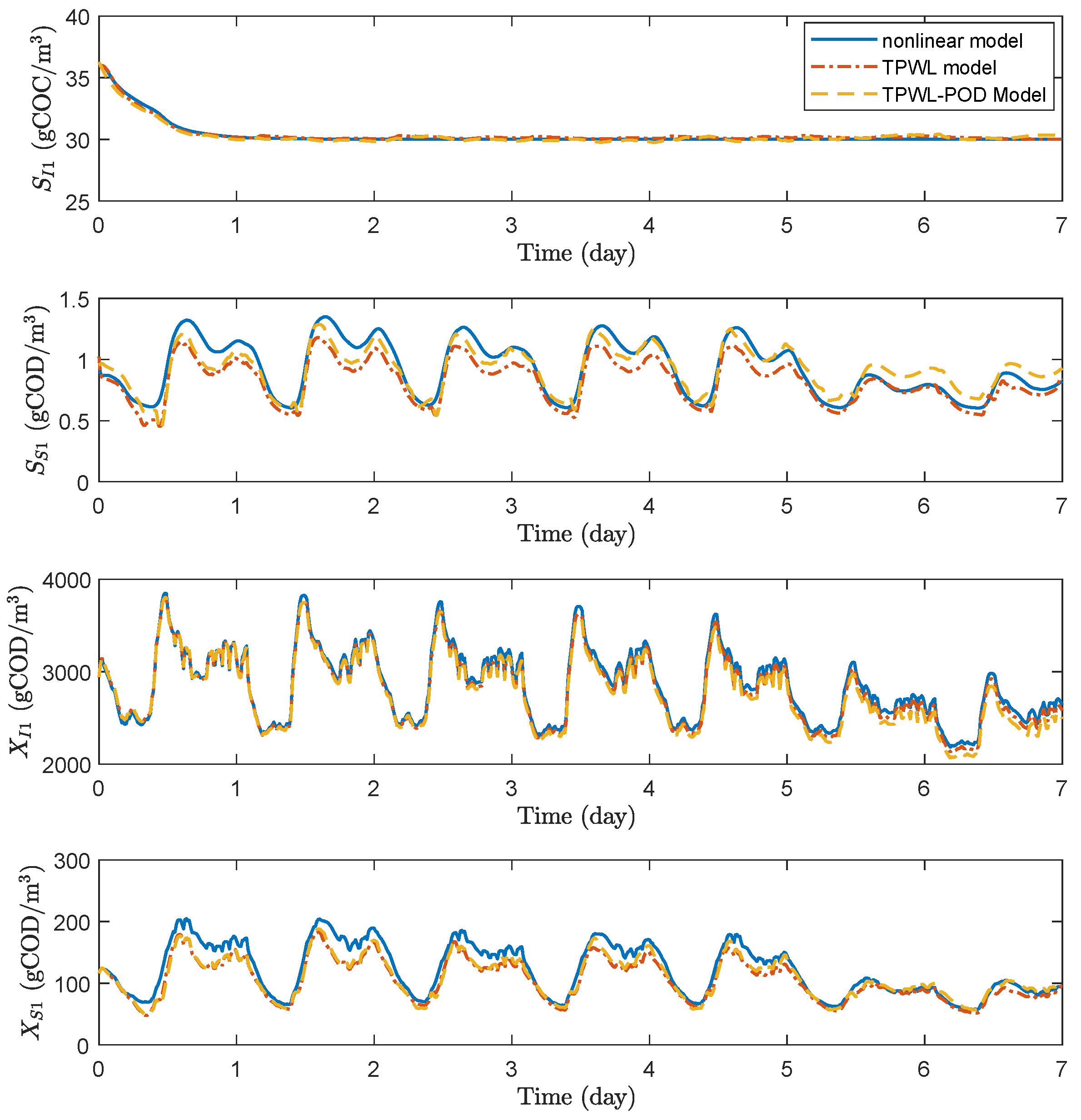
The approximated state trajectories based on TPWL model, TPWL-POD model and the actual state trajectories based on the nonlinear system model for certain process states in the first week of the operation under the training input signal and fixed input signal are presented in Figure 3 and Figure 4, respectively. For the fixed input signal, the two manipulated inputs are fixed as $K_L{a}_5=83.9405$${\mathrm{d}}^{-1}$ and $Q_a$ = 37,723.4072 ${\mathrm{m}}^3/\mathrm{day}$. As can be seen from Figure 3 and Figure 4, the state trajectories almost overlap each other in all the cases. The results show that TPWL model and TPWL-POD model provide accurate models for the original nonlinear WWTP system.

6.2.2. Model Comparison

The model approximation accuracy and computation time for TPWL method and TPWL-POD method are investigated under different number of the linearization points (s).

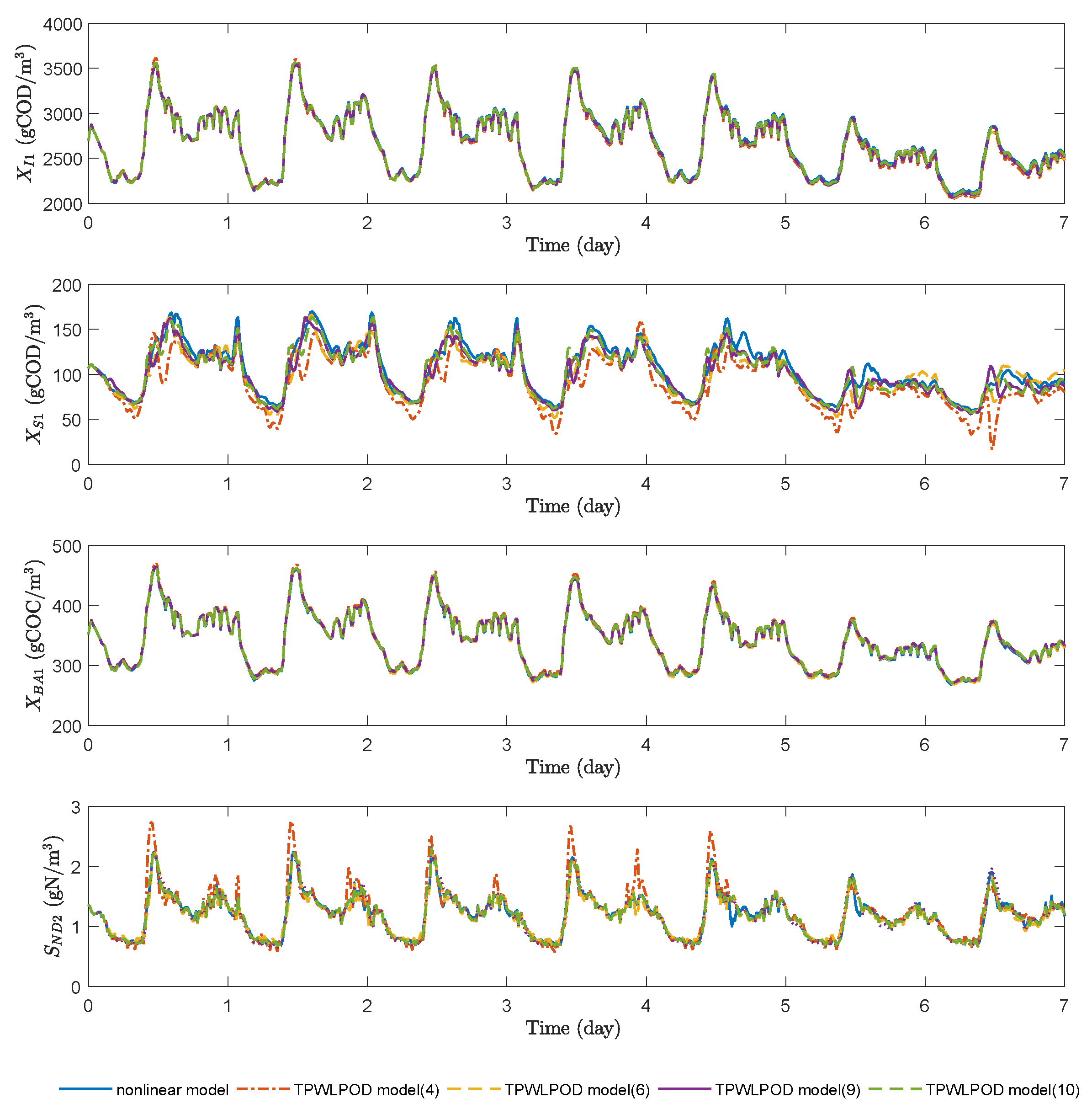
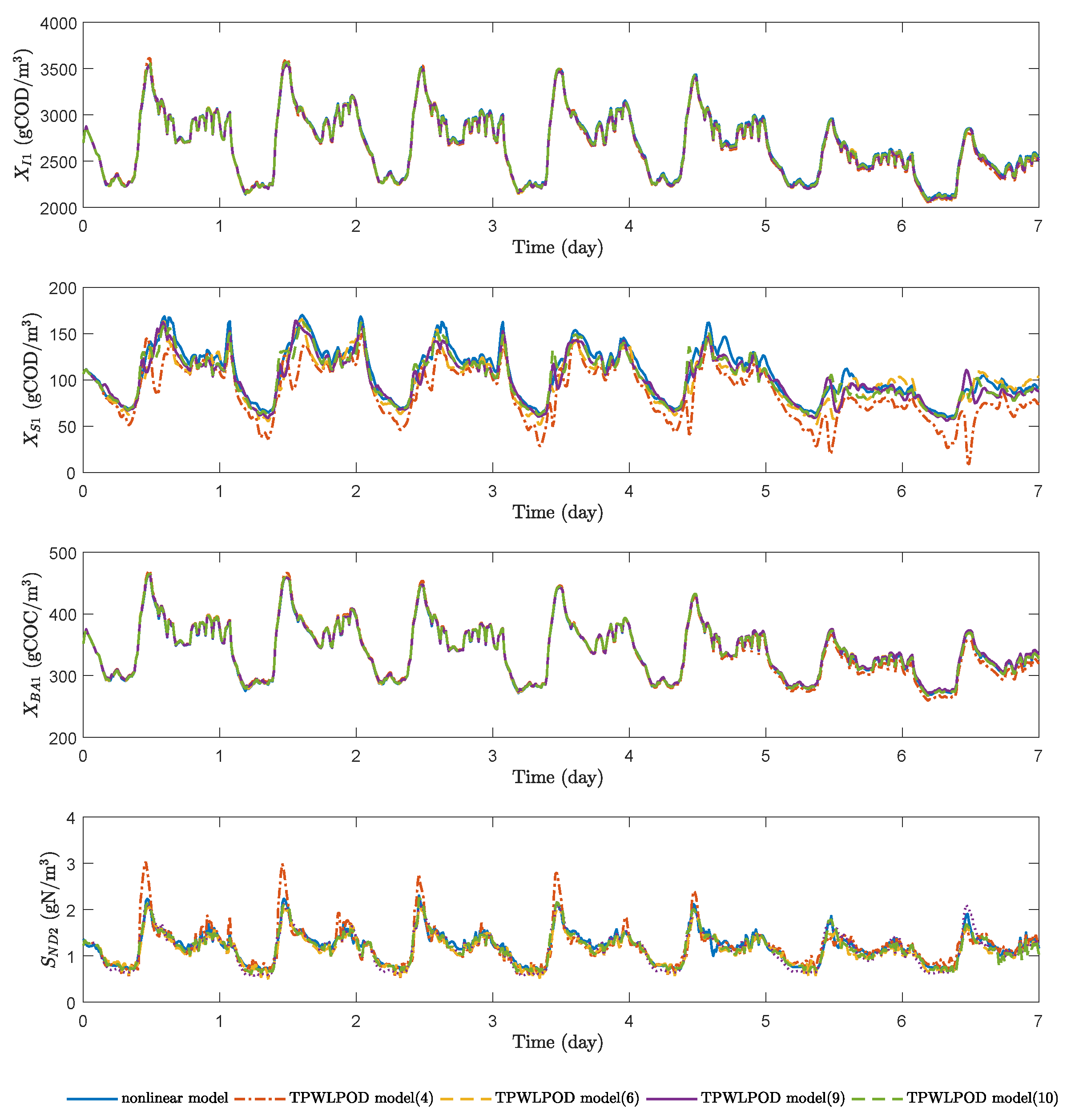
Figure 5 presents the state trajectories for certain process states using TPWL model with different number of linearization points under a given input signal in dry weather condition. Figure 6 shows the state trajectories for those states using TPWL-POD model with different number of linearization points under the same input signal in dry weather condition.

Table 4. Root mean square error of TPWL model and TPWL-POD model with different number of the linearization points.

Threshold $\mathit{\delta }$	Linearization Point Number	RMSE TPWL Model	RMSE TPWL-POD Model
1000	4	18.3979	48.6197
950	6	10.5667	12.4511
600	9	6.0770	8.6849
570	10	5.5003	6.5913

presents the root mean square error of TPWL model and TPWL-POD model with different number of the linearization points. The result elucidates that the approximated model accuracy would increase as the number of linearization points increase for both TPWL and TPWL-POD models. As can be seen from the table, under the same linearization point number, TPWL model provides a better approximation than TPWL-POD model.

6.3. Simulation Results of EMPC in Dry Weather

We evaluate the performance of EMPC based on the nonlinear model, EMPC based on TPWL model and EMPC based on TPWL-POD model in dry weather condition, respectively.

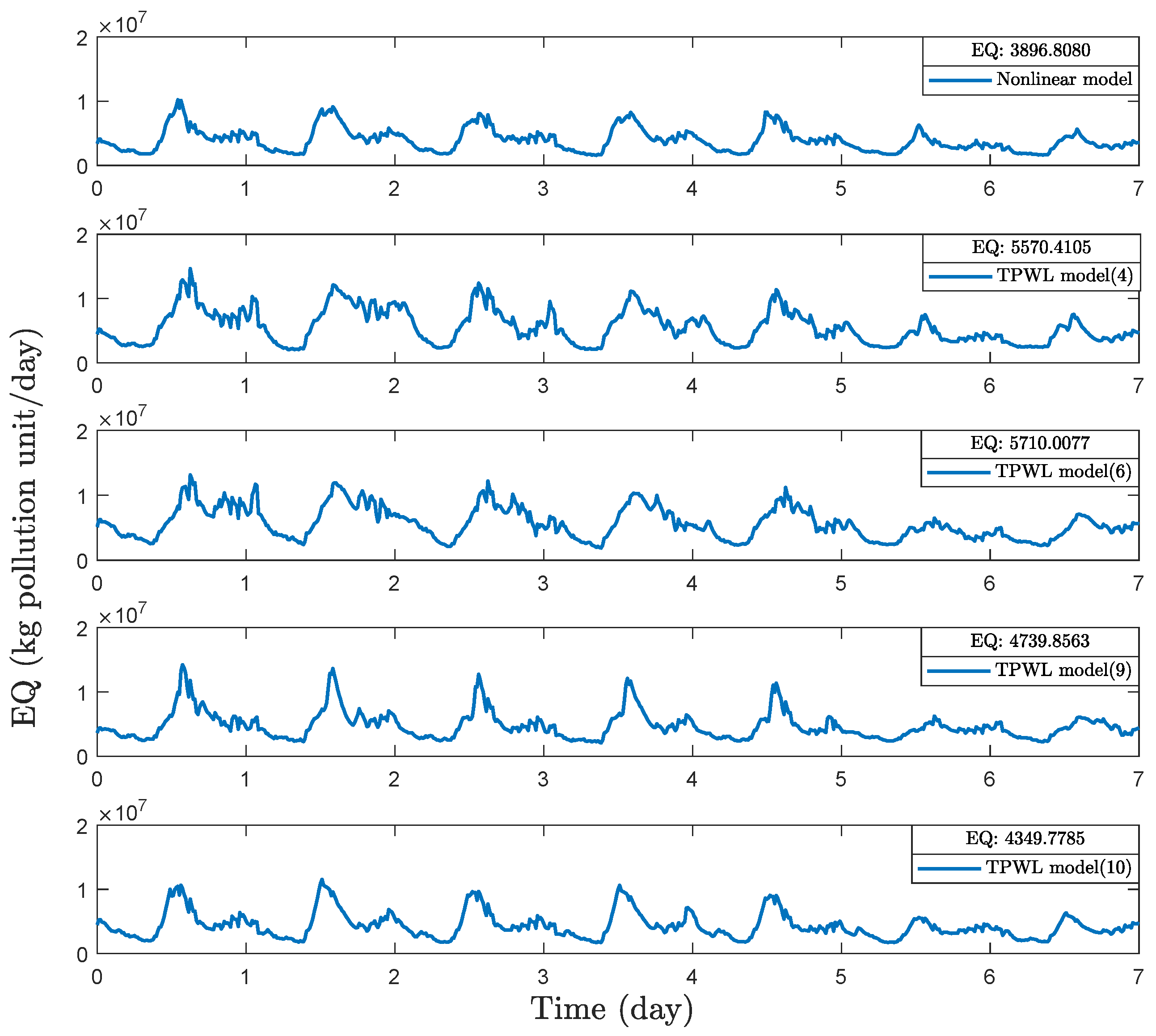
To study the impacts of the number of linearization points (s) on EMPC design based on TPWL model, we apply the proposed EMPC scheme with $s=4$, $s=6$, $s=9$, and $s=10$ respectively. The trajectories of the instantaneous effluent quality level in dry weather condition under EMPC based on the nonlinear model, EMPC based on TPWL model with linearization point number $s=4$, $s=6$, $s=9$, $s=10$ are presented in Figure 7.

Table 5. Control performance in dry weather condition under EMPC based on nonlinear model, TPWL model with different linearization point numbers ($s=4$, $s=6$, $s=9$, $s=10$).

Model	Linearization Point Number	Average Computation Time (s)	EQ (kg Pollution Unit/Day)	OCI	Average Performance Cost
Nonlinear	N/A	$7.34\times {10}^4$	3896.8080	19,592.3016	9774.4985
TPWL	4	$5.13\times {10}^4$	5570.4105	19,958.9991	11,558.1102
	6	$5.28\times {10}^4$	5710.0077	19,404.2978	11,531.2970
	9	$5.72\times {10}^4$	4739.8563	19,654.6556	10,636.2530
	10	$8.53\times {10}^4$	4349.7785	20,014.8107	10,354.2217

presents the calculated control performance index EQ, OCI, average economic cost, and average evaluation time consumed over the full operating period for EMPC based on nonlinear model and EMPC based on TPWL model with $s=4$, $s=6$, $s=9$, $s=10$. Based on the average EQ value shown in Table 5 and the instantaneous effluent quality level shown in Figure 7, we can conclude that the effluent quality level is improved as the linearization point number s in TPWL model increases. Our objective is to minimize the average economic cost. Consequently, the smaller average performance cost indicates that the model can give us a better control performance. As can be seen from Table 5, the EMPC with nonlinear model provides us with the best control performance, and the control performance of EMPC based on TPWL model enhances as the linearization point number raises. The EMPC based on TPWL model with $s=4$ performs $18.24\%$ worse than nonlinear model while the EMPC based on TPWL model with $s=10$ is only $5.93\%$ lower than nonlinear model. As the linearization point number s increases from 4 to 10, the control performance improves $10.42\%$.

To compare the evaluation times of EMPC based on the nonlinear model and EMPC based on TPWL model with $s=4$, $s=6$, $s=9$, $s=10$, the average computation time consumed over the full operation period is evaluated and shown in Table 5. The average computation time over the full operation period is evaluated based on 10 repetitive simulation runs. The evaluation time consumed by EMPC based on TPWL model with $s=4$, $s=6$, and $s=9$ is $30.02\%$, $27.97\%$, and $22.05\%$ less than EMPC based on nonlinear model, respectively. However, as the linearization point number s increases, the computation load increases accordingly. The EMPC based on TPWL model with $s=10$ is $16.29\%$ lower than EMPC with the nonlinear model.

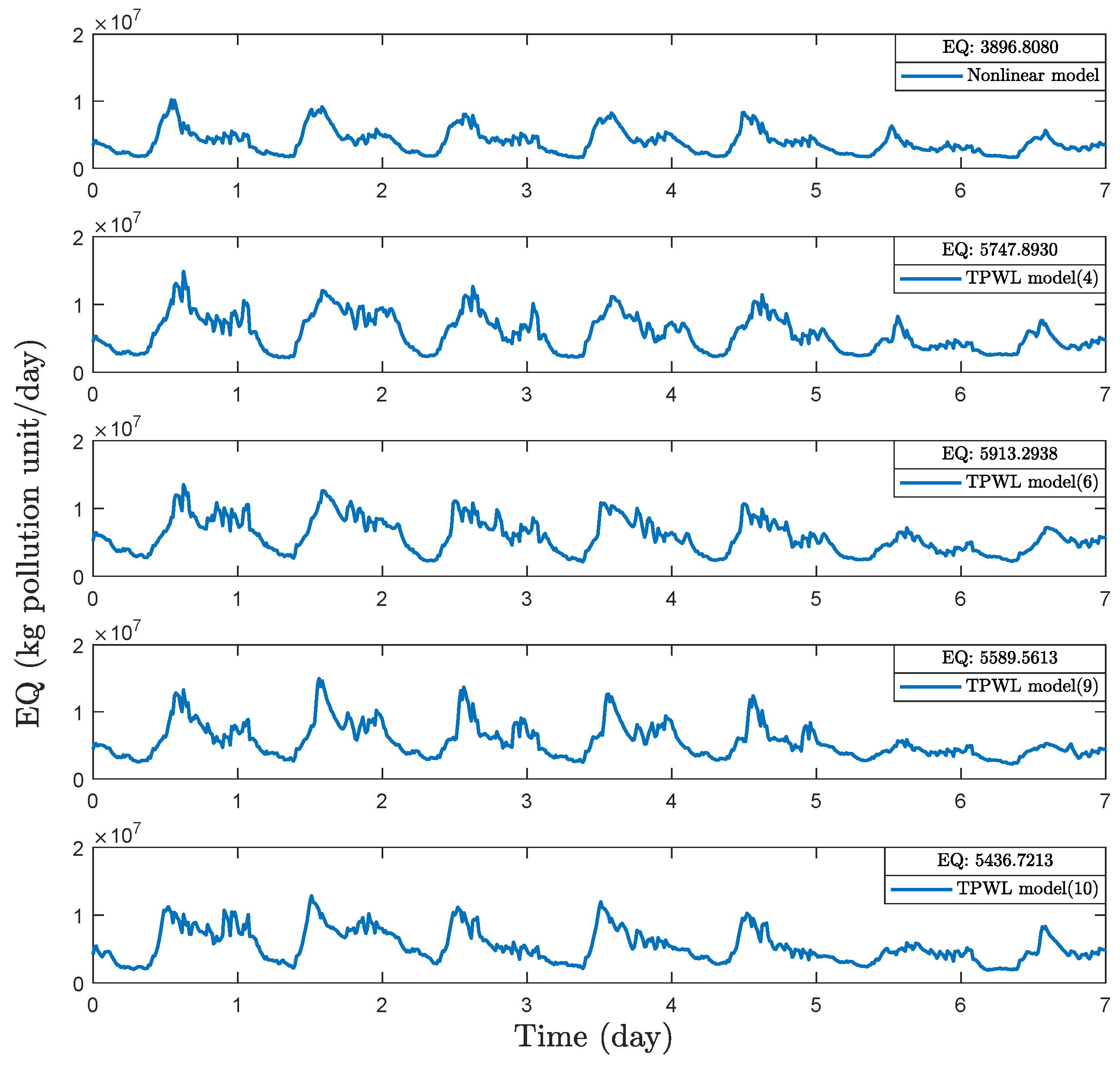
We also evaluate how linearization point number s influences the control performance of EMPC based on TPWL-POD model. Figure 8 presents the trajectories of the instantaneous effluent quality level in dry weather condition under EMPC based on the nonlinear model, EMPC based on TPWL-POD model with linearization point number $s=4$, $s=6$, $s=9$, $s=10$.

Table 6. Control performance in dry weather condition under EMPC based on nonlinear model, TPWL-POD model with different linearization point numbers ($s=4$, $s=6$, $s=9$, $s=10$).

Model	Linearization Point Number	Average Computation Time (s)	EQ (kg Pollution Unit/Day)	OCI	Average Performance Cost
Nonlinear	N/A	$7.34\times {10}^4$	3896.8080	19,592.3016	9774.4985
TPWL-POD	4	$2.19\times {10}^4$	5747.8930	19,902.6197	11,718.6789
	6	$2.39\times {10}^4$	5913.2938	19,378.8133	11,726.9378
	9	$3.34\times {10}^4$	5589.5613	19,328.1781	11,388.0147
	10	$6.19\times {10}^4$	5436.7213	19,280.6409	11,220.9136

shows the EQ, OCI, average economic cost and average evaluation time of EMPC based on nonlinear model, EMPC based on TPWL-POD model with $s=4$, $s=6$, $s=9$ and $s=10$. We can draw the same conclusion as we have for EMPC based on TPWL model. The more linearization points we consider, the better control performance of EMPC based on TPWL-POD model would be. The average evaluation time consumed by TPWL-POD model will raise when the linearization point number s increases. Compared with the evaluation time consumed by EMPC based on the nonlinear model, EMPC based on TPWL-POD model with $s=4$, $s=6$, $s=9$ and $s=10$ is 70.13%, 67.40%, 54.51% and 15.62% less, respectively.

By examining Table 5 and Table 6, we can see that with the same linearization point number s, the average evaluation time used by EMPC based on TPWL-POD model is approximately 58.54% less than that based on the TPWL model. The average evaluation time of the EMPC based on TPWL-POD model is up to 70.13% lower than EMPC based on the nonlinear model. However, it should be noted that the control performance for EMPC based on TPWL-POD model is degraded by 1.39% compared with the TPWL model and 19.89% compared with the original nonlinear model.

7. Conclusions

Two model approximation methods are applied to the modified nonlinear WWTP process. In particular, the two model approximation methods are TPWL method and TPWL-POD method. Two centralized EMPC controllers are designed based on the two models correspondingly. We have compared the model accuracy of the TPWL model and the TPWL-POD model with nonlinear model. In this work, our main objective was to investigate how the computational efficiency of EMPC may be improved through model reduction and approximation. While the investigated methods lead to improved computational efficiency, it does come at the cost of reduced control performance. In the future work, we will study how to improve the computational efficiency while remain the control performance close to the one when the original nonlinear model is used.

References

1. Zhang, A.; Yin, X.; Liu, S.; Zeng, J.; Liu, J. Distributed economic model predictive control of wastewater treatment plants. Chem. Eng. Res. Des. 2019, 141, 144–155. [Google Scholar] [CrossRef]
2. Alex, J.; Benedetti, L.; Copp, J.; Gernaey, K.V.; Jeppsson, U.; Nopens, I.; Pons, M.N.; Rieger, L.; Rosen, C.; Steyer, J.P.; et al. Benchmark Simulation Model No. 1 (BSM1); Technical Report; Department of Industrial Electrical Engineering and Automation, Lund University: Lund, Sweden, 2008. [Google Scholar]
3. Machado, V.C.; Gabriel, D.; Lafuente, J.; Baeza, J.A. Cost and effluent quality controllers design based on the relative gain array for a nutrient removal WWTP. Water Res. 2009, 43, 5129–5141. [Google Scholar] [CrossRef] [PubMed]
4. Tzoneva, R. Optimal PID control of the dissolved oxygen concentration in the wastewater treatment plant. In Proceedings of the AFRICON 2007, Windhoek, South Africa, 26–28 September 2007; pp. 1–7. [Google Scholar]
5. Gutierrez, G.; Ricardez-Sandoval, L.A.; Budman, H.; Prada, C. An MPC-based control structure selection approach for simultaneous process and control design. Comput. Chem. Eng. 2014, 70, 11–21. [Google Scholar] [CrossRef]
6. Rafiei-Shishavan, M.; Mehta, S.; Ricardez-Sandoval, L.A. Simultaneous design and control under uncertainty: A back-off approach using power series expansions. Comput. Chem. Eng. 2017, 99, 66–81. [Google Scholar] [CrossRef]
7. Rodríguez-Pérez, B.E.; Flores-Tlacuahuac, A.; Ricardez-Sandoval, L.; Lozano, F.J. Optimal water quality control of sequencing batch reactors under uncertainty. Ind. Eng. Chem. Res. 2018, 57, 9571–9590. [Google Scholar] [CrossRef]
8. Francisco, M.; Vega, P.; Revollar, S. Model predictive control of BSM1 benchmark of wastewater treatment process: A tuning procedure. In Proceedings of the 50th IEEE Conference on Decision and Control and European Control Conference (CDC-ECC), Orlando, FL, USA, 12–15 December 2011; pp. 7057–7062. [Google Scholar]
9. Holenda, B.; Domokos, E.; Rédey, Á.; Fazakas, J. Dissolved oxygen control of the activated sludge wastewater treatment process using model predictive control. Comput. Chem. Eng. 2008, 32, 1270–1278. [Google Scholar] [CrossRef]
10. Han, H.G.; Qiao, J.F.; Chen, Q.L. Model predictive control of dissolved oxygen concentration based on a self-organizing RBF neural network. Control Eng. Pract. 2012, 20, 465–476. [Google Scholar] [CrossRef]
11. Shen, W.; Chen, X.; Corriou, J.P. Application of model predictive control to the BSM1 benchmark of wastewater treatment process. Comput. Chem. Eng. 2008, 32, 2849–2856. [Google Scholar] [CrossRef]
12. Ostace, G.S.; Cristea, V.M.; Agachi, P.Ş. Cost reduction of the wastewater treatment plant operation by MPC based on modified ASM1 with two-step nitrification/denitrification model. Comput. Chem. Eng. 2011, 35, 2469–2479. [Google Scholar] [CrossRef]
13. O’Brien, M.; Mack, J.; Lennox, B.; Lovett, D.; Wall, A. Model predictive control of an activated sludge process: A case study. Control Eng. Pract. 2011, 19, 54–61. [Google Scholar] [CrossRef]
14. Zeng, J.; Liu, J. Economic model predictive control of wastewater treatment processes. Ind. Eng. Chem. Res. 2015, 54, 5710–5721. [Google Scholar] [CrossRef]
15. Nevistić, V.; Morari, M. Constrained control of feedback-linearizable systems. In Proceedings of the 3rd European Control Conference ECC95, Roma, Italy, 5–8 Semptember 1995; pp. 1726–1731. [Google Scholar]
16. Garcia, C.E. Quadratic dynamic matrix control of nonlinear processes. An application to a batch reactor process. In Proceedings of the AIChE Annual Meeting, San Francisco, CA, USA, 25–30 November 1984. [Google Scholar]
17. Gattu, G.; Zafiriou, E. Nonlinear quadratic dynamic matrix control with state estimation. Ind. Eng. Chem. Res. 1992, 31, 1096–1104. [Google Scholar] [CrossRef] [Green Version]
18. Lee, J.H.; Ricker, N.L. Extended Kalman Filter Based Nonlinear Model Predictive Control. Ind. Eng. Chem. Res. 1994, 33, 1530–1541. [Google Scholar] [CrossRef]
19. De Oliveira, S.L. Model Predictive Control (MPC) for Constrained Nonlinear Systems. Ph.D. Thesis, California Institute of Technology, Pasadena, CA, USA, 1996. [Google Scholar]
20. Nevistić, V. Constrained Control of Nonlinear Systems. Ph.D. Thesis, ETH Zurich, Zurich, Switzerland, 1997. [Google Scholar]
21. Zheng, A. A computationally efficient nonlinear MPC algorithm. In Proceedings of the American Control Conference, Albuquerque, NM, USA, 6 June 1997; pp. 1623–1627. [Google Scholar]
22. Zheng, A. Nonlinear model predictive control of the Tennessee Eastman process. In Proceedings of the 1998 American Control Conference, Philadelphia, PA, USA, 26 June 1998; pp. 1700–1704. [Google Scholar]
23. Xie, W.; Bonis, I.; Theodoropoulos, C. Off-line model reduction for on-line linear MPC of nonlinear large-scale distributed systems. Comput. Chem. Eng. 2011, 35, 750–757. [Google Scholar] [CrossRef]
24. Marquez, A.; Oviedo, J.J.; Odloak, D. Model Reduction Using Proper Orthogonal Decomposition and Predictive Control of Distributed Reactor System. J. Control Sci. Eng. 2013, 2013, 1–19. [Google Scholar] [CrossRef] [Green Version]
25. Leibfritz, F.; Volkwein, S. Reduced order output feedback control design for PDE systems using proper orthogonal decomposition and nonlinear semidefinite programming. Linear Algebra Appl. 2006, 415, 542–575. [Google Scholar] [CrossRef]
26. Hömberg, D.; Volkwein, S. Control of laser surface hardening by a reduced-order approach using proper orthogonal decomposition. Math. Comput. Model. 2003, 38, 1003–1028. [Google Scholar] [CrossRef]
27. Ly, H.V.; Tran, H.T. Modeling and control of physical processes using proper orthogonal decomposition. Math. Comput. Model. 2001, 33, 223–236. [Google Scholar] [CrossRef] [Green Version]
28. Atwell, J.A.; King, B.B. Proper orthogonal decomposition for reduced basis feedback controllers for parabolic equations. Math. Comput. Model. 2001, 33, 1–19. [Google Scholar] [CrossRef]
29. Padhi, R.; Balakrishnan, S.N. Proper orthogonal decomposition based optimal neurocontrol synthesis of a chemical reactor process using approximate dynamic programming. Neural Netw. 2003, 16, 719–728. [Google Scholar] [CrossRef]
30. Yin, X.; Liu, J. State estimation of wastewater treatment plants based on model approximation. Comput. Chem. Eng. 2018, 111, 79–91. [Google Scholar] [CrossRef]
31. Lao, L.; Ellis, M.; Christofides, P.D. Economic model predictive control of parabolic PDE systems: Addressing state estimation and computational efficiency. J. Process Control 2014, 24, 448–462. [Google Scholar] [CrossRef]
32. Lao, L.; Ellis, M.; Christofides, P.D. Economic Model Predictive Control of Transport-Reaction Processes. Ind. Eng. Chem. Res. 2014, 53, 7382–7396. [Google Scholar] [CrossRef]
33. Rewienski, M.; White, J. A trajectory piecewise-linear approach to model order reduction and fast simulation of nonlinear circuits and micromachined devices. IEEE Trans. Comput.-Aided Des. Integr. Circ. Syst. 2003, 22, 155–170. [Google Scholar] [CrossRef]
34. Busch, J.; Elixmann, D.; Kühl, P.; Gerkens, C.; Schlöder, J.P.; Bock, H.G.; Marquardt, W. State estimation for large-scale wastewater treatment plants. Water Res. 2013, 47, 4774–4787. [Google Scholar] [CrossRef] [PubMed]
35. Henze, M.; Grady, C.P.L.; Gujer, W.; Marais, G.V.R.; Matsuo, T. A general model for single-sludge wastewater treatment systems. Water Res. 1987, 21, 505–515. [Google Scholar] [CrossRef] [Green Version]
36. Zeng, J.; Liu, J.; Zou, T.; Yuan, D. State estimation of wastewater treatment processes using distributed extended Kalman filters. In Proceedings of the 2016 IEEE 55th Conference on Decision and Control (CDC), Las Vegas, NV, USA, 12–14 December 2016; pp. 6721–6726. [Google Scholar]
37. Vanrolleghem, P.A.; Jeppsson, U.; Carstensen, J.; Carlssont, B.; Olsson, G. Integration of wastewater treatment plant design and operation-a systematic approach using cost functions. Water Sci. Technol. 1996, 34, 159–171. [Google Scholar] [CrossRef]
38. Antoulas, A.C. Approximation of Large-Scale Dynamical Systems: An Overview. IFAC Proc. Vol. 2004, 37, 19–28. [Google Scholar] [CrossRef] [Green Version]
39. Chatterjee, A. An introduction to the proper orthogonal decomposition. Curr. Sci. 2000, 78, 808–817. [Google Scholar]
40. International Water Association. Available online: http://www.benchmarkwwtp.org (accessd on 2 January 2019).
Figure 1. A schematic of the wastewater treatment plant.
Processes 07 00682 g001
Figure 2. TPWL-POD framework.
Processes 07 00682 g002
Figure 3. Trajectories of the states based on nonlinear model (blue solid lines), TPWL model (red dash-dot lines), TPWL-POD model (yellow dashed lines) under training input signal in dry weather.
Processes 07 00682 g003
Figure 4. Trajectories of the states based on nonlinear model (blue solid lines), TPWL model (red dash-dot lines), TPWL-POD model (yellow dashed lines) under fixed input signal in dry weather.
Processes 07 00682 g004
Figure 5. Trajectories of the states based on nonlinear model (blue solid lines), TPWL model with 4 linearization points (red dash-dot lines), TPWL model with 6 linearization points (yellow dashed lines), TPWL model with 9 linearization points (purple solid lines), and TPWL model with 10 linearization points (green dashed lines) under a given input signal in dry weather.
Processes 07 00682 g005
Figure 6. Trajectories of the states based on nonlinear model (blue solid lines), TPWL-POD model with 4 linearization points (red dash-dot lines), TPWL-POD model with 6 linearization points (yellow dashed lines), TPWL-POD model with 9 linearization points (purple solid lines), and TPWL-POD model with 10 linearization points (green dashed lines) under a given input signal in dry weather.
Processes 07 00682 g006
Figure 7. Trajectories of the instantaneous effluent quality level in dry weather condition under EMPC based on nonlinear model, TPWL model with 4 linearization points, TPWL model with 6 linearization points, TPWL model with 9 linearization points and TPWL model with 10 linearization points.
Processes 07 00682 g007
Figure 8. Trajectories of the instantaneous effluent quality level in dry weather condition under EMPC based on nonlinear model, TPWL-POD model with 4 linearization points, TPWL-POD model with 6 linearization points, TPWL-POD model with 9 linearization points and TPWL-POD model with 10 linearization points.
Processes 07 00682 g008