Simulation of Ion Exchange Resin with Finite Difference Methods

Zhu, Yawen; Liu, Bobo; Peng, Ruichao; Luo, Yunbai; Yu, Ping

doi:10.3390/pr7100675

Open AccessArticle

Simulation of Ion Exchange Resin with Finite Difference Methods

College of Chemistry & Molecular Sciences, Wuhan University, Wuhan 430072, China

^*

Author to whom correspondence should be addressed.

Processes 2019, 7(10), 675; https://doi.org/10.3390/pr7100675

Submission received: 23 August 2019 / Revised: 9 September 2019 / Accepted: 16 September 2019 / Published: 1 October 2019

(This article belongs to the Section Materials Processes)

Download

Browse Figures

Review Reports Versions Notes

Abstract

:

Ion exchange resin is used to remove potentially corrosive impurities from coolant in the first circuit of a nuclear power plant. After one operational cycle, the used and unused resin in the mixed bed is discarded as solid waste. The aim of this work is to create a mathematical model to predict the operational cycle time of the mixed bed resin for reducing unused resin discharge. A partial differential equation (PDE) was set up with the conservation of matter. A finite difference method was used to solve the PDE. Matlab was the programming and calculating tool used in this work. The data from solution were obtained at different time and space nodes. The model was then verified experimentally using different ions on exchange columns. Concentrations of K⁺, Mn²⁺, and Cl^- were calculated to verify the validation of the model by comparing it with experimental data. The calculated values showed good consistency with the experimental value.

Keywords:

ion exchange; finite difference method; simulation; Matlab

Graphical Abstract

1. Introduction

A chemical and volume control system is an auxiliary system in the first circuit of a nuclear power plant [1,2,3,4]. Its main function is to regulate the purity of coolant and to moderate mechanical stresses (such as pressure) on the circuit. Purification is achieved through the use of a mixture of cationic and anionic exchange resins in the fixed bed [5,6,7,8,9].

The ability to calculate breakthrough curves [10,11] for mixed bed ion exchange resins [12,13,14,15,16,17] (i.e., the relationship between running time and concentrations of pollutant ions that escape in the effluent) would be of great use in predicting the operational lifetimes of mixed-bed resins for nuclear reactors [18,19,20]. However, most of these models are limited because they are either difficult to solve or require too many dynamic parameters.

The first attempt at creating such a model was made in 1951, by J. B. Rosen of Oxford University [21]. Further work was done by Yi et al. [22], Ebrahimi. et al. [23], Xiu [24], and Wu et al. [25], who mainly based their models on equations for linear driving force and thin film diffusion [26,27] at low solute concentrations [28]. All of the above were typical models for predicting breakthrough curves, which provided some inspiration for this work.

Some of the models most commonly used today for modeling ion exchange are the Thomas (TH), Yoon–Nelson (YN), and Adams–Bohart (AB) [29,30] models. However, one common characteristic of all three models is that they produce a linear function that relates effluent concentration to running time. Further work by Kataoka [31,32] showed the influence of diffusion coefficient on computation. Lin, X. et al. [33], Aurélie et al. [34], Yang, J. et al. [35], and Murillo, R. et al. [36] also produced methods for modeling ion exchange. However, the concentration of the other position column, except outflow, could be calculated and are seldom mentioned.

In summary, all previous research has modeled ion exchange using an analytic method [37]. There are few studies that have attempted to model ion exchange using a finite difference method. Yi [22] and Jian Wu [25] used a finite difference method to solve an ion exchange model, and the difference compared to this work was that the complete derivation and discretization of the difference equation. The results of their work produced comprehensive computational data. The advantage of a finite difference method is that the results of the calculation are presented from two dimensions of time and space. A finite difference method requires much more computation than an analytical method, however the development of modern computers has solved this problem.

This work aims to use a finite difference method to produce a novel model for calculating breakthrough curves of ion exchange resins. Partial differential equations that describe changes in the concentration of effluent over time were derived using a differential element method. The partial differential equations (PDEs) were then solved using a finite difference method with controllable precision and good convergence. Calculation and data visualization were performed using Matlab. This model was then tested against experimental data and found to be in good agreement. The figures of data have intuitive visualization.

2. Modeling

2.1. Modeling Assumptions

The system is controlled entirely by film diffusion [4]. The selectivity coefficient is constant and independent of temperature. The reaction speed is instantaneous as compared to the exchange speed. Axial diffusion can be ignored. The whole flow process is plug flow [27]. All changes to the system are isothermal and isobaric. The resin is homogeneous. There is no net electrical current.

2.2. Equations

Wolfgang [38] provided new information about the combination of the Nernst–Planck equation [39,40] and convection equation. The basic idea of this method was to discretize the ordinary equation to get the difference scheme. The detailed derivative is shown in Appendix A.

2.3. Initial Condition

On the basis of the actual situation, the concentration value at the inlet of the column is the initial concentration of solution at any time. Obviously, there is no substance when the time value is zero. Thus, the initial conditions are:

C = C₀ for H = 0, t = 0,1,2,3…j

C = 0 for t = 0, H = 1,2,3…n

The initial conditions are discretized.

2.4. Numerical Method

When calculating these models, it is necessary to compare the actual data of the test with the existing article parameters, such as the length of the resin column, velocity, and initial concentration. In general, modeling the behavior of the ion exchange resin over time begins by substituting the initial conditions into the system of PDEs and then proceeds iteratively until the concentration values at all space and time nodes are obtained.

The selection of an appropriate time step and space node is very significant for successful calculation using this system. As mentioned above, a one-dimensional convection equation is solved using a finite difference method to yield an upwind difference scheme. Selection of the time step directly affects the results.

A program was created in Matlab that used a for loop structure to calculate the concentration data at different time nodes, which proved to be an effective way to carry out the iterative calculation. Unlike an analytic solution to the system of equations, this technique produced a matrix containing concentration values at all space and time nodes for the flow of material through the column.

3. Experiment

The nuclear grade purification resin (ZGNR8715) was provided by the ZhengGuang company. Its physical and chemical properties are listed in Table 1.

The experimental procedure is shown in Figure 1. Tests were conducted under controlled conditions of pressure and temperature. The breakthrough point was determined when the conductivity of effluent was 2 μs/cm. The water used in the experiment was ultrapure water filtered via reverse osmosis, electro-deionization, and a mixed bed ion resin purification column (separate from the resin being tested). The conductivity range of the ultrapure water was 0.06~0.16 µs/cm. A constant-speed pump was used to inject 3 × 10⁻⁴ mol/L solution of a given ion into the top of the column. The column was filled with 100 mL of resin. The effluent samples were then collected at intervals and analyzed using high performance ion chromatography.

4. Results and Discussion

4.1. Convergence of the Model

The validation of a model not only depends on the consistency but also relies on convergence. In the circumstance that the computation is stable, values that are too big or too small have an effect on accuracy. A smaller time step can make the result more precise but can also create a risk of non-convergence. Thus, exploring the effect of the time step value on model convergence is necessary. The effect of the interval value is shown in Figure 2.

The effect of the interval value is shown in Figure 2. When the dt value is 0.1 or 0.01, there are totally different computation curves. The blue line, in Figure 2, shows a good result, but the hot line with a value of 0.01 exhibits non-convergence. By constantly adjusting the time step, the most appropriate value is determined. In a complex iterative process, the value of the time interval needs to be accurate enough to make the result adaptable. One advantage of Matlab programming is that adjusting a parameter is really easy, which means the program can be debugged when the calculation result is not converged.

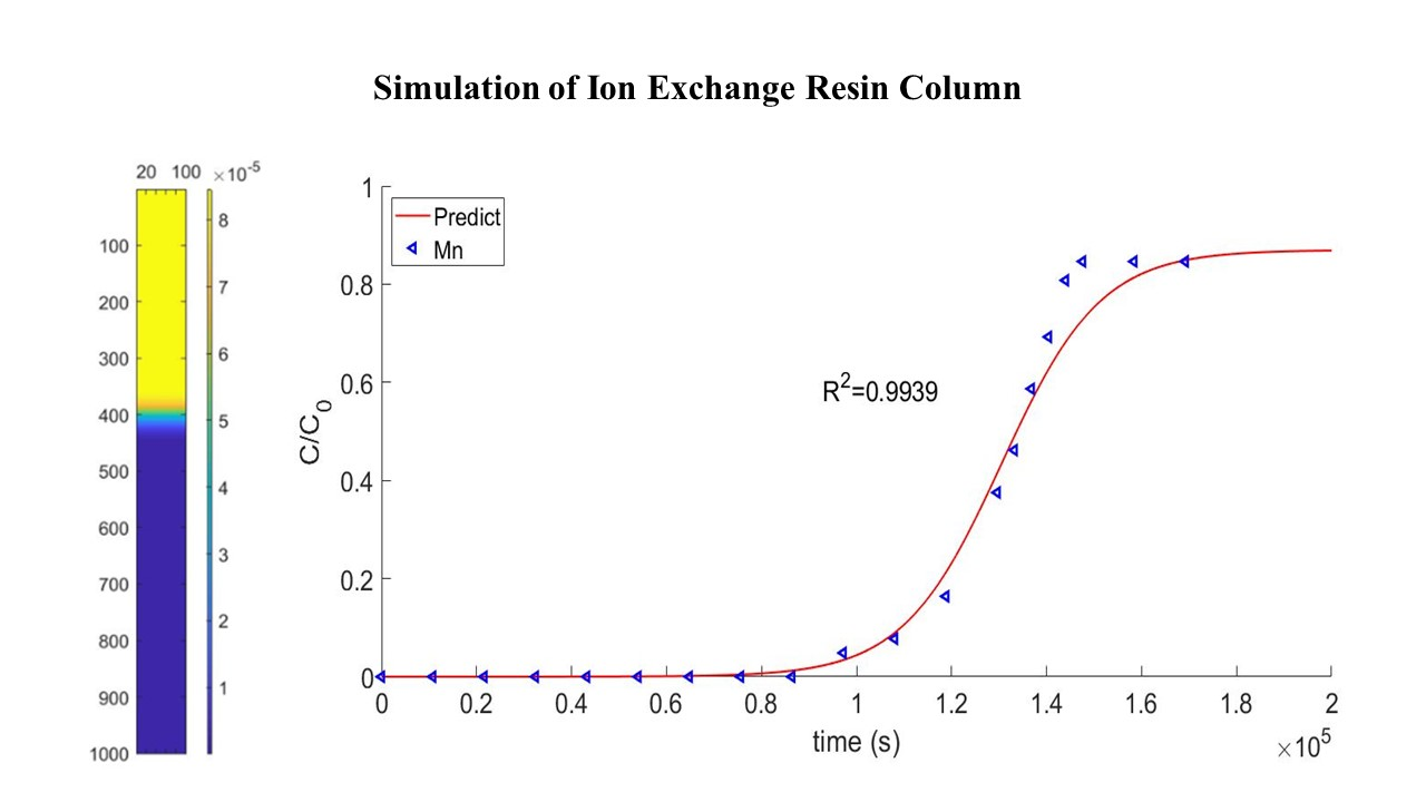
4.2. Analysis of Theoretical Results

Accuracy of the model was assessed by comparing the calculated values of effluent over time to the experimentally determined values for several different ions. Visualization of data is a unique aspect in this work, and convergence of the equation is essential to a successful calculation with this model. The equation could be adjusted at the same time to achieve the purpose of getting close to the actual situation. The predicted curves were obtained by using the last space point data from the matrix and conducting iterative calculations. Experimental data for Mn²⁺ were obtained using a real-time conductivity meter. It was assumed that when the value of C/C₀ reached 0.05, the resin was at the breakthrough point. In general, the model closely matched the experimental data for Mn²⁺, which is of particular significance because the Mn²⁺ ion is the main impurity in the coolant of a nuclear reactor. Thus, the main calculation target is based on the experimental condition of Mn²⁺. To further validate the model, calculated predictions were also compared to experimental data for Cl^-, and the results are shown in Figure 3.

Validation of the model requires a comparison between the calculated curve of the effluent concentration and the actual breakthrough curve. The comparison of the calculated model to the experimental Mn²⁺ test data is shown in Figure 4. The two groups of data had a good fitting degree and a consistent trend of change for their correlation coefficients, which were 0.9939 and 0.9893, respectively. Thus, it can be concluded that the model verified the test data. Breakthrough points were obtained, as shown in Figure 4. As a practical matter, the breakthrough point can be used to determine when the resin used in the first circuit of a nuclear reactor should be discarded.

The breakthrough point means the time point when the breakthrough curve shows an upwind trend. The breakthrough time of the three ions is compared in Table 2.

The comparative results between the experimental value and the calculated value meet our modeling requirements. When calculating different ions, the modification coefficient of the model is very close, indicating that the model is stable.

The advantage of a finite element method is the integrity of the solution, and thus the concentration changing processes are shown in Figure 5 and Figure 6. Previous articles just exhibited the concentration changing curve in the effluent. Figure 5 shows the different changing processes from inflow to outflow. Putting every concentration changing curve in the same picture can directly show the difference in different positions.

Figure 5 shows the concentration curves calculated every 100 space intervals in the column. Starting from the entrance, 11 curves of concentration over time were obtained by calculating every 100 spatial nodes. It is clear that the concentration changes with time at different spatial points. In particular, from the inlet to outlet of the column, the slope decreases because it is the same as the actual situation. Obviously, the ion exchange process, indeed, is fiercer because the local capacity of resin is lower in the lower part of column. In the essence of the algorithm, the iterative calculation gives the equation the ability to exhibit the changing process of the adsorption capacity.

To observe the concentration changing process of the column more intuitively, the data of the matrix is transformed to the colorful diagram shown in Figure 6. Using imagesc function in Matlab, the concentration data is expressed using different colors. With the colorbar function, the colorbar nearing the colormap figure shows the value changing process. Thus, there are six calculation results for the column transformation in every 2000 s.

As seen in Figure 6, through the built-in imagesc function in Matlab, the variation chart of concentration in the column is visualized with a very intuitive interval of 2000 s. Setting equal time interval points effectively shows the variation trend of the concentration in the column at different positions. In the Figure 6, the yellow part represents the “failure layer”, the blue part represents the “inactive layer”, and between them is the “working layer”. This mode of visualizing the data very intuitively shows that as ion exchange continues over time, the “working layer” moves down the column. Moreover, one can see an overall trend that effluent concentration decreases over time.

5. Conclusions

Ion exchange resins are crucial to the functioning and safety of modern water-cooled nuclear reactors because they remove metal ions that would otherwise corrode a reactor’s coolant system. However, to date there has not been a satisfactory mathematical model to predict the optimal operational lifetime of a resin bed. This work modeled resin ion exchange behavior using a system of PDEs based on the conservation of matter and then solved it using the method of finite differences. Using Matlab, the behavior of a resin bed can then be calculated via an iterative approach not merely over time, as in past studies, but over the spatial coordinate of the position of resin beads in the column. Theoretical results of this model proved to be in good agreement with experimental results using real ion exchange columns and Mn²⁺, which is the main contaminant found in reactor coolant water. Furthermore, simulation of the dynamic process is obtained, which clearly exhibits a concentration changing trend. The results show that this model has great potential to be used in nuclear engineering applications because a more efficient use of resin will not only cut costs but also reduce the quantity of toxic waste produced.

Author Contributions

Y.Z. for writing-original draft: and software; B.L. for data curation; R.P. for review&editing; Y.L. and P.Y. for supervision.

Funding

This research received no external funding.

Conflicts of Interest

The authors declare no conflicts of interest.

Abbreviations

$a_{i}$	Parameter of ion i
$b_{i}$	Parameter of ion i
$c_{g}$	Total equivalent concentration (keq/m3)
$c_{i}$	Concentration of ion i (kmol/m3)
C	Liquid phase concentration (mol/L)
C₀	Initial liquid phase concentration (mol/L)
dt	Time step (s)
d_p	Diameter of resin particle (m)
$D_{i}$	Individual diffusivity of ion i (m²/s)
$D$	Representative diffusivity (m²/s)
E	Back mixing coefficient (dimensionless)
F	Faraday’s constant
H	Height of column (m)
J	Ion flux (mol/m²·s)
t	Time (s)
q	Adsorption capacity (mg/g)
S	Cross-section area (m²)
u	Linear velocity (m/s)
U_L	Superficial velocity (m/s)
$ε$	Void fraction (dimensionless)
k	Representative mass transfer coefficient (m/s)
m	Number of co-ions
$n_{i}$	Relative valence
Р	Exponent
$q_{i}$	Loading of ion i (mol/g)
R	Gas law constant
T	Temperature
$u_{i}$	Variable for the numerical solution
$x_{i}$	Equivalent fraction of ion i in the solution
$y_{i}$	Equivalent fraction of ion i in the resin phase
$z_{i}$	Electrochemical valence (negative for anions)
$δ$	Nernst film thickness (m)
$ρ_{p}$	Resin particle density(kg/m³)
$ω_{i}$	$ω_{}$ of the counterions

Appendix A

Based on the conservation of matter, an infinitesimal distance from the ion exchange column was studied. Flux through the column (mol/m² s) was defined as consisting of the mainstream and back mixing:

J = u C - E \frac{\partial C}{\partial H}

(A1)

where J is the flux of the column, u is the velocity of flow, C is the concentration at height H, and E is the back-mixing coefficient.

According to the Taylor expansion:

f (x + Δ x) = f (x) + \frac{\partial}{\partial x} f (x) \cdot Δ x + \frac{1}{2!} \frac{\partial^{2}}{\partial x^{2}} f (x) \cdot Δ x^{2} + \dots

(A2)

Equation (A1) with the Taylor expansion deformation can be written as:

J_{H + d H} = (u C - E \frac{\partial C}{\partial H}) + \frac{\partial}{\partial H} (u C - E \frac{\partial C}{\partial H}) Δ H

(A3)

Because of the conservation of matter, one can assume that the inflow is equal to the effluent plus the accumulation in the solid and liquid phases. This gives:

ε S (J_{H} - J_{H + d H}) = ε S \frac{\partial C}{\partial H} d H + (1 - ε) S \frac{\partial q}{\partial t} d H

(A4)

where,

$ε S (J_{H} - J_{H + d H})$ is the inflow minus outflow in the interface
$ε S \frac{\partial C}{\partial H} d H$ is the change of ions in the microelement, and
$(1 - ε) S \frac{\partial q}{\partial t} d H$ is the ion change in the resin.

Combining Equations (1), (3), and (4) yields:

u \frac{\partial C}{\partial H} + \frac{\partial C}{\partial t} + (\frac{1 - ε}{ε}) \frac{\partial q}{\partial t} = E \frac{\partial^{2} C}{\partial H^{2}}

(A5)

Most prior studies on this subject were based on the one-dimensional convection equation, and the various groups made different choices when deciding the magnitude of the change in the rate of adsorption. Most of them also chose to omit the back-mixing term to simplify the calculation. This assumption is indeed suitable for lab scale experiments. Therefore, the righthand side of Equation (A4) is assumed to be negligibly small:

u \frac{\partial C}{\partial H} + \frac{\partial C}{\partial t} + (\frac{1 - ε}{ε}) \frac{\partial q}{\partial t} = 0

(A6)

According to previous literature [18], thin-film diffusion is governed by the concentration difference equation:

\frac{\partial q}{\partial t} = \frac{6}{d_{p}} J_{i}

(A7)

where

d_{p}

is the diameter of the resin particles, of which the average value is given in Table 1. By combining the above two equations, the one-dimensional convection equation in this special format can be solved using the finite difference method, and the concentration values at different time and space nodes can be calculated.

The following is the derivation process of J_i:

J_{i} = - D_{i} [\frac{\partial c_{i}}{\partial ξ} + z_{i} \frac{c_{i} F}{R T} \frac{\partial ϕ}{\partial ξ}]

(A8)

Because of the assumption that there is no net electric current, the following can be written:

\sum_{i = 1}^{n} z_{i} J_{i} = 0

(A9)

By both sides of Equation (A9) by

z_{i}

and taking the sum, the following can be derived:

\begin{array}{l} \sum_{j = 1}^{m} z_{i} J_{i} = - \sum_{i = 1}^{m} D_{i} z_{i} [\frac{d c_{i}}{d ξ} + z_{i} \frac{c_{i} F}{R T} \frac{d φ}{d ξ}] = 0 \\ \sum_{i = 1}^{m} D_{i} z_{i} \frac{d c_{i}}{d ξ} + \sum_{i = 1}^{m} D_{i} z_{i}^{2} \frac{c_{i} F}{R T} \frac{d φ}{d ξ} = 0 \end{array} \frac{d φ}{d ξ} = - \frac{R T}{F} \frac{\sum_{i = 1}^{m} z_{i} \frac{d c_{i}}{d ξ}}{\sum_{i = 1}^{m} z_{i}^{2} C_{i}}

(A10)

The total equivalent concentration

c_{g}

is introduced to give:

c_{g} = ω \sum_{i = 1}^{n} z_{i} C_{i}

(A11)

The mean value for the co-ion valence is introduced to yield:

z_{Y} = \frac{\sum_{i = 1}^{m} z_{i}^{2} c_{i}}{\sum_{i = 1}^{m} z_{i} J_{i}}

(A12)

Equations (A11) and (A12) are substituted into Equation (A10) which results in the following equation:

\frac{d φ}{d ξ} = - \frac{R T}{z_{Y} F} \frac{1}{c_{g}} \frac{d c_{g}}{d ξ}

(A13)

Equation (A13) is substituted into Equation (A8), and the following is obtained:

J_{i} = - D_{i} [\frac{{dc}_{i}}{d ξ} + n_{i} \frac{c_{i}}{R T} \frac{d c_{g}}{d ξ}]

(A14)

where

n_{i} = - \frac{z_{i}}{z_{Y}}

.

ξ

is derived from both sides of Equation (A14) as follows:

\begin{array}{l} 0 = - D_{i} [\frac{d^{2} c_{i}}{d ξ^{2}} + n_{i} d (\frac{c_{i}}{c_{g}} \frac{d c_{g}}{d ξ}) / d ξ] \\ \frac{d^{2} c_{i}}{d ξ^{2}} + n_{i} (\frac{d^{2} c_{g}}{d ξ^{2}} \frac{c_{i}}{c_{g}} + \frac{{dc}_{g}}{d ξ} \frac{d (\frac{c_{i}}{c_{g}})}{d ξ}) = 0 \end{array} \frac{d^{2} c_{i}}{d ξ^{2}} + \frac{n_{i}}{c_{g}} \frac{{dc}_{i}}{d ξ} \frac{{dc}_{g}}{d ξ} + n_{i} \frac{c_{i}}{c_{g}} (\frac{d^{2} c_{g}}{d ξ^{2}} - \frac{1}{c_{g}} {(\frac{{dc}_{g}}{d ξ})}^{2}) = 0

(A15)

Both sides of Equation (A15) are summed to give:

\sum_{i = 1}^{n} \frac{d^{2} c_{i}}{d ξ^{2}} + \frac{1}{c_{g}} \frac{{dc}_{g}}{d ξ} \sum_{i = 1}^{n} n_{i} \frac{{dc}_{i}}{d ξ} + \frac{1}{c_{g}} \frac{d^{2} c_{g}}{d ξ^{2}} \sum_{i = 1}^{n} n_{i} c_{i} - \frac{1}{c_{g}^{2}} {(\frac{{dc}_{g}}{d ξ})}^{2} \sum_{i = 1}^{n} n_{i} c_{i} = 0

(A16)

According to Equation (A11):

\frac{{dc}_{g}}{d ξ} = ω \sum_{i = 1}^{n} z_{i} \frac{{dc}_{i}}{d ξ}

This is substituted into Equation (A16) to give:

\frac{d^{2} c_{g}}{d ξ^{2}} = 0

(A17)

According to the chain rule, the following can be written:

\begin{array}{l} \frac{{dc}_{i}}{d ξ} = m_{g} \frac{{dc}_{i}}{d c_{g}} \\ \frac{d^{2} c_{i}}{d ξ^{2}} = m_{g}^{2} \frac{d^{2} c_{i}}{d c_{g}^{2}} \end{array} m_{g} = \frac{{dc}_{g}}{d ξ}

(A18)

Equations (A17) and (A18) are substituted into Equation (A15), and the following is obtained:

\frac{d^{2} c_{i}}{d c_{g}^{2}} + \frac{n_{i}}{c_{g}} \frac{{dc}_{i}}{d c_{g}} - \frac{n_{i} c_{i}}{c_{g}^{2}} = 0

(A19)

Equation (A19) is a second-order homogeneous linear differential equation (Euler equation). According to the relationship between

c_{g}

and t:

\begin{array}{l} c_{g} = e^{t} \\ t = \ln (c_{g}) \\ \frac{d^{2} c_{i}}{d c_{g}^{2}} = \frac{1}{c_{g}^{2}} (\frac{d^{2} c_{i}}{d t^{2}} - \frac{{dc}_{i}}{d t}) \\ \frac{{dc}_{i}}{d c_{g}} = \frac{{dc}_{i}}{d t} \frac{1}{c_{g}} \end{array}

A constant coefficient linear differential equation is obtained:

\frac{d^{2} c_{i}}{d t^{2}} + (n_{i} - 1) \frac{{dc}_{i}}{d t} - n_{i} c_{i} = 0 c_{i} = a_{i}^{'} c_{g} + b_{i}^{'} c_{g}^{- P}

(A20)

where

P {= n}_{i}

z_{i} c_{i} = a_{i} c_{g} + b_{i} c_{g}^{- P}

(A21)

The following is determined by boundary conditions:

a_{i} = \frac{1}{c_{g}} (z_{i} c_{i}^{b} - b_{i} {(c_{g}^{b})}^{- P}) b_{i} = \frac{\frac{z_{i} c_{i}^{s}}{c_{g}^{s}} - \frac{z_{i} c_{i}^{b}}{c_{g}^{b}}}{{(c_{g}^{s})}^{- P - 1} - {(c_{g}^{b})}^{- P - 1}} = ω \frac{x_{i}^{s} - x_{i}^{b}}{{(c_{g}^{s})}^{- P - 1} - {(c_{g}^{b})}^{- P - 1}}

(A22)

For a_i, the following can be written for b_i:

\sum_{i = 1}^{n} a_{i} = ω; \sum_{i = 1}^{n} b_{i} = 0

(A23)

The derivative of Equation (A22) gives:

z_{i} \frac{{dc}_{i}}{d ξ} = a_{i} \frac{{dc}_{g}}{d ξ} + b_{i} \frac{{dc}_{_{g}}^{- P}}{d ξ} = a_{i} \frac{{dc}_{g}}{d ξ} - b_{i} P c_{_{g}}^{- P - 1} \frac{{dc}_{g}}{d ξ}

The above equation is substituted into Equation (A14) to give:

J_{i} = - \frac{D_{i}}{z_{i}} \frac{{dc}_{g}}{d ξ} [(a_{i} - b_{i} P c_{_{g}}^{- P - 1}) + n_{i} (a_{i} + b_{i} P c_{_{g}}^{- P - 1})]

(A24)

with

P {= n}_{i}

:

J_{i} = - \frac{D_{i}}{z_{i}} \frac{{dc}_{g}}{d ξ} (1 + n_{i}) a_{i}

(A25)

Both sides are multiplied by

z_{i}

, and the equation is combined with Equation (A10) to give:

\sum_{i = 1}^{n} D_{i} a_{i} = 0

(A26)

With the definitions of

a_{i}

and

b_{i}

, the following can be written:

\sum_{i = 1}^{n} D_{i} ω x_{i}^{b} = {(c_{g}^{b})}^{- P - 1} \times \sum_{i = 1}^{n} D_{i} ω \frac{x_{i}^{s} - x_{i}^{b}}{{(c_{g}^{s})}^{- P - 1} - {(c_{g}^{b})}^{- P - 1}}

(A27)

After algebraic transformation, the following is obtained:

c_{g}^{s} = {(\frac{\sum_{i = 1}^{n} D_{i} x_{i}^{b}}{\sum_{i = 1}^{n} D_{i} x_{i}^{s}})}^{\frac{1}{P + 1}} c_{g}^{b}

(A28)

Derivatives of Equation (A26) on both sides of

ξ

give:

\begin{array}{l} \int_{0}^{δ} J_{i} d ξ = - \frac{D_{i}}{z_{i}} (1 + n_{i}) a_{i} \int_{0}^{δ} \frac{{dc}_{g}}{d ξ} d ξ \\ J_{i} δ = - \frac{D_{i}}{z_{i}} (1 + n_{i}) a_{i} c_{g} |_{0}^{δ} \end{array}

The boundary conditions are as follows:

\begin{array}{l} ξ = 0, c_{g} = c_{g}^{s} \\ ξ = δ, c_{g} = c_{g}^{b} \end{array}

Thus, the following is obtained:

J_{i} = \frac{D_{i} a_{i}}{z_{i} δ} (1 + n_{i}) (c_{g}^{s} - c_{g}^{b})

(A29)

Kataoka [32] mentioned the following:

P = \frac{n_{A} D_{A} - n_{B} D_{B}}{D_{A} - D_{B}}

(A30)

Both sides of Equation (A24) are multiplied by

z_{i}

with the assumption that there is no net electric current and that

\frac{{dc}_{g}}{d ξ}

is not zero, and thus the following is obtained:

(\sum_{i = 1}^{n} D_{i} a_{i} + \sum_{i = 1}^{n} n_{i} D_{i} a_{i}) + (\sum_{i = 1}^{n} n_{i} D_{i} b_{i} - P \sum_{i = 1}^{n} D_{i} b_{i}) c_{g}^{- P - 1} = 0

(A31)

Equation (A31) is valid at any point in the liquid film. The value of

c_{g}

is independent of the position, and thus the expressions in parentheses are all zero.

\sum_{i = 1}^{n} (n_{i} + 1) D_{i} a_{i} = 0

(A32)

For the total equivalent concentration, the following can be written:

c_{_{g}}^{s} = {[\frac{\sum_{i = 1}^{n} (n_{i} + 1) D_{i} x_{_{i}}^{b}}{\sum_{i = 1}^{n} (n_{i} + 1) D_{i} x_{_{i}}^{s}}]}^{\frac{1}{P + 1}} c_{_{g}}^{b}

(A33)

x_{i} = \frac{ω z_{i} c_{i}}{c_{g}} \sum_{i = 1}^{n} n_{i} D_{i} b_{i} - P \sum_{i = 1}^{n} D_{i} b_{i} = 0

(A34)

When this is combined with the definition of

b_{i}

, the following is obtained:

P = \frac{\sum_{i = 1}^{n} n_{i} D_{i} (x_{_{i}}^{s} - x_{_{i}}^{b})}{\sum_{i = 1}^{n} D_{i} (x_{_{i}}^{s} - x_{_{i}}^{b})}

(A35)

With Equations (A22) and (A26), we obtain the final target function:

J_{i} = \frac{D_{i} a_{i}}{z_{i} δ} (n_{i} + 1) (c_{g}^{s} - c_{g}^{b}) - \frac{D_{i} b_{i}}{z_{i} δ} \frac{n_{i} - P}{P} ({(c_{g}^{s})}^{- P} - {(c_{g}^{b})}^{- P})

(A36)

J_{i} = \frac{D_{i}}{z_{i}} [(1 - \frac{n_{i}}{P}) (c_{i}^{s} - c_{i}^{b}) + \frac{a_{i} n_{i}}{z_{i}} (c_{g}^{s} - c_{g}^{b}) (1 + \frac{1}{P})]

(A37)

This PDE describing the change of concentration in the column, as obtained above using material balance and Taylor’s expansion formula, is the theoretical basis and main formula in this work.

To solve this PDE using the finite difference method, upwind difference scheme of the PDE follows:

\frac{6 J_{i}}{d_{p}} \frac{1 - ε}{ε} + \frac{c_{i} (h_{j}, t_{n + 1}) - c_{i} (h_{j}, t_{n})}{τ} + U_{L} \frac{c_{i} (h_{j}, t_{n}) - c_{i} (h_{j - 1}, t_{n})}{h} = 0

(A38)

This upwind difference scheme constitutes one solution to this set of PDE. It has two forms, one contains the forward difference, and the other contains the backward difference. Obviously, U_L is greater than zero, and thus it is shown as Equation (38).

References

Smith, R.P.; Woodburn, E.T. Prediction of Multicomponent Ion Exchange Equilibria for the Ternary System SO-NO-Cl from Data of Binary Systems. AIChE J. 1978, 24, 577–587. [Google Scholar] [CrossRef]
Haub, C.E.; Foutch, G.L. Mixed-bed ion exchange at concentrations approaching the dissociation of water. 2. Column model applications. Ind. Eng. Chem. Res. 1986, 25, 381–385. [Google Scholar] [CrossRef]
Zecchini, E.J.; Foutch, G.L.; Yoon, T. Multi-Component Mixed-Bed Ion Exchange Modeling in Aminated Waters. In Ion Exchange. Advances; Springer: Dordrecht, The Netherlands, 1992. [Google Scholar]
Yang, J.E.; Skogley, E.O. Diffusion Kinetics of Multinutrient Accumulation by Mixed-Bed Ion-Exchange Resin. Soil Sci. Soc. Am. J. 1992, 56, 408. [Google Scholar] [CrossRef]
Hall, K.R.; Eagleton, L.C.; Acrivos, A.; Vermeulen, T. Pore- and Solid-Diffusion Kinetics in Fixed-Bed Adsorption under Constant-Pattern Conditions. Ind. Eng. Chem. Fundam. 1966, 5, 587–594. [Google Scholar] [CrossRef]
Dwivedi, P.N.; Upadhyay, S.N. Particle-Fluid Mass Transfer in Fixed and Fluidized Beds. Ind. Eng. Chem. Process Des. Dev. 1977, 16, 157–165. [Google Scholar] [CrossRef]
Shams, K. Sorption dynamics of a fixed-bed system of thin-film-coated monodisperse spherical particles/hollow spheres. Chem. Eng. Sci. 2001, 56, 5383–5390. [Google Scholar] [CrossRef]
Chowdiah, V.N.; Foutch, G.L.; Lee, G.C. Binary Liquid-Phase Mass Transport in Mixed-Bed Ion Exchange at Low Solute Concentration. Ind. Eng. Chem. Res. 2003, 42, 1485–1494. [Google Scholar] [CrossRef]
Lim, A.P.; Aris, A.Z. Continuous fixed-bed column study and adsorption modeling: Removal of cadmium (II) and lead (II) ions in aqueous solution by dead calcareous skeletons. Biochem. Eng. J. 2014, 87, 50–61. [Google Scholar] [CrossRef]
Yu, Q.; Wang, N.H.L. Computer simulations of the dynamics of multicomponent ion exchange and adsorption in fixed beds—Gradient-directed moving finite element method. Comput. Chem. Eng. 1989, 13, 915–926. [Google Scholar] [CrossRef]
Carta, G.; Cincotti, A.; Cao, G. Film Model Approximation for Particle-Diffusion-Controlled Binary Ion Exchange. Sep. Sci. Technol. 1999, 34, 1–16. [Google Scholar] [CrossRef]
Spalding, G.E. Predictive Theory of Coion Transport Accompanying Particle-Diffusion-Controlled Ion Exchange. J. Chem. Phys. 1971, 55, 4991–4995. [Google Scholar] [CrossRef]
Rahmant, K.; Streat, M. Mass transfer in liquid fluidized beds of ion exchange particles. Chem. Eng. Sci. 1981, 36, 293–300. [Google Scholar] [CrossRef]
Zecchini, E.J.; Foutch, G.L. Mixed-bed ion-exchange modeling with amine form cation resins. Ind. Eng. Chem. Res. 1991, 30, 1886–1892. [Google Scholar] [CrossRef]
Janvion, P.; Motellier, S.; Pitsch, H. Ion-exchange mechanisms of some transition metals on a mixed-bed resin with a complexing eluent. J. Chromatogr. A 1995, 715, 105–115. [Google Scholar] [CrossRef]
Fenn, M.E.; Poth, M.A.; Arbaugh, M.J. A throughfall Collection Method Using Mixed Bed Ion Exchange Resin Columns. Sci. World J. 2002, 2, 122–130. [Google Scholar] [CrossRef]
Korak, J.A.; Huggins, R.; Arias-Paic, M. Regeneration of pilot-scale ion exchange columns for hexavalent chromium removal. Water Res. 2017, 118, 141–151. [Google Scholar] [CrossRef]
Franzreb, M.; Hoell, W.H.; Eberle, S.H. Liquid-Phase Mass Transfer in Multicomponent Ion Exchange. 2. Systems with Irreversible Chemical Reactions in the Film. Ind. Eng. Chem. Res. 1995, 34, 2670–2675. [Google Scholar] [CrossRef]
FREY, D.D. Prediction of liquid-phase mass-transfer coefficients in multicomponent ion exchange: Comparison of matrix, film-model, and effective-diffusivity methods. Chem. Eng. Commun. 1986, 47, 273–293. [Google Scholar] [CrossRef]
Chatterjee, A.; Schiewer, S. Multi-resistance kinetic models for biosorption of Cd by raw and immobilized citrus peels in batch and packed-bed columns. Chem. Eng. J. 2014, 244, 105–116. [Google Scholar] [CrossRef]
Rosen, J.B. Kinetics of a Fixed Bed System for Solid Diffusion into Spherical Particles. J. Chem. Phys. 1952, 20, 387–394. [Google Scholar] [CrossRef]
Jia, Yi.; Foutch, G.L. True multi-component mixed-bed ion-exchange modeling. React. Funct. Polym. 2004, 60, 121–135. [Google Scholar] [CrossRef]
Ebrahimi, S.; Roberts, D.J. Mathematical modelling and reactor design for multi-cycle bioregeneration of nitrate exhausted ion exchange resin. Water Res. 2016, 88, 766–776. [Google Scholar] [CrossRef] [PubMed]
Xiu, G.H.; Li, P. Prediction of breakthrough curves for adsorption of lead(II) on activated carbon fibers in a fixed bed. Carbon 2000, 38, 975–981. [Google Scholar] [CrossRef]
Wu, J.; Jia, L.; Wu, L.; Long, C.; Deng, W.; Zhang, Q. Prediction of the breakthrough curves of VOC isothermal adsorption on hypercrosslinked polymeric adsorbents in a fixed bed. RSC Adv. 2016, 6, 28986–28993. [Google Scholar] [CrossRef]
Yoshida, H.; Kataoka, T. Intraparticle ion-exchange mass transfer in a ternary system. Ind. Eng. Chem. Res. 1987, 26, 1179–1184. [Google Scholar] [CrossRef]
Chern, J.M.; Chien, Y.W. Adsorption of nitrophenol onto activated carbon: Isotherms and breakthrough curves. Water Res. 2002, 36, 647–655. [Google Scholar] [CrossRef]
Faizal, A.M.; Kutty, S.R.M.; Ezechi, E.H. Modelling of Adams-Bohart and Yoon-Nelson on the Removal of Oil from Water Using Microwave Incinerated Rice Husk Ash (MIRHA). Appl. Mech. Mater. 2014, 625, 788–791. [Google Scholar] [CrossRef]
Bohart, G.S.; Adams, E.Q. Some aspects of the behavior of charcoal with respect to chlorine. J. Am. Chem. Soc. 1920, 189, 669. [Google Scholar]
Aksu, Z.; Gönen, F. Biosorption of phenol by immobilized activated sludge in a continuous packed bed: Prediction of breakthrough curves. Process Biochem. 2004, 39, 599–613. [Google Scholar] [CrossRef]
Kataoka, T.; Sato, N.; Ueyama, K. Effective liquid phase diffusivity in ion exchange. Chem. Eng. Jpn. 1968, 1, 38–42. [Google Scholar] [CrossRef]
Kataoka, T.; Yoshida, H.; Uemura, T. Liquid-side ion exchange mass transfer in a ternary system. AIChE J. 1987, 33, 202–210. [Google Scholar] [CrossRef]
Lin, X.; Li, R.; Wen, Q.; Wu, J.; Fan, J.; Jin, X.; Qian, W.; Liu, D.; Chen, X.; Chen, Y.; et al. Experimental and modeling studies on the sorption breakthrough behaviors of butanol from aqueous solution in a fixed-bed of KA-I resin. Biotechnol. Bioprocess Eng. 2013, 18, 223–233. [Google Scholar] [CrossRef]
Mabrouk, A.; Lagneau, V.; De Dieuleveult, C.; Bachet, M.; Schneider, H.; Coquelet, C. Experiments and Modeling of Ion Exchange Resins for Nuclear Power Plants. Int. J. Eng. Appl. Sci. 2012, 6, 130–134. [Google Scholar]
Yang, J.; Renken, A. Intensification of mass transfer in liquid fluidized beds with inert particles. Chem. Eng. Process. Process Intensif. 1998, 37, 537–544. [Google Scholar] [CrossRef] [Green Version]
Murillo, R.; Garcıa, T.; Aylón, E.; Callén, M.S.; Navarro, M.V.; López, J.M.; Mastral, A.M. Adsorption of phenanthrene on activated carbons: Breakthrough curve modeling. Carbon 2004, 42, 2009–2017. [Google Scholar] [CrossRef]
Pan, B.C.; Meng, F.W.; Chen, X.Q.; Pan, B.J.; Li, X.T.; Zhang, W.M.; Zhang, X.; Chen, J.L.; Zhang, Q.X.; Sun, Y. Application of an effective method in predicting breakthrough curves of fixed-bed adsorption onto resin adsorbent. J. Hazard. Mater. 2005, 124, 74–80. [Google Scholar] [CrossRef] [PubMed]
Franzreb, M.; Höll, W.H.; Sontheimer, H. Liquid-phase mass transfer in multi-component ion exchange I. Systems without chemical reactions in the film. React. Polym. 1993, 21, 117–133. [Google Scholar] [CrossRef]
Bachet, M.; Jauberty, L.; De Windt, L.; Tevissen, E.; De Dieuleveult, C.; Schneider, H. Comparison of Mass Transfer Coefficient Approach and Nernst–Planck Formulation in the Reactive Transport Modeling of Co, Ni, and Ag Removal by Mixed-Bed Ion-Exchange Resins. Ind. Eng. Chem. Res. 2014, 53, 11096–11106. [Google Scholar] [CrossRef]
Tedesco, M.; Hamelers, H.V.M.; Biesheuvel, P.M. Nernst-Planck transport theory for (reverse) electrodialysis: I. Effect of co-ion transport through the membranes. J. Membr. Sci. 2016, 510, 370–381. [Google Scholar] [CrossRef]

Figure 1. Test flowchart.

Figure 2. Curve with different time step (dt) computations.

Figure 3. Breakthrough curve of Cl⁻.

Figure 4. Breakthrough curve of Mn²⁺.

Figure 5. Calculation of different position concentration curves.

Figure 6. Modeling of concentration in the column changing process.

Table 1. Information of ZhengGuang resin.

Name of Index	Cationic Resin	Anionic Resin
Classification form	gel-type	gel-type
functional group	-SO³	-N(CH³)³
Ion form	H⁺	OH^-
Volume full exchange capacity (mmol/mL)	≥1.80	≥1.10
Ratio of anion resin to anion resin (V/V)	1.0	2.0
particle size range mm	0.40–1.20	0.40–1.20
Wet apparent density (g/mL)	0.68–0.78	0.68–0.78
Maximum operating temperature (°C)	60.0	60.0
Ratio of H⁺	≥99.9%	-
Ratio of OH⁻	-	≥95.0%

Table 2. Information on the breakthrough point.

Target Ion (10⁴ s)	Experimental Value	Calculate Value
K⁺	16.21	11.14
Cl⁻	6.15	6.16
Mn²⁺	8.64	8.66

© 2019 by the authors. Licensee MDPI, Basel, Switzerland. This article is an open access article distributed under the terms and conditions of the Creative Commons Attribution (CC BY) license (http://creativecommons.org/licenses/by/4.0/).

Share and Cite

MDPI and ACS Style

Zhu, Y.; Liu, B.; Peng, R.; Luo, Y.; Yu, P. Simulation of Ion Exchange Resin with Finite Difference Methods. Processes 2019, 7, 675. https://doi.org/10.3390/pr7100675

AMA Style

Zhu Y, Liu B, Peng R, Luo Y, Yu P. Simulation of Ion Exchange Resin with Finite Difference Methods. Processes. 2019; 7(10):675. https://doi.org/10.3390/pr7100675

Chicago/Turabian Style

Zhu, Yawen, Bobo Liu, Ruichao Peng, Yunbai Luo, and Ping Yu. 2019. "Simulation of Ion Exchange Resin with Finite Difference Methods" Processes 7, no. 10: 675. https://doi.org/10.3390/pr7100675

Note that from the first issue of 2016, this journal uses article numbers instead of page numbers. See further details here.

Article Menu

Simulation of Ion Exchange Resin with Finite Difference Methods

Abstract

1. Introduction

2. Modeling

2.1. Modeling Assumptions

2.2. Equations

2.3. Initial Condition

2.4. Numerical Method

3. Experiment

4. Results and Discussion

4.1. Convergence of the Model

4.2. Analysis of Theoretical Results

5. Conclusions

Author Contributions

Funding

Conflicts of Interest

Abbreviations

Appendix A

References

Share and Cite

Article Metrics

Article Access Statistics

Further Information

Guidelines

MDPI Initiatives

Follow MDPI