Fine-Tuning Meta-Heuristic Algorithm for Global Optimization

Abstract

This paper proposes a novel meta-heuristic optimization algorithm called the fine-tuning meta-heuristic algorithm (FTMA) for solving global optimization problems. In this algorithm, the solutions are fine-tuned using the fundamental steps in meta-heuristic optimization, namely, exploration, exploitation, and randomization, in such a way that if one step improves the solution, then it is unnecessary to execute the remaining steps. The performance of the proposed FTMA has been compared with that of five other optimization algorithms over ten benchmark test functions. Nine of them are well-known and already exist in the literature, while the tenth one is proposed by the authors and introduced in this article. One test trial was shown to check the performance of each algorithm, and the other test for 30 trials to measure the statistical results of the performance of the proposed algorithm against the others. Results confirm that the proposed FTMA global optimization algorithm has a competing performance in comparison with its counterparts in terms of speed and evading the local minima.

1. Introduction

Meta-heuristic optimization describes a broad spectrum of optimization algorithms that need only the relevant objective function along with key specifications, such as variable boundaries and parameter values. These algorithms can locate the near-optimum, or perhaps the optimum values of that objective function. In general, meta-heuristic algorithms simulate the physical, biological, or even chemical processes that happen in nature. Of the meta-heuristic optimization algorithms, the following are the most widely used:

• Genetic algorithms (GAs) [1], which simulate Darwin’s theory of evolution;
• Simulated annealing (SA) [2], which emerged from the thermodynamic argument;
• Ant colony optimization (ACO) algorithms [3], which mimic the behavior of an ant colony foraging for food;
• Particle swarm optimization (PSO) algorithms [4], which simulates the behavior of a flock of birds;
• Artificial bee colony (ABC) algorithms [5], which mimic the behavior of the honeybee colony; and
• Differential evolution algorithms (DEAs) [6], for solving global optimization problems.

Xing and Gao collected more than 130 state-of-the-art optimization algorithms in their book [7], and these swarm-based optimizations are applied in different applications and study cases [8,9,10,11,12,13,14]. Some algorithms start from a single point, such as SA, but the majority begin from a population of initial solutions (agents) like GAs, PSO, and DEAs, most of which is referred to as “swarm intelligence” in their mimicry of animal behaviors [15]. In these algorithms, every agent shares its information with other agents through a system of simple operations. This information sharing results in improvements to the algorithm performance and helps find the optimum or near-optimum solution(s) more quickly [3].

In any meta-heuristic optimization algorithm, there are three significant types of information exchange between a particular agent with other agents in the population. The first is called exploitation, which is a local search for the latest, and the best solution found so far. The second is called exploration, which is a global search using another agent existing in the problem space [16]. The third is called randomization, which is rarely used in some algorithms or may not be used at all. This last procedure is similar to exploration, but instead of an existing agent, a randomly-generated agent is used. For instance, ABC algorithms use randomization for the scout agent; therefore, it often succeeds in evading many local minima. Many algorithms begin with exploration and gradually shift to exploitation after several generations to avoid falling into local optimum values. Meta-heuristic algorithms then maintain trade between exploration and exploitation [17]. However, the different types demonstrate variations in how they perform this trade; by using this trade, these algorithms may get close to near-optimum or even optimum solutions.

All agents compete with themselves to stay alive inside the population. Every agent that improves its performance replaces any agent that did not promote itself. Therefore, in the fourth stage (i.e., selection) a variable selection method, such as greedy selection or roulette wheel, is used to choose the best agent to replace the worst one [1]. Meta-heuristic algorithms may find near-optimum solutions for some objective functions, but it may fall into local minima for other ones. This fact will be apparent in the results of this article. To date, an optimization algorithm that offers a superior convergence time and avoids local minima for objective functions has yet to be developed. Therefore, the area is open to improving the existing meta-heuristic algorithms or inventing new ones to fulfill these requirements [18].

In this article, a novel algorithm called the fine-tuning meta-heuristic algorithm (FTMA) is presented. It utilizes information sharing among the population agents in such a way that it finds the global optimum solution faster without falling into local ones; this is accomplished by performing the necessary optimization procedures sequentially. In the next section, the proposed algorithm is described in detail. Then, five well-known optimization algorithms are presented to compete with FTMA over a ten-function benchmark. The results and discussion are shown in the final section, along with the conclusions.

2. Literature Review

In the scope of the recent trends in nature-based meta-heuristic optimization algorithms, since the genetic algorithms [1] and simulated annealing [2] has been presented, the race begins in inventing many algorithms thanks to the rapid advances in computer speed and efficiency, especially in the new millennia. From these algorithms, we mention the firefly algorithm (FA) [19], cuckoo search (CS) [20], bat algorithm (BA) [21], flower pollination algorithm (FPA) [22], and many others mentioned in [23].

Many optimization algorithms were invented over the past five years. Some of them are new, and the others are modifications and enhancements to the already-existing ones. One of the recent and widely-used algorithms is grey wolf optimization (GWO) [24]; it is inspired by the grey wolves and their hunting behaviors in nature. Four types of leadership hierarchy of the grey wolves as well as three steps of prey hunting strategies are implemented. Mirjalili continued to invent other algorithms. The same authors presented moth–flame optimization (MFO) [25]. This algorithm mimics the navigation method of moths in nature which is called “traverse orientation”. The main path which the moths travel along is towards the Moon. However, they may fall into a useless spiral path around artificial lights if they encounter these in their way. Ant lion optimizer (ALO) has been proposed in [26], which simulated the hunting mechanism of antlions in nature. Five main steps of hunting are implemented in this algorithm. Moreover, the same authors of [24] proposed a novel population-based optimization algorithm, namely, the sine–cosine algorithm (SCA) [27], it fluctuates the solution agents towards, or outwards, the best solution using a model based on sine and cosine functions. It uses random and adaptive parameters to emphasize the search steps like exploration and exploitation. Another proposed algorithm in the literature is the whale optimization algorithm (WOA) [28]. This algorithm mimics the social behavior of humpback whales, using a hunting strategy called bubble-net, as well as three operators to simulate this hunting strategy. All these algorithms mentioned above are developed, enhanced, and modified through the years, hopefully to make them suitable for every real problem which needs solving. However, no-free-lunch theorems state that there is no single universal optimization method that can deal with every realistic problem [18].

3. Fine Tuning Meta-Heuristic Algorithm (FTMA)

The FTMA is a meta-heuristic optimization algorithm used to search for optimum solutions for simple and/or complex objective functions. The fundamental feature of FTMA is the fine-tuning meta-heuristic method used when searching for the optimum.

FTMA performs the fundamental procedures of solution update, which are exploration, exploitation, randomization, and selection in sequential order. In FTMA, the first procedure of exploration is undertaken concerning an arbitrarily-selected solution in the solution space. If the solution is not improved according to the probability, the second procedure of exploitation is performed concerning the best global solution found so far. Again, if the solution is not enhanced according to probability, then the third procedure of randomization is performed concerning a random solution generated in the solution space. The fourth procedure of selection is performed by comparing the new solution and the old one and choosing the best according to the objective function. The FTMA procedure steps are:

1) Initialization: FTMA begins with initialization. Its equation is shown below:

$$x_i^0\left(k\right)=lb\left(k\right)+rand\times \left(ub\left(k\right)-lb\left(k\right)\right);k=1.2.\dots d;i=1,2,\dots ,N.$$

(1)

At this point in the process, all the solutions $x_i^t$ are initialized randomly at the iteration counter $t=0$ according to the lower bound $lb$ and the upper bound $ub$ for each solution space index $k$ inside the solution space dimension $d$. A random number $rand$, its value is between 0 and 1, is used to place the solution value randomly somewhere between the lower and upper bounds. The space dimension, along with the number of solutions $N$ must be specified prior to the process. Then, the fitness $f_{xi}^0$ is evaluated for each solution $x_i^0$ using the objective function. The values of the best objective fitness $f_b^0$ and its associated best solution $x_b^0$ are initially obtained from the fitness and solutions vectors, respectively. Additionally, the probabilities of exploitation and randomization, $p,$ and $r,$ respectively, are initialized.

After incrementing the iteration counter inside of the generation iteration loop, the four steps in each iteration are performed in the FTMA core, as follows:

2) Exploration: The general formula of this step is as follows:

$$y\left(k\right)=x_i^t\left(k\right)+rand\times \left(x_j^t\left(k\right)-x_i^t\left(k\right)\right).$$

(2)

In this step, every solution $x_i^t$ is moved with respect to another existing solution vector$x_j^t$, where $j\ne i$. The value of the objective function for the temporary solution $y$ is then evaluated as a temporary fitness $g$.

3) Exploitation: Its equation is presented as follows:

$$ifg>f_{xi}^t\&\&p>rand,y\left(k\right)=x_i^t\left(k\right)+rand\times \left(x_b^t\left(k\right)-x_i^t\left(k\right)\right).$$

(3)

If the fitness $g$ is not improved compared with $f_{xi}^t$ and the probability of exploitation $p$ is greater than a random number $rand$; then the exploitation step will be initiated. In this step, the temporary solution vector $y$ is calculated by moving the solution $x_i^t$ with respect to the best global solution, $x_b^t$. The value of the objective function for the temporary solution $y$ is re-evaluated and stored in the temporary fitness $g$.

4) Randomization: The formula of this step is as follows:

$$ifg>f_{xi}^t\&\&r>rand,y\left(k\right)=x_i^t\left(k\right)+rand\times \left(lb\left(k\right)+rand\times \left(ub\left(k\right)-lb\left(k\right)\right)-x_i^t\left(k\right)\right).$$

(4)

If the fitness $g$ is not improved again in comparison with $f_{xi}^t$ and the probability of randomization $r$ is higher than a random number $rand$, then the randomization step will be initiated. In this step, the solution $x_i^t$ moves with respect to a randomly-generated solution. The value of the objective function for the temporary solution $y$ is again re-evaluated and then stored in the temporary fitness $g$.

5) Selection: The final step of the FTMA iteration process is the selection step, which is summarized as:

$$ifg<f_{xi}^t,x_i^{t+1}=y;f_{xi}^{t+1}=g,$$

(5)

$$ifg<f_b^t,x_b^{t+1}=y;f_b^{t+1}=g.$$

(6)

6) Stopping Condition: The search ends if the global fitness value $f_b^{t+1}$ reaches zero or below a specified tolerance value $\epsilon$, or if the iteration counter $t$ reaches its previously-specified maximum value $R$. The pseudocode of FTMA is summarized as in Algorithm 1 below.

4. Methodology

To check the validity of the proposed FTMA, it should be tested with different well-known optimization algorithms that were used widely in the literature. Five algorithms are chosen, although there are many.

4.1. Well-Known Optimization Algorithms

(1)

Genetic algorithm (decimal form) (DGA): This is similar to a conventional GAs with the exception that the chromosomes are not converted to binary digits. It has the same steps as GAs, selection, crossover, and mutation. Here, the crossover or mutation procedures are performed upon the decimal digits as they are performed upon the bits in a binary GA. The entire procedure of the DGA is taken from [29].

(2)

Genetic algorithm (real form) (RGA): In this algorithm, the vectors are used in optimization as real values, without converting them to integers or binary numbers. As a binary GA, it performs the same procedures. The complete steps of DGA are taken from [30].

(3)

Particle swarm optimization (PSO) with optimizer: The success of this famous algorithm is down to its simplicity. It uses the velocity vector to update every solution, using the best solution of the vector along with the best global solution found so far. The core formula of PSO is taken from [4].

(4)

Differential evolution algorithm (DEAs): This algorithm chooses two (possibly three) solutions other than the current solution and searches stochastically, using selected constants to update the current solution. The whole algorithm is shown in [6].

(5)

Artificial bee colony (ABC): This algorithm gained use for its distributed behavior simulating the collaborative system of a honeybee colony. The system is divided into three parts, the employed bees which perform exploration, the onlooker which shows exploitation, and the scout which performs randomization. The algorithm is illustrated in [5].

Algorithm 1: Fine-Tuning Meta-Heuristic Algorithm

Input: No. of solution population $N$, Maximum number of iterations $R$; Tick; for $i=1$ to $N$  Initialize $x_i^0$ using Equation (1);  Evaluate $f_{xi}^0$ for every $x_i^0$; end for Search for $x_b^0$ and $f_b^0$; Initialize $t=0$, set $p$ and $r$; while $t<R$ && $f_b^t>\epsilon$  $t=t+1$;  for $i=1$ to $N$   Choose $x_j^t$ such that $j\ne i$;   Compute $y$ using Exploration (Equation (2));   Evaluate $g$ for $y$;   if $g>f_{xi}^t$ && $p>rand$    Compute $y$ using Exploitation (Equation (3));    Evaluate $g$ for $y$;    if $g>f_{xi}^t$ && $r>rand$     Compute $y$ using Randomization (Equation (4));     Evaluate $g$ for $y$;    end if   end if   if $g<f_{xi}^t$    Update $x_i^{t+1}$ and $f_{xi}^{t+1}$ using Equation (5);    if $g<f_b^t$     Update $x_b^{t+1}$ and $f_b^{t+1}$ using Equation (6);    end if   end if  end for end while Output:$x_b^{t+1}$, $f_b^{t+1}$, $t,$ and the computation time.

4.2. Benchmark Test Functions

The optimization algorithms mentioned above, along with the proposed algorithm, will be tested on ten unimodal and multimodal benchmark functions. These functions have been used widely as alternatives to real-world optimization problems.

Table 1. List of nine benchmark test functions used in global optimization.

Fn.Sym.	Function	Formula	$\left|{\mathit{x}}_{\mathit{i}}\right|$	Optimum
F1	SPHERE	${\displaystyle {\displaystyle \sum }_{i=1}^d}{x}_i^2$	$<$5	$f\left(\mathbf{0}\right)=0$
F2	ELLIPSOID	${\displaystyle {\displaystyle \sum }_{i=1}^d}i{x}_i^2$	$<$5	$f\left(\mathbf{0}\right)=0$
F3	EXPONENTIAL	$1-\exp \left(-0.5\times {\displaystyle {\displaystyle \sum }_{i=1}^d}{x}_i^2\right)$	$<$5	$f\left(\mathbf{0}\right)=0$
F4	ROSENBROCK	${{\displaystyle \sum }}_{i=1}^{d-1}100{\left(x_{i+1}-x_i^2\right)}^2+{\left(x_i-1\right)}^2$	$<$2	$f\left(\mathbf{1}\right)=0$
F5	RASTRIGIN	$10d+{\displaystyle {\displaystyle \sum }_{i=1}^d}\left(x_i^2-10\cos 2\pi x_i\right)$	$<$5	$f\left(\mathbf{0}\right)=0$
F6	SCHWEFEL	$418.983d-{{\displaystyle \sum }}_{i=1}^d\left(x_i+420.968\right)\sin \sqrt{\left|x_i+420.968\right|}$	$<$100	$f\left(\mathbf{0}\right)=0$
F7	GREIWANK	${{\displaystyle \sum }}_{i=1}^d\frac{x_i^2}{4000}-{{\displaystyle \prod }}_{i=1}^d\cos \frac{x_i}{\sqrt{i}}+1$	$<$600	$f\left(\mathbf{0}\right)=0$
F8	ACKLEY	$-20\exp \left(-0.2\sqrt{\frac{{{\displaystyle \sum }}_{i=1}^d{x}_i^2}{d}}\right)-\exp \left(\frac{{{\displaystyle \sum }}_{i=1}^d\cos 2\pi x}{d}\right)+e+20$	$<$32	$f\left(\mathbf{0}\right)=0$
F9	SCHAFFER	${{\displaystyle \sum }}_{i=1}^{d-1}0.5+\frac{{\sin }^2\left(x_i^2-x_{i+1}^2\right)-0.5}{{\left(1+0.001\left(x_i^2+x_{i+1}^2\right)\right)}^2}$	$<$100	$f\left(\mathbf{0}\right)=0$

illustrates nine of these functions.

where $x_i$ represents one of the solution parameters that $i=1, 2, 3\dots d$ where $d$ is the solution space dimension. The bold 0 represents a solution vector of zeros, whereas the bold 1 represents a solution vector of ones. The tenth benchmark function is proposed by the authors and introduced for the first time in this article, which is a multimodal function with multiple local and one global minimum, as shown in

Table 2. The introduced benchmark test function.

Fn.Sym.	Function	Formula	$\left|{\mathit{x}}_{\mathit{i}}\right|$	Optimum
F10	ALLAWI	${\displaystyle {\displaystyle \sum }_{i=1}^d}\left(x_i^6-2\left(\epsilon +1\right)x_i^4+\left(4\epsilon +1\right)x_i^2\right). 0<\epsilon \ll 1$	$<$2	$f^{*}\left(\mathbf{0}\right)=0$

.

This function has $3^d-1$ local minima which are located on points whose coordinates equal either 0 or ±1 except for the global minimum which is located precisely at the origin. The positive real parameter $\epsilon$ should be slightly higher than zero to trick the optimization algorithm to fall into the local minima.

Figure 1 illustrates that function for $d=2$ and for $\epsilon =2.22\times {10}^{-16}$, which is the default constant called eps used in MATLAB^® package (MathWorks, Natick, MA, USA). There are eight local minima distributed in a square space around the global minimum. The value of the function at these minima may be represented as $f\left(x\right)=2\epsilon {{\displaystyle \sum }}_{i=1}^d\left|x_i\right|$.

5. Results and Discussion

The two most essential requirements for an optimization algorithm are fast convergence and reaching the global minimum without falling into the local minima. Therefore, the judge for which of the optimization algorithms is the best will be taken according to these two criteria. The optimization algorithms were used to find the optimum values for the ten benchmark functions through 30 trials, to check for the mean error and the standard deviation for statistical comparison purposes. The parameters of the optimization algorithm FTMA, $p$ and $r$ were set to be 0.7 to make the flow control probably bypass the exploitation and randomization steps, even if the fitness is not improved in the exploration step. For all the algorithms, the number of dimensions was $d=2$, the number of solution population agents was $N=1000,$ and the maximum number of iterations was $R=1000$. The results of a sample trial are illustrated in

Table 3. Results of the global fitness and computation time (s) for a sample trial. DGA: Genetic algorithm (decimal form); RGA: Genetic algorithm (real form); PSO: Particle swarm optimization; DEA: Differential evolution algorithms; ABC: Artificial bee colony; FTMA: fine-tuning meta-heuristic algorithm.

Fn.	DGA		RGA		PSO		DEA		ABC		FTMA
	Fitness	Time	Fitness	Time	Fitness	Time	Fitness	Time	Fitness	Time	Fitness	Time
F1	1.06 × 10−16	1.05	1.64 × 10−16	0.34	1.66 × 10−16	0.46	3.01 × 10−17	0.27	7.50 × 10−17	0.30	5.8 × 10−17	0.12
F2	1.07 × 10−16	1.39	5.10 × 10−16	8.88	1.16 × 10−17	0.69	9.28 × 10−17	0.40	2.15 × 10−17	0.45	1.51 × 10−17	0.13
F3	2.22 × 10−16	102	2.22 × 10−16	0.28	2.22 × 10−16	0.38	1.11 × 10−16	0.25	1.11 × 10−16	0.35	1.11 × 10−16	0.10
F4	1.95 × 10−6	6.96	1.20 × 10−5	4.84	1.97 × 10−16	0.46	1.63 × 10−16	0.46	4.37 × 10−7	2.52	7.05 × 10−17	0.41
F5	0	1.18	0	0.50	0	0.67	5.22 × 10−6	4.85	0	0.65	0	0.18
F6	0	1.00	0	0.46	0	0.58	0	0.28	0	0.633	0	0.15
F7	2.22 × 10−16	1.23	0	0.53	0	0.71	5.33 × 10−9	5.41	1.11 × 10−16	2.15	0	0.21
F8	0	2.67	1.34 × 10−12	7.02	0	0.83	0	0.65	0	0.75	0	0.30
F9	0	0.58	2.22 × 10−16	0.20	0	0.31	0	0.43	2.22 × 10−16	0.66	0	0.09
F10	4.44 × 10−16	8.01	1.18 × 10−16	0.29	1.76 × 10−16	0.51	1.70 × 10−13	4.19	1.54 × 10−16	0.67	2.12 × 10−16	0.11

.

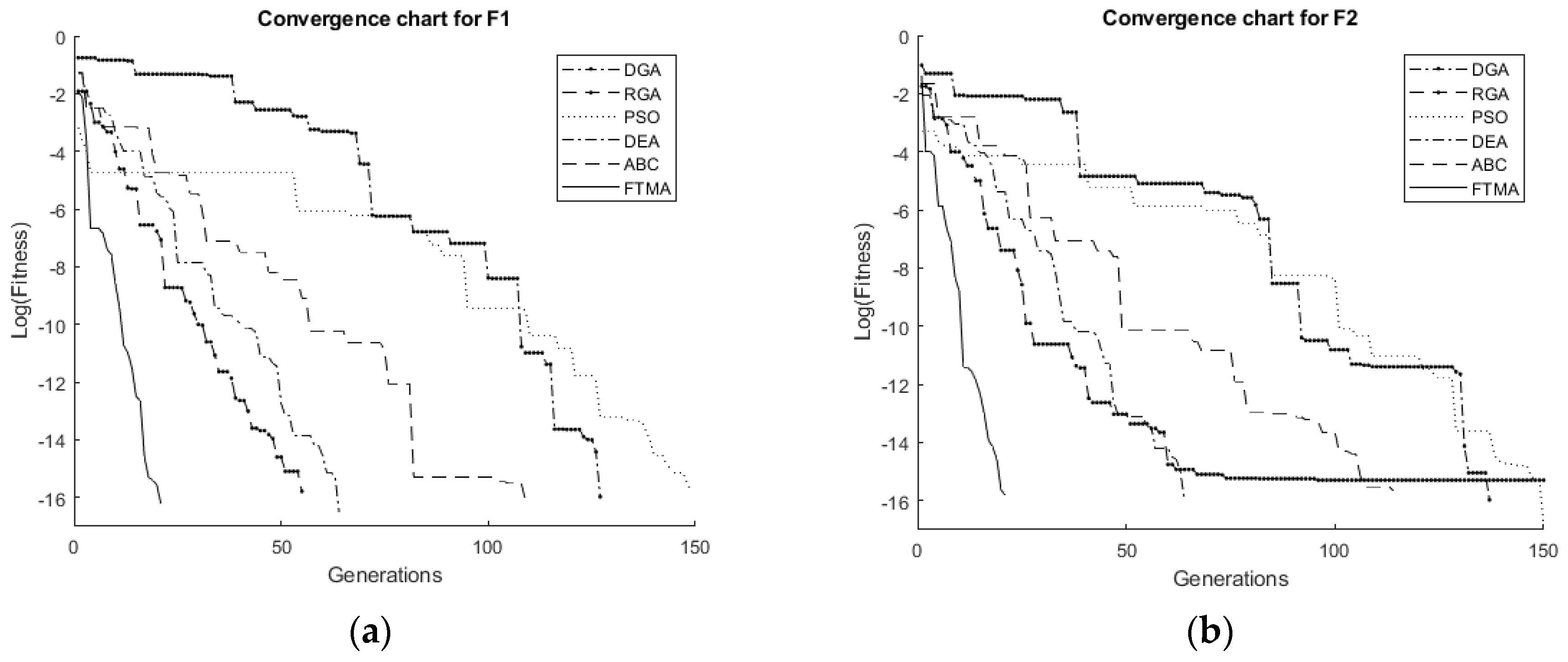
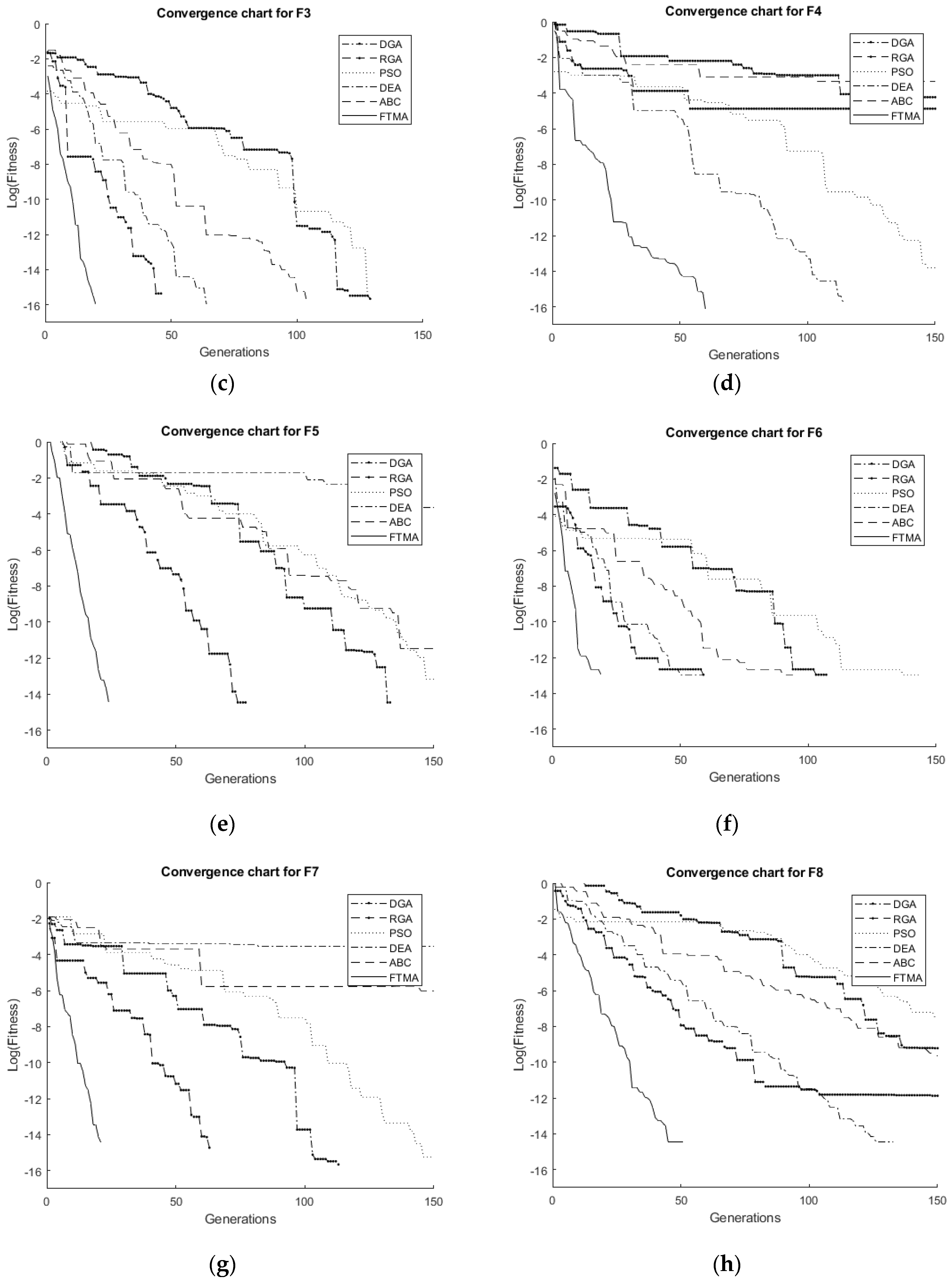
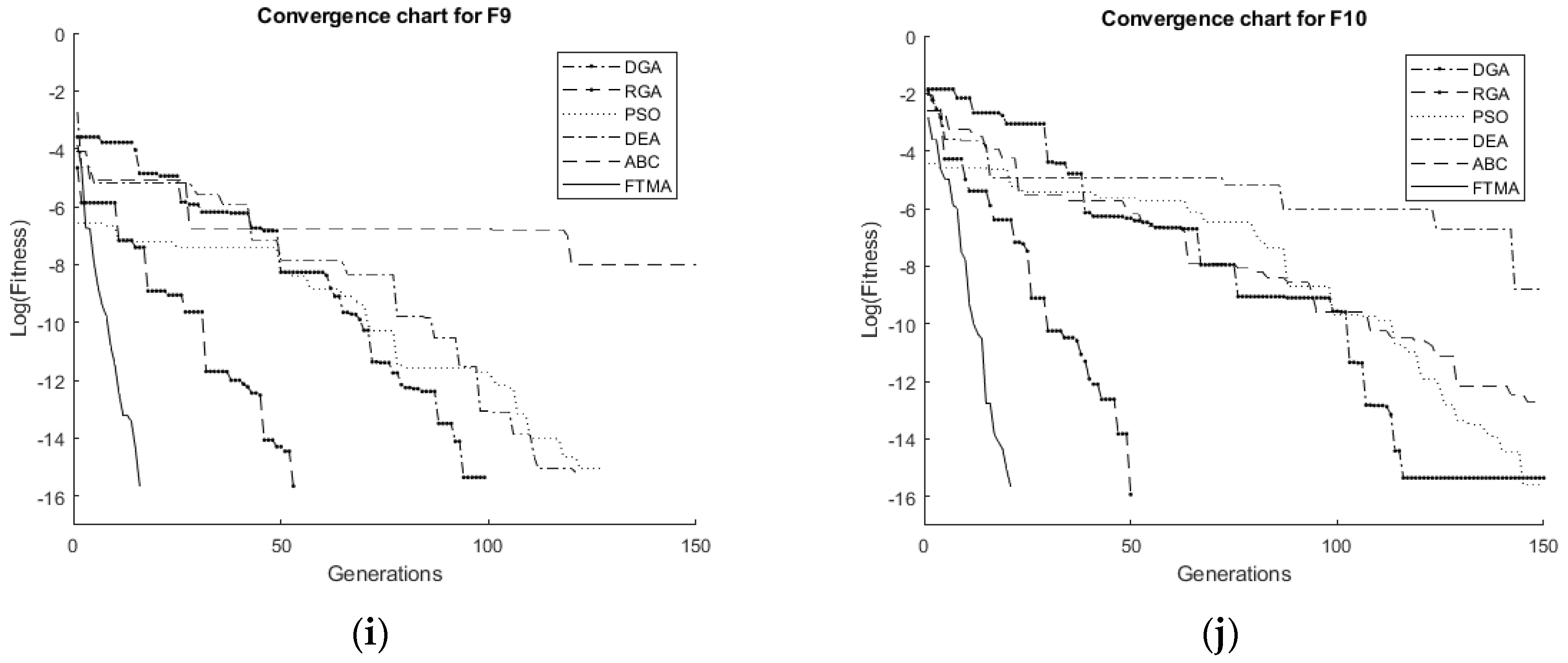
The data represent the output fitness value and the time taken by the optimization algorithm to drive its optimum global fitness below the minimum tolerance error $\epsilon =2.22\times {10}^{-16}$. The data in bold represents the algorithm that simultaneously scored the fastest time and found the global minimum for a specific benchmark function. The underlined data represents the algorithms that failed to pass the tolerance and completed all 1000 generation cycles. The following ten figures in Figure 2 represent the ten benchmark functions, illustrating the process of the optimization. All charts contain six lines which differ in pattern, one for each optimization algorithm.

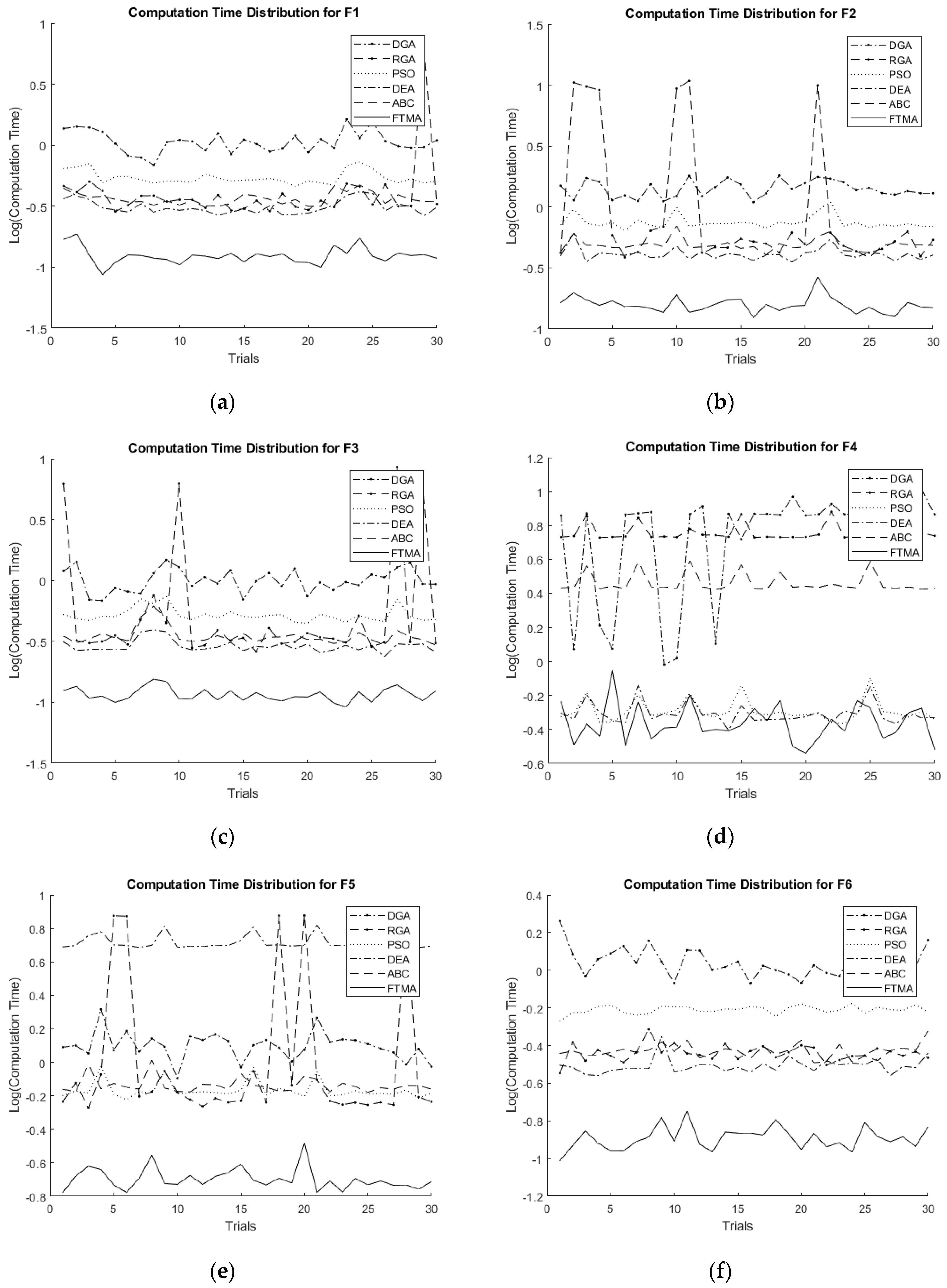
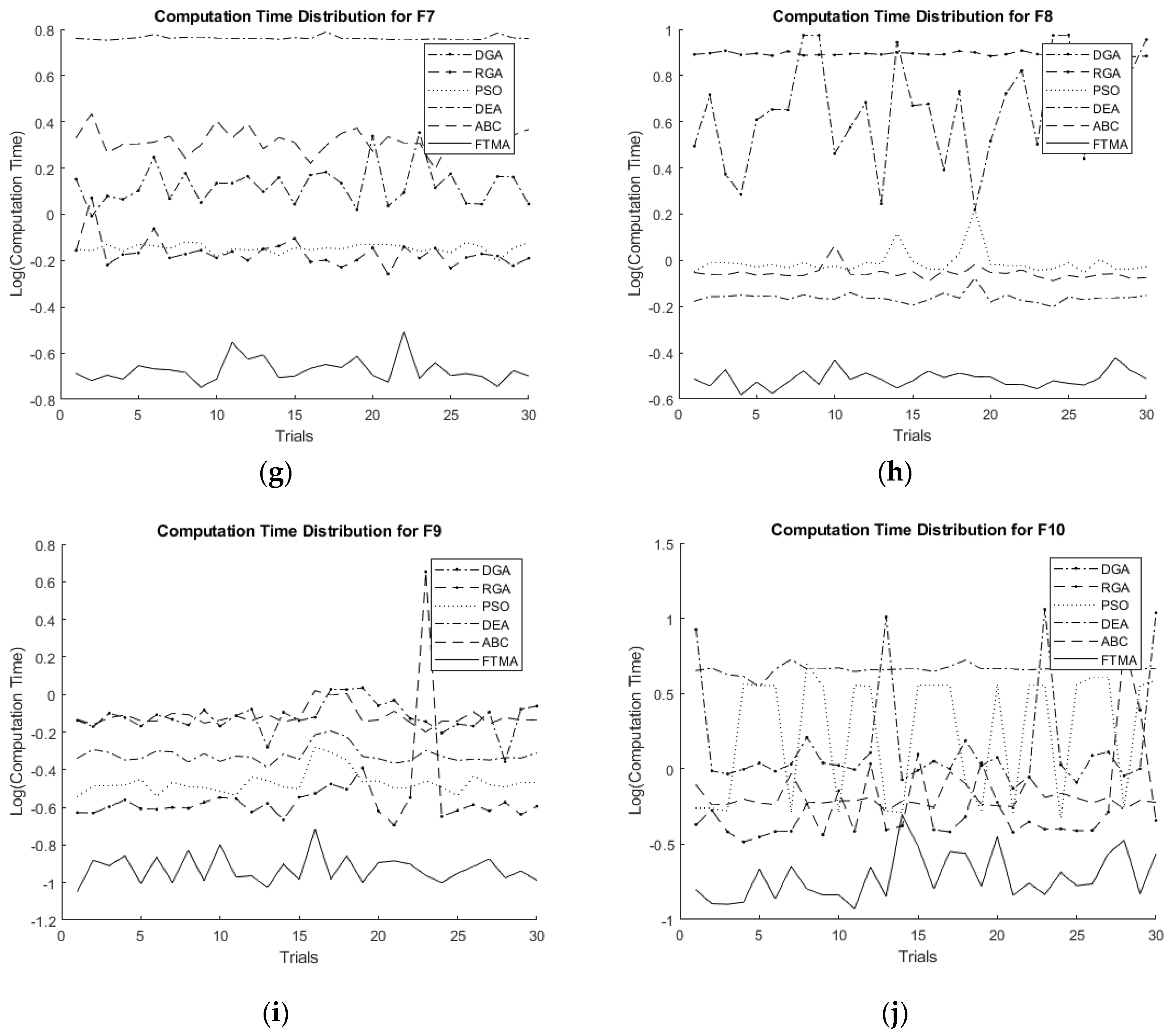
Concerning the computation time, it is evident from Table 3 that the FTMA outperforms all other algorithms. Furthermore, we can see that the DGA failed to reach the optimum in F4 and barely in F7. For RGA, F2, F4, and F8 also failed. PSO evaded all local minima in all the benchmark functions. Furthermore, DEA failed in F10 along with F5 and F7. The ABC algorithm succeeded in avoiding local minima except for F4. In F5, F6, F8, and F9, most of the algorithms succeeded in capturing the zero global optimum value. However, FTMA never fell into the local minima, scoring the best convergence time out of all the optimization algorithms. Additionally, it reaches zero optimum value in the functions from F5 through F9. One can see that some of the optimization algorithms are suitable for some problems and not ideal for others. For example, DGA, RGA, and ABC failed in F4, but DEA succeeded; the situation is in contrary to F5. This confirms the no-free-lunch theorems of the absence of a universal algorithm for every problem. PSO, as well as FTMA, have both succeeded in evading the local maxima and converging to the global one. However, the time taken by PSO to reach the optimum is three to four times the time taken by FTMA. If we look at the ten subgraphs, which represent the search progression of the algorithms for one trial (its results are illustrated in Table 3), we find that the FTMA line (solid black) is the closest line to the vertical axis, which is the logarithmic scale of the global fitness against the number of generations. Although the maximum number of iterations is 1000, the maximum number of iterations displayed in the plots is set to be 150, because most of the algorithms catch the global optimum at or before this generation. In all figures, FTMA is the best-performing function. PSO and ABC are next best in most of the graphs. DGA, RGA, and DEA failed on many occasions. If we take the time which FTMA reached the critical error tolerance, the best of the other functions barely reached the fitness value at the same time. It can be seen from the plots that some of the algorithms have trapped in local minima, especially in F4. This implies that FTMA has the fastest convergence speed among the identified optimization algorithms. The values of the mean and standard deviation for the 30 trials are evaluated for each optimization algorithm and benchmark function.

Table 4. Statistical results of the output error for 30 trials.

Fn.	DGA		RGA		PSO		DEA		ABC		FTMA
	m.	Std.	m.	Std.	m.	Std.	m.	Std.	m.	Std.	m.	Std.
F1	5.94 × 10−17	5.84 × 10−17	5.10 × 10−15	2.43 × 10−14	1.03 × 10−16	6.23 × 10−17	9.13 × 10−17	5.75 × 10−17	1.00 × 10−16	6.80 × 10−17	7.84 × 10−17	5.35 × 10−17
F2	6.29 × 10−17	5.46 × 10−17	2.20 × 10−16	7.04 × 10−16	7.74 × 10−17	5.98 × 10−17	1.05 × 10−16	6.76 × 10−17	8.78 × 10−17	6.24 × 10−17	9.95 × 10−17	6.52 × 10−17
F3	1.29 × 1016	9.96 × 10−17	2.77 × 10−15	1.31 × 10−14	1.36 × 10−16	7.94 × 10−17	1.25 × 10−16	7.97 × 10−17	1.14 × 10−16	7.29 × 10−17	1.03 × 10−16	8.56 × 10−17
F4	2.69 × 10−06	8.17 × 10−06	3.51 × 10−05	0.0001	1.07 × 10−16	6.38 × 10−17	1.09 × 10−16	6.92 × 10−17	1.05 × 10−06	1.85 × 10−06	1.25 × 10−16	6.43 × 10−17
F5	0	0	8.52*10−15	4.52 × 10−14	0	0	3.99 × 10−07	4.84 × 10−07	0	0	0	0
F6	0	0	0	0	0	0	0	0	0	0	0	0
F7	1.18*10−16	1.03*10−16	1.33 × 10−16	8.78 × 10−17	1.03 × 10−16	8.56 × 10−17	1.50 × 10−07	1.96 × 10−07	1.11 × 10−16	9.50 × 10−17	1.03 × 10−16	8.56 × 10−17
F8	2.36*10−16	8.86*10−16	1.59 × 10−08	4.54 × 10−08	0	0	0	0	0	0	0	0
F9	1.03*10−16	1.10*10−16	1.55 × 10−16	1.01 × 10−16	1.25 × 10−16	1.1 × 10−16	1.55 × 10−16	1.01 × 10−16	1.48 × 10−16	1.04 × 10−16	1.40 × 10−16	1.07 × 10−16
F10	6.56*10−16	9.14*10−17	1.19 × 10−16	1.11 × 10−16	3.73 × 10−16	3.01 × 10−16	1.41 × 10−09	6.34 × 10−09	1.04 × 10−16	6.07 × 10−17	9.80 × 10−17	5.83 × 10−17

illustrates the distribution of the output error, and

Table 5. Statistical results of the computation time (seconds) for 30 trials.

Fn.	DGA		RGA		PSO		DEA		ABC		FTMA
	m.	Std.	m.	Std.	m.	Std.	m.	Std.	m.	Std.	m.	Std.
F1	1.085	0.221	0.566	1.091	0.546	0.072	0.315	0.047	0.364	0.040	0.125	0.021
F2	1.423	0.221	2.389	3.780	0.754	0.103	0.413	0.052	0.490	0.063	0.159	0.026
F3	1.021	0.219	1.215	2.224	0.525	0.075	0.291	0.034	0.353	0.067	0.166	0.015
F4	6.299	2.660	5.747	0.658	0.518	0.087	0.500	0.076	2.920	0.410	0.449	0.126
F5	1.275	0.247	1.788	2.561	0.687	0.091	5.200	0.500	0.733	0.084	0.203	0.033
F6	1.122	0.202	0.365	0.037	0.617	0.030	0.312	0.032	0.372	0.032	0.129	0.018
F7	1.361	0.290	0.686	0.110	0.714	0.030	5.783	0.111	2.100	0.241	0.213	0.028
F8	5.055	2.518	7.832	0.124	0.984	0.147	0.691	0.035	0.811	0.059	0.307	0.026
F9	0.773	0.139	0.404	0.761	0.343	0.054	0.478	0.051	0.765	0.092	0.119	0.022
F10	2.288	3.154	0.785	1.188	2.460	1.585	4.583	0.300	0.643	0.110	0.124	0.055

shows the distribution of computation time. The bold and underlined values represent the fastest and failed sets of trials, respectively. The trial sets are presented in ten sub-figures in Figure 3, one for each benchmark function.

In Table 4, the overall trials show that some algorithms that succeeded in one of the tests might not achieve well in another one. It can be concluded that RGA failed in F2; DGA, RGA, and ABC failed in F4. Moreover, DEA failed in F5; DEA, and ABC failed in F7; DGA and RGA failed in F8; while PSO failed in the proposed benchmark function F10, which succeeded in all the other functions. Although DGA average error is slightly less than the mean error of FTMA in F1, F2, and F9, the average computation time is about eight times the computation time of the proposed algorithm. This implies that the proposed algorithm succeeded in reaching the global minimum before DGA. It can be seen that the computation time for the proposed algorithm is the best for all the benchmark functions. In Figure 3, the plots contain six lines with different patterns, one for each optimization algorithm. The figures show the logarithm of the computation time against computation trials. One can determine from these plots that some optimization functions are suitable for some algorithms and not for another. For instance, DEA is suitable for F4 but not for F5. The proposed algorithm always has the best computation time among all the remaining algorithms. Its solid line lies in the bottom near the horizontal axis. In F4, it is accompanied by PSO and DEA; in the other plots, it was alone in the bottom. For the proposed benchmark system, DEA was the worst. PSO fell in local optima many times, and DGA a few times. ABC and RGA performed well, but FTMA was the best.

6. Conclusions

This paper proposed a new global optimization named the fine-tuning meta-heuristic algorithm (FTMA). From the simulation results, it can be concluded that the FTMA reaches the optimum value faster than any other optimization algorithm used in the comparison. Its performance is competing with state-of-the-art methods, namely, RGA, DEA, ABC, PSO, and DGA. It accomplishes this in real-time and, unlike other optimization algorithms, evading any local optima. Moreover, it maintains the accuracy and robustness at the least runtime. Therefore, the FTMA offers a promising approach which, thanks to its rapid convergence time, could be applied in more complicated real-time systems where the time is a crucial factor. This result does not mean that this algorithm can solve any real problem we may encounter in practice, as it stated in the no-free-lunch theorems, there may be processes that this algorithm struggles to solve. So, there are possible opportunities to enhance the FTMA and/or its counterparts. Future studies include using the FTMA in combinatorial optimization or integrating the FTMA in control applications as an online or offline tuning algorithm for finding the optimal parameters of the feedback controllers. Moreover, because the lack of resources (supercomputers, etc.), the computation time of more than two parameters in the algorithm takes hours or sometimes days. So, it is intended to make the problem space higher if these resources become available. Finally, checking multi-dimensional spaces and using multi-objective problem scenarios are possible aspects for future research.

References

1. Goldberg, D. Genetic Algorithms in Search, Optimization and Machine Learning, 1st ed.; Addison-Wesley Longman Publishing Co., Inc.: Boston, MA, USA, 1989. [Google Scholar]
2. Kirkpatrick, S.; Gelatt, C.; Vecchi, M. Optimization by simulated annealing. Science 1983, 220, 671–680. [Google Scholar] [CrossRef] [PubMed]
3. Dorigo, M.; Maniezzo, V.; Colorni, A. Ant system: Optimization by a colony of cooperating agents. IEEE Trans. Syst. Man Cybern. Part B (Cybern.) 1996, 26, 29–41. [Google Scholar] [CrossRef] [PubMed]
4. Eberhart, R.; Kennedy, J. A new optimizer using particle swarm theory. In Proceedings of the Sixth International Symposium on Micro Machine and Human Science, MHS’95, Nagoya, Japan, 4–6 October 1995; IEEE: Piscataway, NJ, USA, 1995; pp. 39–43. [Google Scholar]
5. Karaboga, D.; Basturk, B. A powerful and efficient algorithm for numerical function optimization: Artificial bee colony (ABC) algorithm. J. Glob. Optim. 2007, 39, 459–471. [Google Scholar] [CrossRef]
6. Storn, R.; Price, K. Differential evolution—A simple and efficient heuristic for global optimization over continuous spaces. J. Glob. Optim. 1997, 11, 341–359. [Google Scholar] [CrossRef]
7. Xing, B.; Gao, W. Innovative Computational Intelligence: A Rough Guide to 134 Clever Algorithms, 1st ed.; Springer: Berlin/Heidelberg, Germany, 2016. [Google Scholar]
8. Ibraheem, I.K.; Ajeil, F.H. Path Planning of an autonomous Mobile Robot using Swarm Based Optimization Techniques Technique. Al-Khwarizmi Eng. J. 2016, 12, 12–25. [Google Scholar] [CrossRef]
9. Ibraheem, I.K.; Al-hussainy, A.A. Design of a Double-objective QoS Routing in Dynamic Wireless Networks using Evolutionary Adaptive Genetic Algorithm. Int. J. Adv. Res. Comput. Commun. Eng. 2015, 4, 156–165. [Google Scholar]
10. Ibraheem, I.K.; Ibraheem, G.A. Motion Control of an Autonomous Mobile Robot using Modified Particle Swarm Optimization Based Fractional Order PID Controller. Eng. Technol. J. 2016, 34, 2406–2419. [Google Scholar]
11. Humaidi, A.J.; Ibraheem, I.K.; Ajel, A.R. A Novel Adaptive LMS Algorithm with Genetic Search Capabilities for System Identification of Adaptive FIR and IIR Filters. Information 2019, 10, 176. [Google Scholar] [CrossRef]
12. Humaidi, A.; Hameed, M. Development of a New Adaptive Backstepping Control Design for a Non-Strict and Under-Actuated System Based on a PSO Tuner. Information 2019, 10, 38. [Google Scholar] [CrossRef]
13. Allawi, Z.T.; Abdalla, T.Y. A PSO-Optimized Reciprocal Velocity Obstacles Algorithm for Navigation of Multiple Mobile Robots. Int. J. Robot. Autom. 2015, 4, 31–40. [Google Scholar] [CrossRef]
14. Allawi, Z.T.; Abdalla, T.Y. An ABC-Optimized Type-2 Fuzzy Logic Controller for Navigation of Multiple Mobile Robots Ziyad. In Proceedings of the Second Engineering Conference of Control, Computers and Mechatronics Engineering, Baghdad, Iraq, February 2014; pp. 239–247. [Google Scholar]
15. Tarasewich, P.; McMullen, P. Swarm intelligence: Power in numbers. Commun. ACM 2002, 45, 62–67. [Google Scholar] [CrossRef]
16. Crepinsek, M.; Liu, S.; Mernik, M. Exploration and exploitation in evolutionary algorithms: A survey. ACM Comput. Surv. 2013, 45, 35. [Google Scholar] [CrossRef]
17. Chen, J.; Xin, B.; Peng, Z.; Dou, L.; Zhang, J. Optimal contraction theorem for exploration and exploitation tradeoff in search and optimization. IEEE Trans. Syst. Man Cybern. Part A Syst. Hum. 2009, 39, 680–691. [Google Scholar] [CrossRef]
18. Wolpert, D.; Macready, W. No free lunch theorems for optimization. IEEE Trans. Evol. Comput. 1997, 1, 67–82. [Google Scholar] [CrossRef] [Green Version]
19. Yang, X.S. Firefly algorithms for multimodal optimisation. In Proceedings of the Fifth Symposium on Stochastic Algorithms, Foundations and Applications, Sapporo, Japan, 26–28 October 2009; Watanabe, O., Zeugmann, T., Eds.; Springer: Berlin/Heidelberg, Germany, 2009; Volume 5792, pp. 169–178, Lecture notes in computer, science. [Google Scholar]
20. Yang, X.S.; Deb, S. Cuckoo Search via Lévy flights. In Proceedings of the 2009 World Congress on Nature & Biologically Inspired Computing (NaBIC), Coimbatore, India, 9–11 December 2009; IEEE: Piscataway, NJ, USA, 2009; pp. 210–214. [Google Scholar]
21. Yang, X.S. A new Meta-heuristic bat-inspired algorithm. In Nature Inspired Cooperative Strategies for Optimization (NISCO 2010); Studies in computational intelligence; Springer: Berlin, Germany, 2010; pp. 65–74. [Google Scholar]
22. Yang, X.S. Flower pollination algorithm for global optimization. In Unconventional Computation and Natural Computation; Lecture notes in computer science; Springer: Berlin/Heidelberg, Germany, 2012; Volume 7445, pp. 240–249. [Google Scholar]
23. Yang, X.S. Nature-Inspired Optimization Algorithms, 1st ed.; Elsevier: London, UK, 2014. [Google Scholar]
24. Mirjalili, S.A.; Mirjalili, S.M.; Lewis, A. Grey Wolf Optimizer. Adv. Eng. Softw. 2014, 69, 46–61. [Google Scholar] [CrossRef] [Green Version]
25. Mirjalili, S.A. Moth-flame optimization algorithm: A novel nature-inspired heuristic paradigm. Knowl. Based Syst. 2015, 89, 228–249. [Google Scholar] [CrossRef]
26. Mirjalili, S.A. The Ant Lion Optimizer. Adv. Eng. Softw. 2015, 83, 80–98. [Google Scholar] [CrossRef]
27. Mirjalili, S.A. SCA: A Sine Cosine Algorithm for solving optimization problems. Knowl. Based Syst. 2016, 96, 120–133. [Google Scholar] [CrossRef]
28. Mirjalili, S.A.; Lewis, A. The Whale Optimization Algorithm. Adv. Eng. Softw. 2016, 95, 51–67. [Google Scholar] [CrossRef]
29. Lee, Y.; Marvin, A.; Porter, S. Genetic algorithm using real parameters for array antenna design optimization. In MTT/ED/AP/LEO Societies Joint Chapter UK and Rep. of Ireland Section. 1999 High Frequency Postgraduate Student Colloquium; Cat. No.99TH840; IEEE: Piscataway, NJ, USA, 1999; pp. 8–13. [Google Scholar]
30. Bessaou, M.; Siarry, P. A genetic algorithm with real-value coding to optimize multimodal continuous functions. Struct. Multidiscip. Optim. 2001, 23, 63–74. [Google Scholar] [CrossRef]
Figure 1. Graph of ALLAWI test function for d = 2 and ε = 2.22 × 10 16 .
Processes 07 00657 g001
Figure 2. Convergence charts for the ten benchmark functions. (a) F1, (b) F2, (c) F3, (d) F4, (e) F5, (f) F6, (g) F7, (h) F8, (i) F9, and (j) F10.
Processes 07 00657 g002aProcesses 07 00657 g002bProcesses 07 00657 g002c
Figure 3. Computation time distribution for the ten benchmark functions. (a) F1, (b) F2, (c) F3, (d) F4, (e) F5, (f) F6, (g) F7, (h) F8, (i) F9, and (j) F10.
Processes 07 00657 g003aProcesses 07 00657 g003b