Improving Flexibility and Energy Efficiency of Post-Combustion CO₂ Capture Plants Using Economic Model Predictive Control

Abstract

To reduce CO${}_2$ emissions from power plants, electricity companies have diversified their generation sources. Fossil fuels, however, still remain an integral energy generation source as they are more reliable compared to the renewable energy sources. This diversification as well as changing electricity demand could hinder effective economical operation of an amine-based post-combustion CO${}_2$ capture (PCC) plant attached to the power plant to reduce CO${}_2$ emissions. This is as a result of large fluctuations in the flue gas flow rate and unavailability of steam from the power plant. To tackle this problem, efficient control algorithms are necessary. In this work, tracking and economic model predictive controllers are applied to a PCC plant and their economic performance is compared under different scenarios. The results show that economic model predictive control has a potential to improve the economic performance and energy efficiency of the amine-based PCC process up to 6% and 7%, respectively, over conventional model predictive control.

1. Introduction

The reliance on fossil fuels, especially coal for electricity, is one of the major causes of increased amount of anthropogenic carbon dioxide in the atmosphere and climate change. At the moment, almost 40% of the world’s energy is produced from combustion of coal [1]. Although renewable energies such as those obtained from wind or solar or biomass can be helpful in reducing CO${}_2$ emissions, they are not mature enough to fully take over. Therefore, for these fossil fuels to keep contributing to the global energy mix, carbon capture and storage (CCS) must be implemented. CCS involves capturing carbon dioxide from large point sources such as power plants, transporting and storing it in deep geological or oceanic wells for a long time in a supercritical state [2]. Among the various options for CO${}_2$ capture, post-combustion CO${}_2$ capture (PCC) using reactive solvents is considered the most mature and viable option as it can easily be retrofitted to existing power plants. However, a major setback to the realization of this technology is its high regeneration heat requirement. Studies have shown that a PCC plant attached to a power plant reduces the power plant’s efficiency from about 40% to 30% [3].

Figure 1 shows an overview of a fossil-fueled power plant with CO${}_2$ capture. In a typical fossil-fueled power plant with CO${}_2$ capture, the fuel is combusted in air to generate flue gas, which is used to generate high pressure steam in the steam generator. The steam is then used to turn a turbine leading to electricity generation. At the same time, part of the steam is sent to the PCC plant for regeneration of the captured CO${}_2$. This results in a reduction of the power plant’s efficiency. The flue gas (containing about 15 mol % CO${}_2$) on the other hand is channeled to the PCC plant for treatment before it is released into the atmosphere. The power plant’s ability to meet the varying demands of the end users while capturing CO${}_2$ is a major concern. This could result in large fluctuations in the flue gas flow rate and the availability of the steam from the power plant to the the capture plant. These fluctuations as well as issues such as complex/nonlinear system dynamics could make attainment of the operational objectives and control of the PCC plant difficult. These challenges have motivated the research on the development of more flexible and economical control for PCC plants.

Ziaii et al. [4] designed a ratio controller to maintain a 90% CO${}_2$ capture efficiency in the absorber. They considered a disturbance in the steam availability to the reboiler and used the liquid to gas flow ratio as the manipulated variable. Lin et al. [5] presented two different PI control strategies to maintain a desired absorption efficiency. They used the lean solvent flow rate and the reboiler heat input as the manipulated variables.

Advanced control algorithms such as Model Predictive Control (MPC) have also been applied to the control of PCC plants. Bedelbayev et al. [6] presented an MPC scheme for the absorber in standalone. Panahi and Skogestad [7,8] implemented an MPC scheme with two controlled variables—the CO${}_2$ recovery and the reboiler temperature. In the context of scheduling and control, He et al. [9] studied the flexibility of a post-combustion CO${}_2$ capture process using MPC. They conducted this study by investigating key process variables such as CO${}_2$ absorption efficiency and CO${}_2$ composition in the product stream in both closed-loop and open-loop. They observed that, under high frequency disturbances in the flue gas flow rate, a well-tuned controller is needed to avoid oscillations in the absorption efficiency. Bankole et al. [10] used a two-level control strategy consisting of an upper-level scheduler and a lower-level supervisory controller to handle the flexible operation of a load-following power plant with CO${}_2$ capture under three different capture scenarios. MacDowell and Shah [11] also evaluated the operation of a PCC plant under four different scenarios—load following, solvent storage, exhaust gas by-pass and time-varying solvent regeneration—using multi-period optimization.

An emerging MPC formulation that has a potential to determine the optimal operating policy directly in the control layer is Economic Model Predictive Control (EMPC). In EMPC, real-time process optimization and feedback control are unified [12]. This means that, in EMPC, an economic cost function or objective is directly optimized instead of tracking a predetermined set-point [13,14]. To date, EMPC has had some successful applications in different processes [15,16,17,18,19]. In the studies of Zeng et al. [15] and Liu et al. [16], for example, EMPC was applied to improve the effluent quality of a waste water treatment process and the operation of an oil sands primary separation vessel, respectively. Idris et al. [17] applied EMPC to a continuous catalytic distillation process whileMendoza-Serrano et al. [18] and Touretzky et al. [19] applied EMPC to temperature control in buildings. In these applications, EMPC showed a potential to significantly improve the performance of the classical MPC. However, it should be pointed out that the reported EMPC designs and their benefits are usually process specific. The general case where EMPC has a clear edge over classical MPC remains to be understood.

In this study, EMPC was applied to a PCC plant attached to a load-following power plant and its performance was compared with classical tracking MPC from different aspects. In particular, the operation of the PCC plant under time-varying flue gas flow rate and steam price was considered. The performance of tracking MPC and EMPC under two different carbon tax policies are investigated namely: without tax-free emission limit and with tax-free emission limit. The rest of the paper is organized as follows: in Section 2, a detailed PCC plant model based on first principles is presented. In Section 3, the designs of both MPC and EMPC as well as their numerical implementation are presented. In Section 4, a systematic investigation of the performance of both MPC and EMPC from different aspects including time-varying conditions and uncertainty is conducted.

2. Model Development

A typical PCC plant is comprised of two major operating units namely, absorption and desorption columns, where reactive separation takes place. A schematic diagram of the PCC plant considered in this work is shown in Figure 2. The process starts in the absorption column where the flue gas (containing high amount of CO${}_2$) from the power plant is contacted with the lean solvent—solvent containing low amount of CO${}_2$ (in this work, state-of-the-art 5 M Monoethanolamine (MEA) is used as solvent)—in a counterclockwise way. The flue gas leaves the absorption column as treated gas with a low amount of CO${}_2$. The solvent with a high amount of CO${}_2$ (rich solvent) exits the absorption column and goes through the lean-rich heat exchanger where it trades heat with the lean solvent exiting the reboiler. The rich solvent enters the desorption unit and contacts hot vapor from the reboiler. In the desorption column, the acid gas (CO${}_2$) is stripped from the rich solvent. Gas with a high concentration of CO${}_2$ (90–99%) exits the desorption column from the top while the solvent moves out of the desorption column to the reboiler. In the reboiler, the solvent is heated to a temperature of about 120 C. The gas exits the reboiler to the desorption column while the lean solvent is recycled to the absorption column for re-absorption. In this work, the lean solvent flow rate and the steam from the power plant are the manipulated variables. The control objective is to reduce CO${}_2$ emissions and heat consumption at a reasonable economic cost. The disturbances are the flue gas flow rate and steam from the power plant.

Several studies on dynamic modelling of the PCC process exist in literature. The model used in this work is based on the work of Harun et al. [20]. However, the lean-rich heat exchanger was modeled using the log-mean temperature approach. In addition, the buffer tank and column heat losses were not considered in this work. The details of the model used in this study are summarized in this section.

2.1. Absorption and Desorption Units

The model formulations for the absorption and desorption units are similar. The differences are the direction of reactions and the presence of reboiler and condenser in the desorption unit.

2.1.1. Modeling Assumptions

The assumptions used in the modeling of the PCC plant are:

• Well mixed bulk and liquid phases. Each stage therefore behaves like a continuously stirred tank reactor (CSTR) with no spacial variation in properties.
• Reactions occur only in the liquid film and the influence of the reaction on mass transfer is described using enhancement factor.
• Mass and heat transfer are described by the two film theory [21].
• Pressure drop in the two columns is linear.
• No heat losses to the surrounding area.

2.1.2. Balance Equations

Equations (1)–(4) describe the mass and heat balances occurring in the two columns. These equations are written along the axis of the columns to determine the axial concentration and temperature profiles. Since the assumption that a stage in both columns is well mixed has been made, there are no radial changes in temperature and concentration in each column:

$$\frac{d{C}_{Li}}{dt}=\frac{4F_L}{\pi D_c^2}\frac{\partial C_{Li}}{\partial l}+(N_i{a}^I),i={\mathrm{CO}}_2,\mathrm{MEA},{\mathrm{H}}_2\mathrm{O},{\mathrm{N}}_2,$$

(1)

$$\frac{d{C}_{Gi}}{dt}=-\frac{4F_G}{\pi D_c^2}\frac{\partial C_{Gi}}{\partial l}-(N_i{a}^I),i={\mathrm{CO}}_2,\mathrm{MEA},{\mathrm{H}}_2\mathrm{O},{\mathrm{N}}_2,$$

(2)

$$\frac{d{T}_L}{dt}=\frac{4F_L}{\pi D_c^2}\frac{\partial T_L}{\partial l}+\frac{(Q_L{a}^I)}{{\sum }_{i=1}^n{C}_{Li}{C}_{p,i}},$$

(3)

$$\frac{d{T}_G}{dt}=-\frac{4F_G}{\pi D_c^2}\frac{\partial T_G}{\partial l}+\frac{(Q_G{a}^I)}{{\sum }_{i=1}^n{C}_{Gi}{C}_{p,i}}.$$

(4)

In Equations (1)–(4) above, $C_i$ is the phase (subscripts L and G are liquid phase and gas phase respectively) concentration of component i in $\mathrm{kmol}/{\mathrm{m}}^3$, F is the phase volumetric flow in ${\mathrm{m}}^3/\mathrm{s}$, $D_c$ is the cross-sectional area of the column in $\mathrm{m}$, $N_i$ is the mass transfer rate in $\mathrm{kmol}/{\mathrm{m}}^2\mathrm{s}$, T is temperature in $\mathrm{K}$, l is the length of the column in $\mathrm{m}$, $C_p$ is the heat capacity in $\mathrm{kJ}/\mathrm{kmol}$, Q is the heat transfer rate in $\mathrm{kJ}/{\mathrm{m}}^2\mathrm{s}$ and $a^I$ is the interfacial area in ${\mathrm{m}}^2/{\mathrm{m}}^3$. In the absorption unit, $F_L$ is a manipulated variable to control the ${\mathrm{CO}}_2$ emission, whereas $F_G$ is a disturbance from the power plant.

2.1.3. Heat and Mass Transfer Rates

The mass transfer rates in the columns are determined using Equation (5):

$$N_i=K_{Gi}{P}_t(y_i-y_i^{\ast }),i={\mathrm{CO}}_2,\mathrm{MEA},{\mathrm{H}}_2\mathrm{O},$$

(5)

where $K_{Gi}$ is the overall mass transfer coefficient in $\mathrm{kmol}/{\mathrm{m}}^3\mathrm{Pa}$, $P_t$ is the stage pressure in $\mathrm{Pa}$, and $y_i$ and $y_i^{\ast }$ are the bulk and equilibrium gas phase component mole fractions. The overall gas phase mass transfer coefficients are used to compute the mass transfer rates between the two phases. This is convenient as it avoids the determination of interfacial concentrations. In this work, the mass transfer rate of ${\mathrm{N}}_2$ is assumed to be zero or negligible.

The interface equilibrium H${}_2$O and MEA concentrations are determined from their saturated vapor pressures as shown in Equation (6), whereas that of CO${}_2$ is determined using Henry’s law as shown in Equation (7):

$$y_i^{\ast }{P}_t=x_i{\gamma }_i{P}_i^v,i={\mathrm{H}}_2\mathrm{O},\mathrm{MEA},$$

(6)

$$y_i^{\ast }{P}_t=H{e}_i{C}_i^{\ast }{\gamma }_i,i={\mathrm{CO}}_2,$$

(7)

where ${\gamma }_i$ is the activity coefficient of component i, $H{e}_i$ is the Henry’s constant and $P_i^v$ is the saturated vapor pressure of component i in $\mathrm{Pa}$.

The overall mass transfer coefficients are determined using Equation (8) below:

$$\frac{1}{K_{Gi}}=\frac{1}{k_{Gi}}+\frac{He}{k_{Li}{E}_f},i={\mathrm{CO}}_2,\mathrm{MEA},{\mathrm{H}}_2\mathrm{O},$$

(8)

where $k_{Gi}$ and $k_{Gi}$ are the gas and liquid mass transfer coefficients of component i, respectively, in $\mathrm{kmol}/{\mathrm{m}}^2\mathrm{s}$ and $E_f$ is the enhancement factor.

The mass transfer coefficients and interfacial area are estimated using Onda’s correlations [22]. The enhancement factor approach is used to determine the influence of the reactions on the rates of mass transfer. The pseudo-first order enhancement factor during absorption is calculated using Equation (9) determined by van Kravelen and Hoftijzer [23]:

$$E=\frac{\sqrt{k_i{D}_i{C}_j}}{k_{L}i},i={\mathrm{CO}}_2,j=\mathrm{MEA},$$

(9)

where $k_i$ is the second order rate constant in ${\mathrm{m}}^3/\mathrm{kmol}$ and $D_i$ is the liquid phase diffusivity of component i in ${\mathrm{m}}^2/\mathrm{s}$. In the case of desorption, the enhancement factor is calculated using Equation (10) [24]:

$$E=1+\frac{(\frac{D_{MEACO{O}^{-}}}{D_{C{O}_2}})\sqrt{K_{eq}{C}_{MEA}^B}}{(1+2(\frac{D_{MEACO{O}^{-}}}{D_{MEA}})\sqrt{K_{eq}{C}_{C{O}_2}^B})(\sqrt{C_{C{O}_2}^B}+\sqrt{C_{C{O}_2}^I})},$$

(10)

where $D_{MEACO{O}^{-}}$, $D_{C{O}_2}$ and $D_{MEA}$ are the liquid phase diffusivities of carbamate ion, CO${}_2$ and MEA respectively in ${\mathrm{m}}^2/\mathrm{s}$, $C_{C{O}_2}^B$ and $C_{MEA}^B$ are the bulk liquid phase concentrations of CO${}_2$ and MEA respectively in $\mathrm{kmol}/{\mathrm{m}}^3$, $C_{C{O}_2}^I$ is the concentration of CO${}_2$ at the gas–liquid interface in $\mathrm{kmol}/{\mathrm{m}}^3$, and $K_{eq}$ is the overall equilibrium rate constant in ${\mathrm{m}}^3/\mathrm{kmol}$.

The heat transfer rates across the interface for gas and liquid phases are determined using Equations (11) and (12), respectively. The heat of reaction is accounted for in the liquid heat transfer rate computation:

$$Q_G=h_{GL}(T_L-T_G),$$

(11)

$$Q_L=h_{GL}(T_L-T_G)+\Delta H_{rxn}{N}_{C{O}_2}+\Delta H_{vap}{N}_{H_{2}O},$$

(12)

where $h_{GL}$ is the gas–liquid heat transfer coefficient in $\mathrm{kJ}/{\mathrm{m}}^2\mathrm{s}$, $\Delta H_{rxn}$ is the heat of reaction between MEA and CO${}_2$ in $\mathrm{kJ}/{\mathrm{m}}^3\mathrm{s}$ and $\Delta H_{vap}$ is the heat of vaporization of H${}_2$O in $\mathrm{kJ}/{\mathrm{m}}^3\mathrm{s}$. The gas–liquid heat transfer coefficient was determined using the Chilton–Colburn analogy [25].

2.2. Heat Exchanger Model

The heat exchanger, especially the lean-rich heat exchanger, is a crucial component of the post combustion capture plant. It seeks to make the process heat efficient by taking heat from the hot lean solvent (source) to the cool rich solvent (sink) exiting the absorber. Since there is no movement of mass from one stream to the other and no accumulation is assumed, the mass balances are not considered in the heat exchanger model.

2.2.1. Energy Balance

The energy balance equations are shown in Equations (13) and (14):

$$\frac{d{T}_{tube}}{dt}=\frac{{\dot{V}}_{tube}}{V_{tube}}(T_{tube,in}-T_{tube,out})+\dot{Q}\frac{1}{{\widehat{Cp}}_{tube}{\rho }_{tube}{V}_{tube}},$$

(13)

$$\frac{d{T}_{shell}}{dt}=\frac{{\dot{V}}_{shell}}{V_{shell}}(T_{shell,in}-T_{shell,out})+\dot{Q}\frac{1}{{\widehat{Cp}}_{shell}{\rho }_{shell}{V}_{shell}},$$

(14)

where T is the temperature in $\mathrm{K}$, $\dot{V}$ is the volumetric flow rate in ${\mathrm{m}}^3/\mathrm{s}$, V is the volume in ${\mathrm{m}}^3$, $\dot{Q}$ is the heat transfer rate in $\mathrm{kJ}/\mathrm{s}$, $\widehat{Cp}$ is the average molar liquid heat capacity in $\mathrm{kJ}/\mathrm{kmol}$, $\rho$ is the average molar density in $\mathrm{kmol}/{\mathrm{m}}^3$ and $\Delta T_{LMTD}$ is the log-mean temperature difference between the hot side and the cold side of the heat exchanger in $\mathrm{K}$. Subscripts $tube$, $shell$, $in$ and $out$ represent the tube-side, shell-side, inlets and outlets of the heat exchanger, respectively.

The log-mean temperature difference between the shell-side and tube-side was determined using Equation (15) below:

$$\dot{Q}=UA\Delta T_{LMTD},$$

(15)

$$\Delta T_{LMTD}=\frac{\Delta T_1-\Delta T_2}{ln(\Delta T_1/\Delta T_2)},$$

(16)

where $\Delta T_1$ and $\Delta T_2$ are equal to ($T_{shell,in}-T_{tube,out}$) and ($T_{shell,out}-T_{tube,in}$), respectively.

2.3. Reboiler Model

The reboiler is the most heat-intensive part of the plant. In this unit, the rich solvent is heated to break the chemical bonds between CO${}_2$ and MEA. H${}_2$O, CO${}_2$ and MEA are vaporized in the process and channeled to the bottom of the desorption unit. The solvent containing low amount of the acid gas (CO${}_2$) exits the unit as lean solvent.

2.3.1. Material Balance

The material balance around the reboiler is shown in Equation (17):

$$\frac{d{M}_i}{dt}=F_{in}{x}_{i,in}-V{y}_{i,out}-L{x}_{i,out},i={\mathrm{CO}}_2,{\mathrm{MEAH}}_2\mathrm{O},$$

(17)

where $M_i$ is the mass holdup of component i in $\mathrm{kmol}$, F is the molar flow rate in $\mathrm{kmol}/\mathrm{s}$, V and L are the vapor and liquid flow rates, respectively, in $\mathrm{kmol}/\mathrm{s}$. The subscripts $in$ and $out$ denote inlet and outlet streams, respectively. In this study, we assumed that the liquid level and the reboiler pressure does not change. Thus, there is no vapour or liquid holdup.

2.3.2. Energy Balance

The energy balance equation is shown in Equation (18):

$$\rho C_{p}V\frac{d{T}_{reb}}{dt}=F_{in}{x}_{in}-V{H}_{v,out}-L{H}_{L,out}+Q_{reb},$$

(18)

where $T_{reb}$ is the temperature in $\mathrm{K}$, $\rho$ is the density in $\mathrm{kmol}/{\mathrm{m}}^3$, $C_p$ is the molar heat capacity in $\mathrm{kJ}/\mathrm{kmol}$, V is the holdup volume in ${\mathrm{m}}^3$, H is the enthalpy in $\mathrm{kJ}$ and $Q_{reb}$ is the heat input in $\mathrm{KJ}/\mathrm{s}$. $Q_{reb}$ is used as a manipulated variable to control the reboiler temperature.

2.4. Physical and Chemical Properties

The accuracy of process models hinges on accurate predictions of the physical and chemical properties of the system. The non-ideal liquid phase behaviour of the CO${}_2$-MEA-H${}_2$O system was modeled using the electrolyte Non-Random Two Liquids (eNRTL) thermodynamic model. The liquid phase activity coefficients were obtained from Aspen Properties (version 9.0, Aspen Technology, Inc., Bedford, Massachusetts 01730, USA) and implemented via look-up tables. The gas phase behaviour was modeled as an ideal phase. The heat and mass transfer coefficients of the two phases are dependent on several property calculations such as diffusivity, viscosity, specific heat capacity, density and several other correlations. These correlations as well as the kinetic parameters for the CO${}_2$-MEA-H${}_2$O system used in this work can be found in the work of Harun [26].

2.5. Model Discretization

The partial differential equations in the column equations are converted to ordinary differential equations using the method of lines. This results in the conversion of the derivatives with respect to the length of the column being discretized into five stages, thus rendering the partial differential equations as ordinary differential equations. After discretization, the model described in this section can be written in a compact form as shown in the system of Differential Algebraic Equations (DAEs) below:

$$\begin{array}{c}\hfill \dot{x}=f(x,z,u,p),\end{array}$$

(19)

$$\begin{array}{c}\hfill g(x,z,u,p)=0,\end{array}$$

(20)

$$\begin{array}{c}\hfill y=h(x,z,u,p),\end{array}$$

(21)

where $x\in {\mathbb{R}}^{103}$ denotes the differential states, $z\in {\mathbb{R}}^7$ denotes the algebraic states, $u=[F_L,Q_{reb}]$ denotes the manipulated input solvent flow rate in $\mathrm{L}/\mathrm{s}$ and reboiler heat input in $\mathrm{MW}$, $p=\left[F_G\right]$ denotes the uncontrolled input flue gas flow rate, $y=[y_{C{O}_2},T_{reb}]$ denotes the outputs CO${}_2$ flow rate in the treated gas in $\mathrm{kg}/\mathrm{h}$ and reboiler temperature in $\mathrm{K}$. The system of DAEs described in Equations (19) – (21) will be used in the MPC and EMPC designs.

3. Control Problem Formulation and Design

In this work, two control objectives are considered. The first is reduction of the amount of CO${}_2$ released into the atmosphere. The second control objective is the minimization of the heat consumed at the regeneration section of the plant. In the case of MPC, these objectives have been translated to tracking the optimal CO${}_2$ emission and reboiler temperature. Hard constraints are imposed to ensure that the temperature of the solvent in the reboiler does not go beyond the point where the solvent degrades (120 C). The designed controller must achieve these two control objectives while rejecting disturbances in the form of fluctuations in the flue gas flow rate originating from the power plant and time-varying steam price due to the time-varying electricity demand.

3.1. Conventional Set-Point Tracking MPC

To operate chemical plants in a time-varying manner, process economic optimization and control are usually decomposed into a hierarchical structure or layer. In this work, the conventional set-point tracking MPC takes a two-step approach, namely: steady-state optimization (SSO) and dynamic tracking. First, a steady-state optimization is performed to determine the optimal operating point for MPC. The optimization problem is as follows:

Optimization problem 1. Steady-state optimization problem

$$\begin{array}{cc}\hfill \underset{x_s,z_s,u_s,ϵ}{min}& l={\alpha }_1{u}_{2,s}+{\alpha }_2ϵ,\hfill \end{array}$$

(22)

$$\begin{array}{cc}\hfill \mathrm{s}.\mathrm{t}.& f(x_s,z_s,u_s,p)=0,\hfill \end{array}$$

(23)

$$\begin{array}{cc}\hfill & g(x_s,z_s,u_s,p)=0,\hfill \end{array}$$

(24)

$$\begin{array}{cc}\hfill & y_s=h(x_s,z_s,u_s,p),\hfill \end{array}$$

(25)

$$\begin{array}{cc}\hfill & y_{1,s}-y_{limit}\le ϵ,\hfill \end{array}$$

(26)

$$\begin{array}{cc}\hfill & ϵ\ge 0,\hfill \end{array}$$

(27)

$$\begin{array}{cc}\hfill & 385.15\le y_{2,s}\le 393.15,\hfill \end{array}$$

(28)

$$\begin{array}{cc}\hfill & 0.1\le u_{1,s}\le 2.0,\hfill \end{array}$$

(29)

$$\begin{array}{cc}\hfill & 0.05\le u_{2,s}\le 0.5,\hfill \end{array}$$

(30)

where $y_{limit}$ is the threshold value of CO${}_2$ above which cost will be incurred in kg/h, $ϵ$ is a variable which represents the amount of CO${}_2$ released above the threshold value in kg/h, and ${\alpha }_1$ indicates the price of steam from the power plant, whereas ${\alpha }_2$ is the carbon price/tax.

Equation (22) is the economic cost function, Equations (23)–(25) are the steady-state of Equations (19)–(21) described in Section 2 in compact form, and Equations (26) and (27) form a soft constraint on the CO${}_2$ emissions. Equations (28)–(30) are hard constraints on the reboiler temperature, solvent flow rate and reboiler heat input, respectively. The constraint on the reboiler temperature is to ensure that the temperature does not fall below the minimum CO${}_2$ regeneration temperature or go beyond the degradation temperature of the solvent.

MPC is an optimal control strategy that has gained popularity in the chemical process industry. The MPC controller is designed to track a predetermined optimal steady-state value. The cost function is quadratic and penalizes the deviations of the state and input trajectories from the set-point. The MPC used in this work takes the form shown below:

Optimization problem 2. Tracking MPC optimization problem

$$\begin{array}{cc}\hfill \underset{u(t)\in S(\Delta )}{min}& {\int }_{t_k}^{t_{k+N_p}}({(y_s-\tilde{y}(t))}^{T}Q(y_s-\tilde{y}(t))+{(u_s-u(t))}^{T}R(u_s-u(t)))dt,\hfill \end{array}$$

(31)

$$\begin{array}{cc}\hfill \mathrm{s}.\mathrm{t}.& \dot{\tilde{x}}=f(\tilde{x}(t),\tilde{z}(t),u(t),p(t)),\hfill \end{array}$$

(32)

$$\begin{array}{cc}\hfill & g(\tilde{x}(t),\tilde{z}(t),u(t),p(t))=0,\hfill \end{array}$$

(33)

$$\begin{array}{cc}\hfill & \tilde{y}=h(\tilde{x}(t),\tilde{z}(t),u(t),p(t)),\hfill \end{array}$$

(34)

$$\begin{array}{cc}\hfill & \tilde{x}(t_k)=x(t_k),\hfill \end{array}$$

(35)

$$\begin{array}{cc}\hfill & 385.15\le {\tilde{y}}_2(t)\le 393.15,\hfill \end{array}$$

(36)

$$\begin{array}{cc}\hfill & 0.1\le u_1(t)\le 2.0,\hfill \end{array}$$

(37)

$$\begin{array}{cc}\hfill & 0.05\le u_2(t)\le 0.5,\hfill \end{array}$$

(38)

where $S(\Delta )$ is the family of piece-wise constant functions with a sampling time $\Delta$, $N_p$ is the prediction horizon, $\tilde{x}$, $\tilde{y}$ and $\tilde{z}$ denote the predicted differential, output and algebraic states, respectively. Q and R are the weighting matrices on the outputs and control actions, respectively. Their determination and values are described in the results section.

In Optimization problem 2, Equation (31) is the cost function; Equations (32)–(34) represent the PCC model; Equation (35) is the initial condition of the system at time instant $t_k$; and Equations (36)–(38) are the same as the constraints in Optimization problem 1. At the next sampling time, Optimization problem 2 is solved again. This forms an implicit feedback control law.

3.2. Economic Model Predictive Control

EMPC integrates steady-state optimization and dynamic tracking by directly optimizing economic performance in the dynamic control problem. The difference between MPC and EMPC is the cost function. While MPC uses a quadratic cost function and require set-point updating, EMPC uses a general economic cost function and does not require any set-points.

The EMPC at time instant $t_k$ is formulated as the optimization problem below:

Optimization problem 3. EMPC optimization problem

$$\begin{array}{cc}\hfill \underset{u(t)\in S(\Delta )}{min}& {\int }_{t_k}^{t_{k+N_p}}({\alpha }_1(t)u_2(t)+{\alpha }_2ϵ(t))dt,\hfill \end{array}$$

(39)

$$\begin{array}{cc}\hfill \mathrm{s}.\mathrm{t}.& \dot{\tilde{x}}=f(\tilde{x}(t),\tilde{z}(t),u(t),p(t)),\hfill \end{array}$$

(40)

$$\begin{array}{cc}\hfill & g(\tilde{x}(t),\tilde{z}(t),u(t),p(t))=0,\hfill \end{array}$$

(41)

$$\begin{array}{cc}\hfill & \tilde{y}=h(\tilde{x}(t),\tilde{z}(t),u(t),p(t)),\hfill \end{array}$$

(42)

$$\begin{array}{cc}\hfill & \tilde{x}(t_k)=x(t_k),\hfill \end{array}$$

(43)

$$\begin{array}{cc}\hfill & {\tilde{y}}_1(t)-y_{limit}\le ϵ(t),\hfill \end{array}$$

(44)

$$\begin{array}{cc}\hfill & ϵ(t)\ge 0,\hfill \end{array}$$

(45)

$$\begin{array}{cc}\hfill & 385.15\le {\tilde{y}}_2(t)\le 393.15,\hfill \end{array}$$

(46)

$$\begin{array}{cc}\hfill & 0.1\le u_1(t)\le 2.0,\hfill \end{array}$$

(47)

$$\begin{array}{cc}\hfill & 0.05\le u_2(t)\le 0.5.\hfill \end{array}$$

(48)

In Optimization problem 3 above, Equation (39) is the cost function that minimizes the accumulated economic cost over the prediction horizon of $N_p$ sampling periods. At the next sampling time, Optimization problem 3 is solved again.

3.3. Implementation

The resulting optimization problems are highly nonlinear with algebraic equations, thus the simultaneous approach to dynamic optimization is used in this work. This is because the simultaneous approach is more robust to problems with such properties compared to the sequential approach [27]. This approach has been presented in Biegler [28] and is summarized below:

• The continuous time differential and algebraic model equations are discretized by approximating the state and control profiles by a family of polynomials on finite elements. This involves dividing the control horizon into a number of finite elements with the size of each element corresponding to one sampling time. Within each element, the state and input profiles are approximated by a family of polynomials. In this work, Radau orthogonal polynomials in Lagrange form is used.
• The dynamic optimization problem is then formulated as a large scale nonlinear programming (NLP) problem.
• The NLP problem is solved using a computationally efficient solver that exploits the sparsity in the resulting matrix.

The formulation of the optimization problem is presented below:

Optimization problem 4. Reformulated optimization problem.

$$\begin{array}{cc}\hfill \underset{{\tilde{x}}_{i,k},{\tilde{z}}_{i,k},u_{i,k}}{min}& \sum _{i=0}^{N-1}{l}_e({\tilde{x}}_i,{\tilde{z}}_i,u_i,p_i),\hfill \end{array}$$

(49)

$$\begin{array}{cc}\hfill \mathrm{s}.\mathrm{t}.& \sum _{j=1}^K{\dot{\ell }}_j({\tau }_k){\tilde{x}}_{i,j}-h_{i}f({\tilde{x}}_{i,k},{\tilde{z}}_{i,k},u_{i,k},p_i)=0i=1,\dots ,Nk=1,\dots ,K,\hfill \end{array}$$

(50)

$$\begin{array}{cc}\hfill & g({\tilde{x}}_{i,k},{\tilde{z}}_{i,k},u_{i,k},p_i)=0i=1,\dots ,Nk=1,\dots ,K,\hfill \end{array}$$

(51)

$$\begin{array}{c}{\tilde{x}}_{i+1,0}=\sum _{j=0}^K{\ell }_j(1){\tilde{x}}_{i,j}i=1,\dots ,N-1,\hfill \end{array}$$

(52)

$$\begin{array}{cc}\hfill & u_{i,k}=u_{i,0}i=1,\dots ,N-1k=1,\dots ,K,\hfill \end{array}$$

(53)

$$\begin{array}{c}{u}_{i,k}\in \mathbb{U}i=1,\dots ,N-1k=1,\dots ,K,\hfill \end{array}$$

(54)

$$\begin{array}{cc}\hfill & x_{i,k}\in \mathbb{X}i=1,\dots ,Nk=1,\dots ,K,\hfill \end{array}$$

(55)

where

$${\ell }_j(\tau )=\prod _{k=1,k\ne j}^K\frac{\tau -{\tau }_k}{{\tau }_j-{\tau }_k}.$$

(58)

In Optimization problem 4 above, subscripts i and k represent the i-th finite element in the prediction horizon and k-th collocation point in each finite element, respectively. ${\ell }_j({\tau }_k)$ represents the Lagrange interpolation profile in a finite element, h is the length of a finite element and K is the number of collocation points in an element. $\tau$ is a root in the interpolating polynomial. Equation (49) is the objective function to be minimized, Equation (50) is an implicit formulation of the approximated model, Equation (51) is the algebraic equations, Equation (52) is a constraint that ensures that the beginning of an element is equal to the end of the previous element i.e., continuity constraint, Equation (54) ensures that the inputs are constant within an element similar to a zero-order hold (ZOH) fashion, and Equations (55) and (57) are inputs and state constraints. The output equation and soft constraints can also be added to this formulation. However, it has been omitted for simplicity. It should be noted that, in this formulation, the current state of the plant is enforced using the state constraints at $i=0$ as the current state or measurement from the plant is not required in the formulation.

The model as well as the optimization problems (steady-state, EMPC and MPC) were implemented in Python (version 2.7) and casADi (version 3.4.0)—a software framework to facilitate the implementation and solution to optimal control problems using automatic differentiation [29]. The dynamic optimization problems (MPC and EMPC) were formulated as Optimization problem 4 and solved using the nonlinear programming (NLP) solver, IPOPT [30].

4. Simulations, Results and Discussion

In this section, the results of this study are presented. First, the determination of the tuning parameters of MPC is presented. Following this, the case of time-varying operation of the PCC plant is considered. Within this case, a suitable update strategy for MPC is determined and the performance of both controllers with and without carbon tax-free limit is investigated. Finally, the performance of the controllers under uncertainty in the flue gas flow rate and CO${}_2$ concentration are presented and briefly discussed.

4.1. Simulation Setup

The prediction and control horizons for both MPC and EMPC was set as 360 min with 10 min being the sampling time (N in Optimization problem 4 is 36). The number of collocation points within each element (K in Optimization problem 4 was fixed at 3). No terminal constraints or costs were used in this work at the expense of using a sufficiently long horizon. The PCC plant configuration and flue gas condition are shown in

Table 1. PCC plant configuration and flue gas condition. Adapted from [20]. PCC: Post-combustion CO${}_2$ Capture.

Property	Value
Packing properties (Absorber and desorber)
Column internal diameter $\mathrm{m}$), $D_c$	0.43
Packing height ($\mathrm{m}$)	6.1
Packing type	IMTP #40
Nominal packing size ($\mathrm{m}$)	0.038
Specific packing area (${\mathrm{m}}^2/{\mathrm{m}}^3$)	143.9
Flue gas condition
Temperature ($\mathrm{K}$)	319.7
Volumetric flow rate (${\mathrm{m}}^3/\mathrm{s}$)	0.0832
CO${}_2$ mole fraction	0.15
N${}_2$ mole fraction	0.80
MEA mole fraction	0.00
H${}_2$O mole fraction	0.05
Lean-rich heat exchanger
Volume of tube side (${\mathrm{m}}^3$), $V_{tube}$	0.016
Volume of shell side (${\mathrm{m}}^3$), $V_{shell}$	0.205
Overall heat transfer coefficient ($\mathrm{J}/\mathrm{Ks}$), $UA$	1899.949

.

As can be observed from Table 1, the plant configuration used in this study is a pilot plant. The reason for this choice stems from the fact that several authors have used this configuration in the study of flexible operation and control of the PCC process [9,20]. Again, this configuration has been used to validate the absorber and desorber models on which this work is based on [20]. The scale of the plant is not expected to affect the outcomes of this work. This is because the primary goal of this work is to compare the ease of flexible operation and performance (economic and energy efficiency) improvements of EMPC over conventional MPC when applied to the PCC process. Thus, the study conducted is relative and not absolute. The results of this study can therefore be used irrespective of the size of the plant under study.

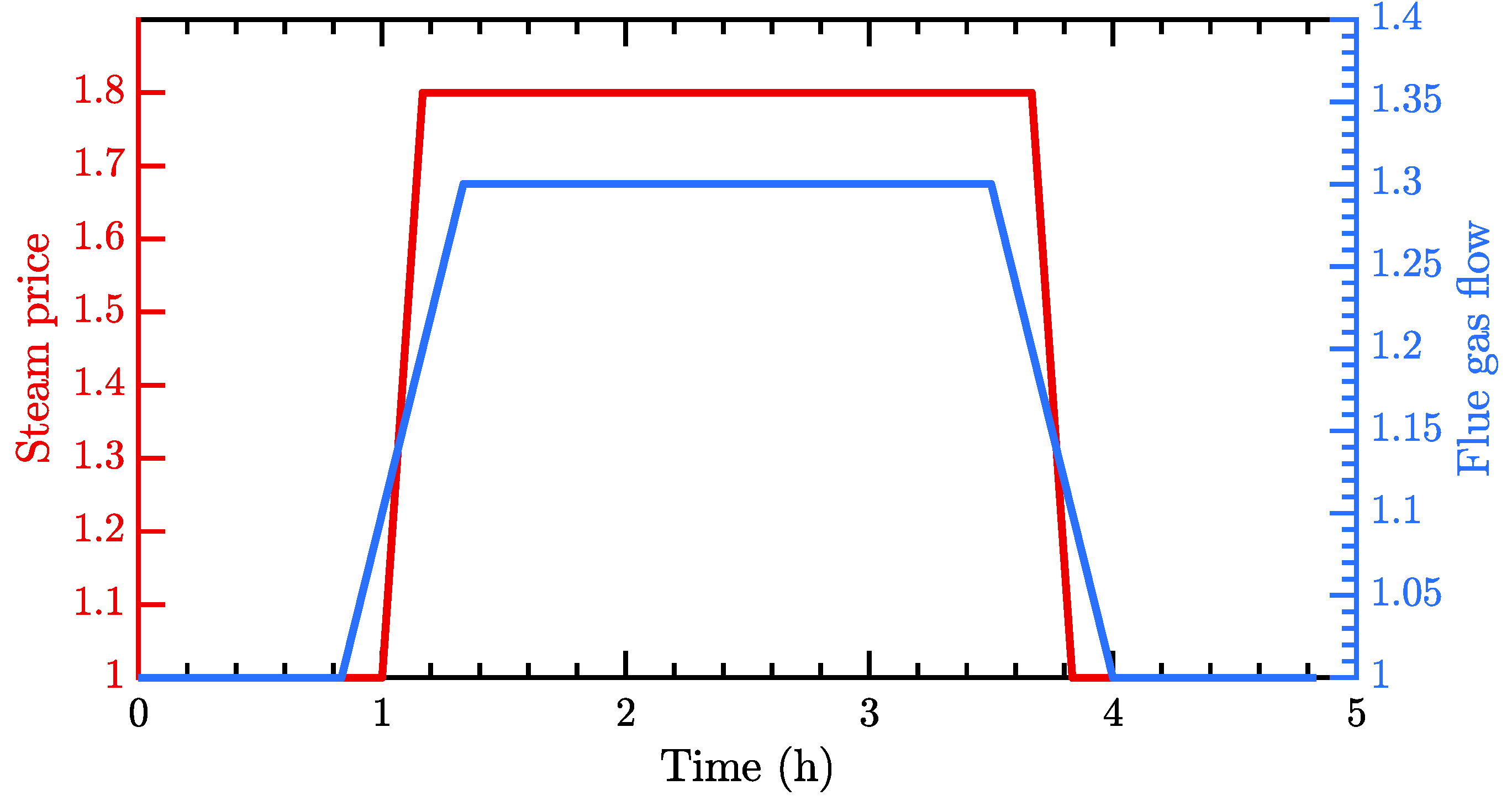
4.1.1. Time-Varying Steam Price and Flue Gas Flow Rate

In a typical power plant, the operation is periodic everyday (24 h). The demand for electricity is usually low at dawn and rises to a peak in the middle of the day and then drops to a low at night. A consequence of changing electricity demand is that the flue gas flow rate fluctuates in a similar manner affecting the operation of the attached post combustion capture plant. Again, during the high peak periods, steam, which is required in the regeneration section, may be unavailable since it will be needed for electricity generation. It is therefore important to determine how a deployed controller in the PCC plant reacts to such changes. The selected MPC controller was compared to EMPC in terms of economic performance. To assess the performance of EMPC and MPC for this kind of operation, the 24-h operation was scaled to 5 h. Figure 3 shows the shape of a periodic disturbance for both the steam price and the flue gas flow rate. The demand for electricity is low in the first hour which translates into a low flue gas flow rate. It then ramps up for half an hour and remains constant for 2 h before ramping down. In addition, as the demand for electricity increases, a decision has to be made whether to use the steam to generate more electricity or channel it to the PCC plant for CO${}_2$ regeneration. This decision is accounted for as an increase in the price of steam. The nominal value for the price of steam was taken from the study of He et al. [9].

4.1.2. Tracking MPC Parameter Tuning

To ensure fair comparison of the two controllers, the MPC need to be well tuned. Several MPC tuning techniques exist. However, in this work, the MPC was tuned such that the closed-loop trajectories and economic performance of MPC was as close as possible to that of EMPC. This was achieved using two step tests. The first step test corresponds to a state where the plant transitions from a peak electricity demand period (steam price is 1.8 and flue gas flow is 1.3) to a low electricity demand period (steam price is 1.0 and flue gas flow is 1.0). The second step test is the reverse of the first step test where the plant transitions from a low electricity demand period to a peak electricity demand period. Three MPCs with different tuning parameters (as shown in

Table 2. Tuning parameters for the three different MPCs tested. MPC: Model Predictive Control.

MPC	a	b	c	d
I	0.0001	0.01	0	0
II	0.0001	0.01	0.05	0.05
III	1.0	0.01	0.05	0.05

) and EMPC were designed and tested on the step tests. The resulting closed-loop trajectories are shown in Figure 4 and Figure 5.

Based on Figure 4 and Figure 5, MPC II was chosen for further tests. The weighting matrices are shown below. These parameters imply weakly tracking the CO${}_2$ emission as compared to the reboiler temperature and putting less weights on the inputs. The weights on the inputs are to ensure that the MPC does not make excessive control actions as compared to that of the EMPC:

$$Q=\left[\begin{array}{cc}a& 0\\ 0& b\end{array}\right],R=\left[\begin{array}{cc}c& 0\\ 0& d\end{array}\right]$$

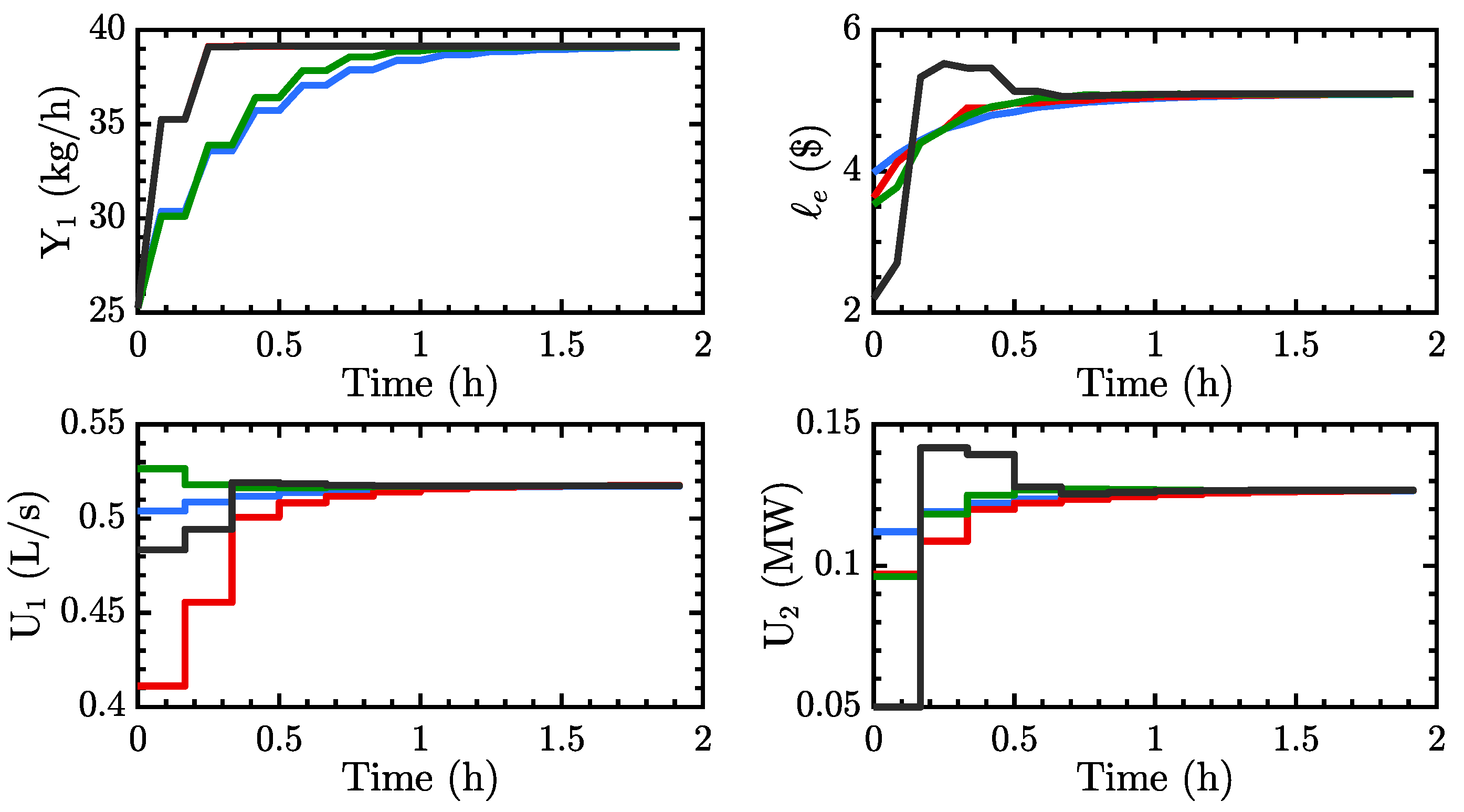
4.2. MPC Set-Point Update Strategy

In this work, the set-point update strategy is based on the frequency at which the steady-state optimization (SSO) of is carried out. Thus, the optimal steady-state operating point or set-point is determined at regular time intervals taking into consideration all information affecting the plant.

Table 3. Different MPC set-point update strategies and percent decrease in economics and heat duty. Heat duty is defined as the ratio of the amount of reboiler heat input to the mass of CO${}_2$ absorbed.

Strategy	Description	Avg. Cost (%)	Avg. Heat Duty (%)
1	No update/Fixed operating point	5.83	6.52
2	Update every hour	2.02	4.27
3	Update every 30 min	0.79	2.99
4	Update every 10 min (sampling time)	0.03	2.32

shows different MPC set-point update strategies, and their impact on the economic performance and heat duty compared to that of EMPC. For example, in strategy 1, the set-point is kept constant throughout the operation of the plant irrespective of the changes in flue gas flow rate and price of steam. In strategies 2–4, on the other hand, the SSO is computed and the set-point of MPC is updated at regular time intervals according to the update frequency. It can be observed in Table 3 that not updating the set-point is the worst strategy economically. This is because, when the set-point is kept constant throughout the operation of the PCC plant, any fluctuation in the flue gas flow rate is rejected at the expense of high operating costs. This is shown in Figure 6. This gets better as the frequency of the updates increase. Updating the set-point every sampling time (10 min) is the best option, however, it still leaves an economic and heat duty gap between MPC and EMPC. This could be because the SSO layer does not take into account future economic information resulting in some economic losses and ineffective use of steam for regeneration.

4.3. Operation under Different Carbon Tax Policies

In this set of simulations, the two operating scenarios are considered. In the first scenario, a tax-free emission limit is imposed. Emission beyond this limit leads to economic penalties. In the second scenario, charges are applied to any CO${}_2$ emitted. These scenarios were implemented as soft constraints in Optimization problems 1 and 3. Considering the scale of the PCC plant used in this study, $y_{limit}$ in Equations (26) and (45) was fixed at a value of 10.00 $\mathrm{kg}/\mathrm{h}$ and 0.00 $\mathrm{kg}/\mathrm{h}$ for the first and second scenarios, respectively. The horizon (prediction and control) for both MPC and EMPC is fixed at 360 min with a sampling time of 10 min (this implies N = 36). An MPC-SSO structure is used with MPC set-point update frequency of 1 h. The weighting matrices of the MPC are the same as the ones presented in Section 4.1. All information (flue gas flow rate and price of steam) is available to both controllers. In the case of MPC, the SSO uses the instantaneous information on the flue gas flow rate and the steam price to conduct steady-state economic optimization and updates the set-point of MPC every hour while in the case of EMPC, future information is used to determine the optimal input to the PCC plant at every sampling time. The MPC uses future information on the flue gas flow rate to determine the optimal input to the PCC plant to reach the target set-point every sampling time. The simulation time is 5 h with time-varying steam price and flue gas flow rate as presented in Figure 3.

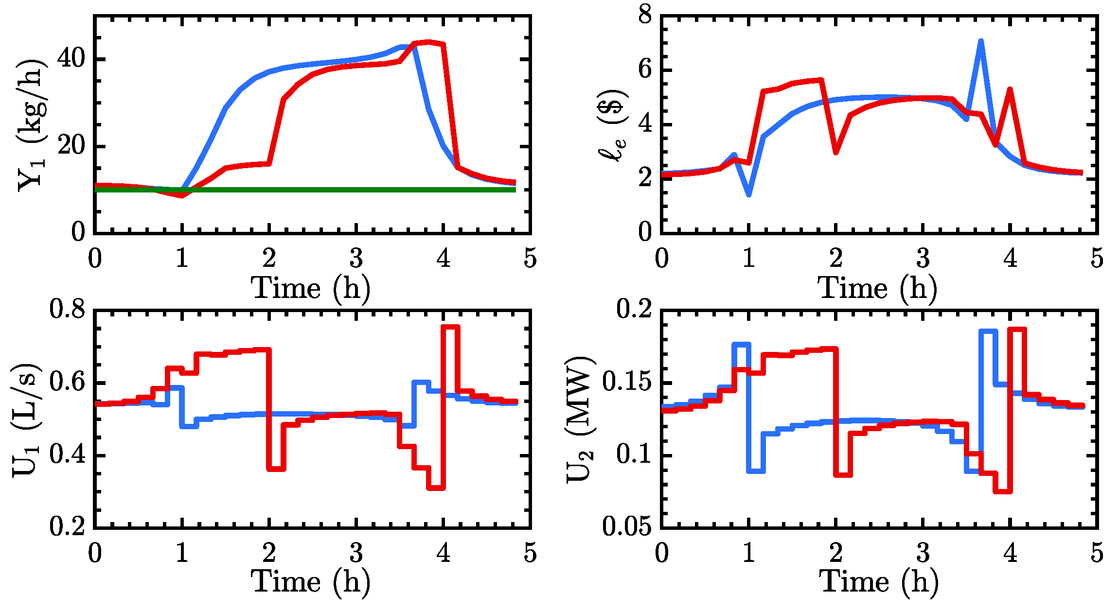
4.3.1. Carbon Tax with Tax-Free Emission Limit

Four sets of simulations are conducted in this scenario. The settings remained the same in each of the simulations with the exception of the carbon tax, which varied from simulation to simulation. The carbon tax considered are $50.00, $100.00, $150.00 and $200.00 per tonne CO${}_2$. The goal is to determine the operating strategy, compare the economic performance and the influence of the carbon tax on the performance of the two controllers under scenario one.

Figure 7 and Figure 8 show the CO${}_2$ emission, input and economic cost trajectories for the PCC process for each controller under scenario one at carbon tax of $50.00 and $200.00, respectively. At a carbon tax of $50.00 per tonne CO${}_2$ (Figure 7), both EMPC and MPC-SSO schemes either stayed on or above the emission limit. This is because there is no incentive for capturing more CO${}_2$ and operating below the emission limit. In addition, the effect of not considering the process economics every sampling time for MPC can be seen in the CO${}_2$ emission trajectories of the system. EMPC starts to quickly violate the emission limit as a result of the increase in flue gas flow rate and heat price while MPC sluggishly does that. The sluggishness could be because MPC tries to reject the ramp change in the flue gas flow rate until the set-point is updated by the SSO. Again, in the last hour when the flue gas flow rate and heat price decrease, EMPC rapidly decreases the emissions compared to that of MPC. Although MPC had information about the ramp increase and decrease in flue gas flow rate, it had no idea of the change in steam price, hence the sluggishness. This information became available to MPC only after the set-point of MPC was updated by the SSO. However, in the case of EMPC, both heat price and flue gas flow rate were considered. Again, in Figure 8, both controllers tried to stay above the emission limit—however, with much less emissions compared to when the carbon tax is $50.00 per tonne CO${}_2$. This is because there is much more weight now on emissions compared to the cost of steam. It can also be observed that the CO${}_2$ emission trajectories of both MPC and EMPC are different. MPC operates well below the emission limit and uses much more resources without any economic gains. Another reason is that, at a carbon tax of $200.00, the control dynamics change from slow tracking of CO${}_2$ to fast tracking. However, MPC had already been tuned for a single case and needed re-tuning. This resulted in the increase in both the average economic cost and heat duty (Figure 9 and Figure 10).

The average economic performances and heat duties of MPC and EMPC under scenario one and different carbon tax is shown in Figure 9 and Figure 10. As can be observed in Figure 9, the economic performance gap between MPC and EMPC remained fairly constant as the carbon tax increases until $150.00, where the gap widened. Similarly, the gap between the average heat duty remained the same until $150.00 where it increases. One possible explanation for this is that, in this scenario, when the PCC plant operates on the emission limit, the carbon tax is not charged. Only the heat input is optimized. The dynamics of the economics therefore changes from heat input to CO${}_2$ emissions and back to heat input. This shifting dynamics could have resulted in the increased gap between MPC and EMPC when the CO${}_2$ price is high. In addition, one key observation is that the gap between MPC and EMPC is smaller for the economic cost compared to the heat duty plot. This implies that though the economics seem to be close, the heat input is not efficiently used in the case of MPC compared to EMPC. Thus, to ensure a better economic performance and heat duty of MPC, re-tuning or increased update frequency is probably necessary. However, determining the optimal tuning parameters of MPC is not always obvious and is a major challenge in MPC design. EMPC on the other hand is able to determine the optimal operating strategy without requiring an update in the controller settings and change in set-point update strategy. This makes EMPC well suited for flexible operation of the PCC process while being energy efficient.

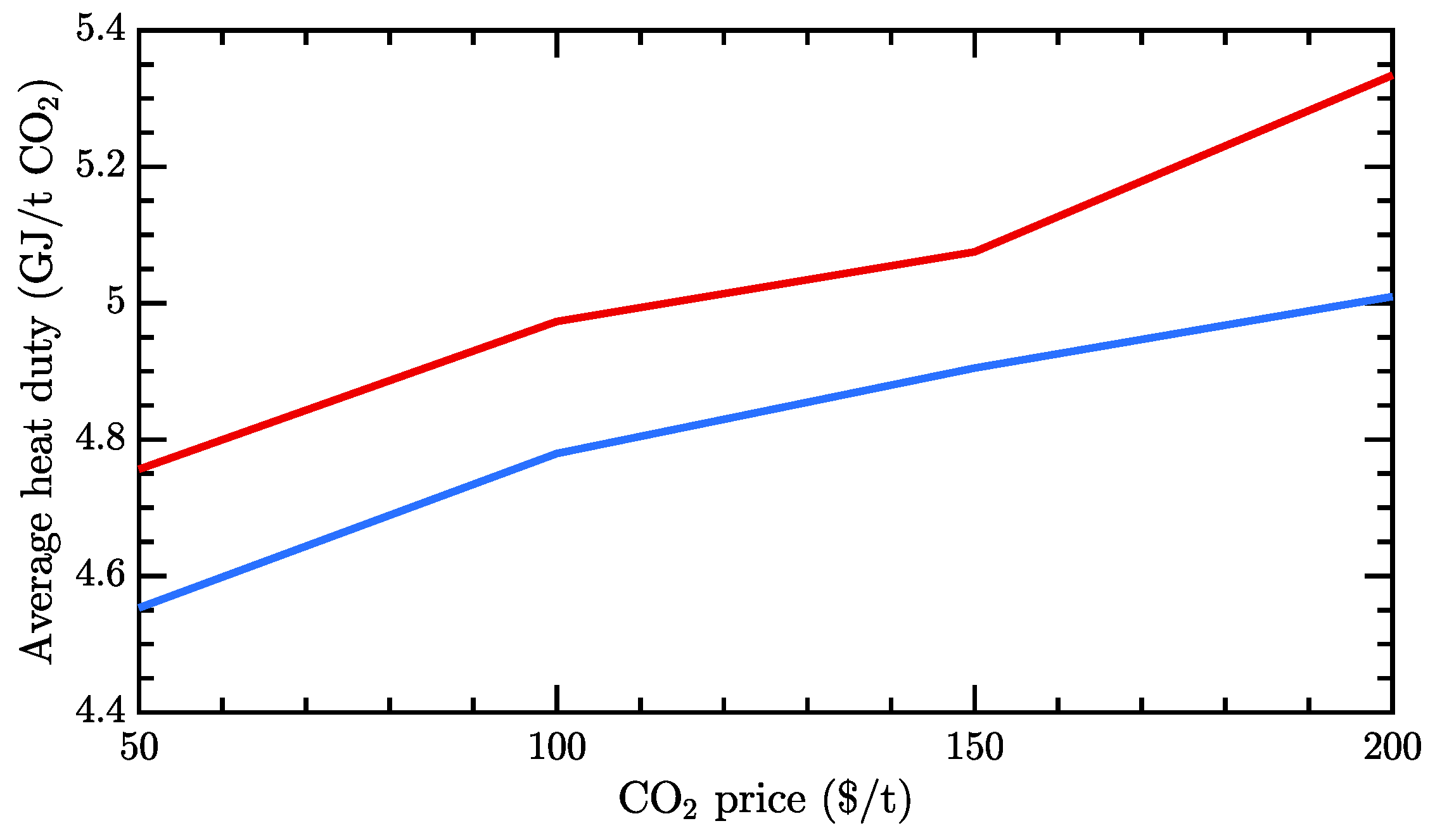
4.3.2. Carbon Tax without Tax-Free Emission Limit

The simulations conducted in this section and their purpose is similar to that of scenario one. The controller settings therefore remain the same. The only difference between the two scenarios is how the carbon tax is enforced. In this scenario, charges are applied to any CO${}_2$ released into the atmosphere. In Figure 11 and Figure 12, the CO${}_2$ emission trajectory for both controllers remain fairly the same in the first three hours and begin to differ slightly in the last two hours. However, this difference is not significant enough to cause much differences in the performance metrics (economic cost and heat duty) when the carbon tax increases. This can be observed in Figure 13 and Figure 14 where the gaps in the average economic cost and average heat duty are almost constant. Similar to the results in scenario one, the gap in the heat duty between MPC and EMPC is wider compared to their economic performance. Thus, under this scenario, changes in the carbon tax does not affect the performance of the controllers. This could be because, throughout the operation, the cost of CO${}_2$ emission dominates the decision making as compared to the case of scenario one where, when the PCC plant operates on the emission limit, CO${}_2$ emissions are not penalized. The difference in economic performance of both controllers can therefore be solely attributed to the timescale separation between MPC and SSO.

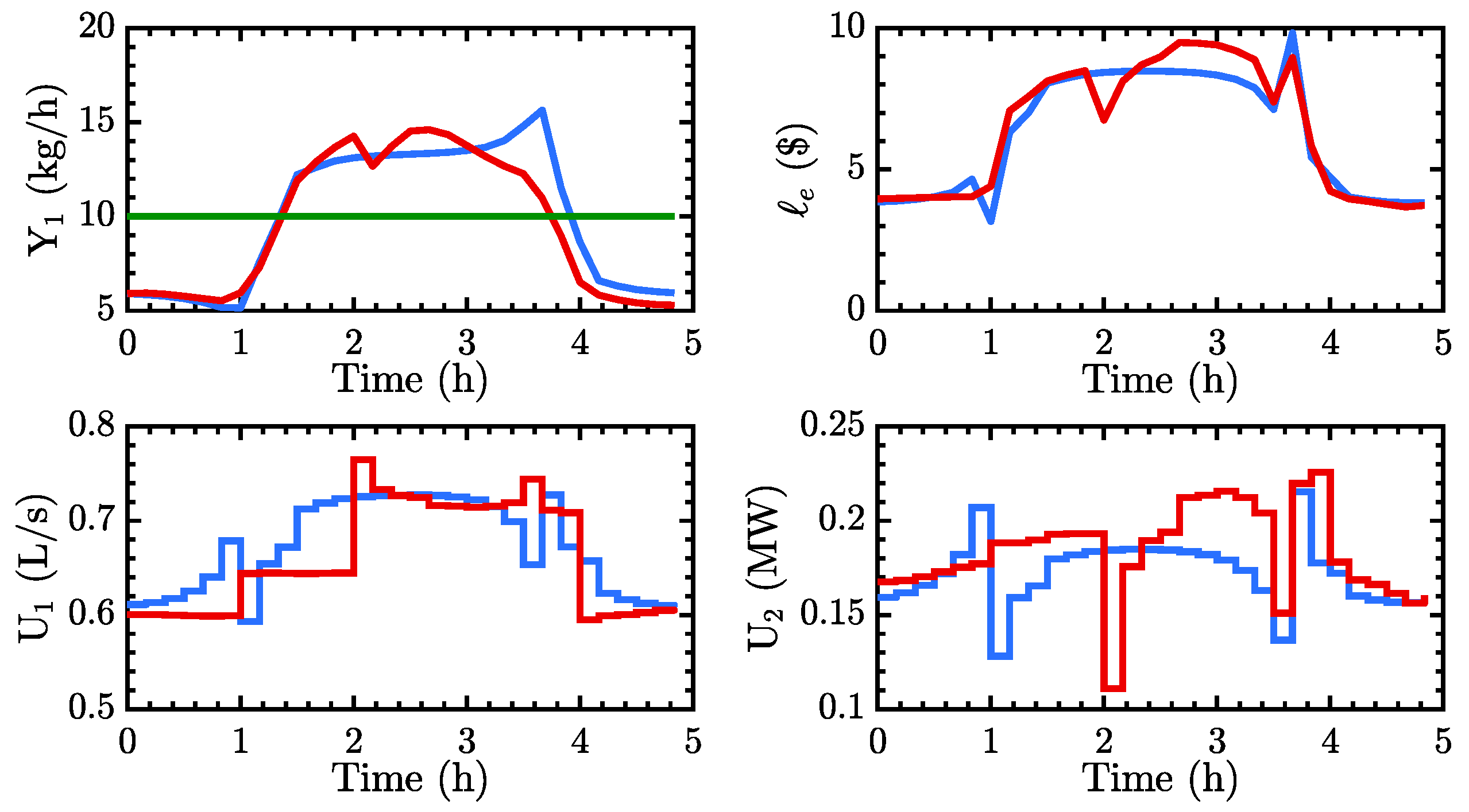
4.4. Operation under Uncertainty

The presence of disturbances is a problem in many practical MPC applications. This could result in performance degradation or infeasibility. In this section, we subject the PCC process to disturbances in the flue gas flow rate and CO${}_2$ concentration. This is to test the susceptibility of the controllers to uncertainties. The uncertainties were obtained by adding Gaussian white noise to the flue gas flow rate and flue gas concentration, respectively. The simulation for each uncertainty was repeated many times, each time with a different random number seed value (varied from 1 to 10). Only one of plots for each uncertainty experiment has been presented. The controller design for both MPC and EMPC remain the same as the previous sections.

Figure 15 and Figure 16 show the trajectories of CO${}_2$ emission, economic cost and inputs for both controllers under uncertainty in flue gas flow rate and CO${}_2$ concentration, respectively. As can be observed in the figures, both controllers showed the satisfactory performance with very little performance degradation. Thus, under small uncertain disturbances, both controllers perform the same when there is uncertainty in the flue gas flow rate and concentration. One reason for this observation could be that the PCC plant is insensitive to small disturbances. However, due to numerical challenges encountered at high disturbances, further tests were not conducted. Uncertainty in the steam price was not considered because it is only considered in the cost function and does not affect the process dynamics. Thus, both controllers are expected to be affected in the same way.

5. Conclusions

Attaching an amine-based PCC plant to a power plant reduces the overall efficiency of the power plant especially in the wake of frequent changes in electricity demand and diversification of electricity generation sources. However, operating the PCC plant in a flexible manner can reduce the impact of attaching a PCC plant to a power plant. This study investigates the operation of a PCC process under time-varying disturbances in flue gas flow rate and steam price using EMPC. The economic cost and heat duty of the operation of the PCC process under EMPC was compared to that of tracking MPC. Two scenarios, namely with and without emission limits, were also investigated. This was achieved by first presenting a first principle model of the PCC process—followed by formulation and design of both controllers and the solution to the resulting optimization problems using the simultaneous approach for dynamic optimization.

The results show that operating the PCC plant at a constant set-point leads to significant economic losses and inefficient utilization of the steam from the power plant. Specifically, operating the PCC plant in a time-varying fashion using EMPC improves the operation of the process up to about 6% in terms of economic efficiency and 7% in terms of heat duty or energy efficiency. In addition, a nearly constant gap between the average economic cost and heat duty of the process operation at different carbon prices using EMPC and MPC was observed with the heat duty having a larger gap compared to the economic cost. However, under scenario one, the gap further increased at a CO${}_2$ price of $200.00 per tonne, whereas the gap remained fairly the same under scenario two. Although this gap can be reduced by increasing the frequency of updating the set-point of MPC and/or re-tuning MPC altogether, obtaining the optimal tuning parameters of MPC is not always obvious. EMPC, on the other hand, was able to determine the appropriate control policy depending on the scenario without further tuning or updating. This makes it suitable for flexible operation of the PCC process while being energy efficient. Finally, it was observed in this study that both controllers are robust to small uncertain disturbances in the flue gas flow rate and concentration. The insight gained from this study is useful in an era where our energy demands need to be met while ensuring that emissions are at a minimum.

References

1. Miller, B.G. Fossil Fuel Emission Control Technologies: Stationary Heat and Power Systems, 1st ed.; Elsevier: Waltham, MA, USA, 2015. [Google Scholar]
2. Metz, B.; Intergovernmental Panel on Climate Change (Eds.) IPCC Special Report on Carbon Dioxide Capture and Storage; Cambridge University Press: Cambridge, UK, 2005. [Google Scholar]
3. Davison, J.; Mancuso, L.; Ferrari, N. Costs of CO2 Capture Technologies in Coal Fired Power and Hydrogen Plants. Energy Procedia 2014, 63, 7598–7607. [Google Scholar] [CrossRef]
4. Ziaii, S.; Rochelle, G.T.; Edgar, T.F. Dynamic Modeling to Minimize Energy Use for CO2 Capture in Power Plants by Aqueous Monoethanolamine. Ind. Eng. Chem. Res. 2009, 48, 6105–6111. [Google Scholar] [CrossRef]
5. Lin, Y.J.; Wong, D.S.H.; Jang, S.S.; Ou, J.J. Control Strategies for Flexible Operation of Power Plant with CO2 Capture Plant. AIChE J. 2012, 58, 2697–2704. [Google Scholar] [CrossRef]
6. Bedelbayev, A.; Greer, T.; Lie, B. Model Based Control of Absorption Tower for CO2 Capturing. In Proceedings of the 49th International Conference of Scandinavian Simulation Society (SIMS 2008), Oslo, Norway, 7–8 October 2008. [Google Scholar]
7. Panahi, M.; Skogestad, S. Economically Efficient Operation of CO2 Capturing Process Part I: Self-Optimizing Procedure for Selecting the Best Controlled Variables. Chem. Eng. Process. 2011, 50, 247–253. [Google Scholar] [CrossRef]
8. Panahi, M.; Skogestad, S. Economically Efficient Operation of CO2 Capturing Process. Part II. Design of Control Layer. Chem. Eng. Process. 2012, 52, 112–124. [Google Scholar] [CrossRef]
9. He, Z.; Sahraei, M.H.; Ricardez-Sandoval, L.A. Flexible Operation and Simultaneous Scheduling and Control of a CO2 Capture Plant Using Model Predictive Control. Int. J. Greenh. Gas Control 2016, 48, 300–311. [Google Scholar] [CrossRef]
10. Bankole, T.; Jones, D.; Bhattacharyya, D.; Turton, R.; Zitney, S.E. Optimal Scheduling and Its Lyapunov Stability for Advanced Load-Following Energy Plants with CO2 Capture. Comput. Chem. Eng. 2018, 109, 30–47. [Google Scholar] [CrossRef]
11. Mac Dowell, N.; Shah, N. The Multi-Period Optimisation of an Amine-Based CO2 Capture Process Integrated with a Super-Critical Coal-Fired Power Station for Flexible Operation. Comput. Chem. Eng. 2015, 74, 169–183. [Google Scholar] [CrossRef]
12. Ellis, M.; Durand, H.; Christofides, P.D. A Tutorial Review of Economic Model Predictive Control Methods. J. Process Control 2014, 24, 1156–1178. [Google Scholar] [CrossRef]
13. Angeli, D.; Amrit, R.; Rawlings, J.B. On Average Performance and Stability of Economic Model Predictive Control. IEEE Trans. Autom. Control 2012, 57, 1615–1626. [Google Scholar] [CrossRef] [Green Version]
14. Liu, S.; Liu, J. Economic Model Predictive Control with Extended Horizon. Automatica 2016, 73, 180–192. [Google Scholar] [CrossRef]
15. Zeng, J.; Liu, J. Economic Model Predictive Control of Wastewater Treatment Processes. Ind. Eng. Chem. Res. 2015, 54, 5710–5721. [Google Scholar] [CrossRef]
16. Liu, S.; Zhang, J.; Liu, J. Economic MPC with Terminal Cost and Application to an Oilsand Primary Separation Vessel. Chem. Eng. Sci. 2015, 136, 27–37. [Google Scholar] [CrossRef]
17. Idris, E.A.; Engell, S. Economics-Based NMPC Strategies for the Operation and Control of a Continuous Catalytic Distillation Process. J. Process Control 2012, 22, 1832–1843. [Google Scholar] [CrossRef]
18. Mendoza-Serrano, D.I.; Chmielewski, D.J. Smart Grid Coordination in Building HVAC Systems: EMPC and the Impact of Forecasting. J. Process Control 2014, 24, 1301–1310. [Google Scholar] [CrossRef]
19. Touretzky, C.R.; Baldea, M. Integrating Scheduling and Control for Economic MPC of Buildings with Energy Storage. J. Process Control 2014, 24, 1292–1300. [Google Scholar] [CrossRef]
20. Harun, N.; Nittaya, T.; Douglas, P.L.; Croiset, E.; Ricardez-Sandoval, L.A. Dynamic Simulation of MEA Absorption Process for CO2 Capture from Power Plants. Int. J. Greenh. Gas Control 2012, 10, 295–309. [Google Scholar] [CrossRef]
21. Whitman, W.G. The Two Film Theory of Gas Absorption. Int. J. Heat Mass Trans. 1962, 5, 429–433. [Google Scholar] [CrossRef]
22. Onda, K.; Takeuchi, H.; Okumoto, Y. Mass Transfer Coefficients between Gas and Liquid Phases in Packed Columns. J. Chem. Eng. Jpn. 1968, 1, 56–62. [Google Scholar] [CrossRef]
23. Danckwerts, P. The Reaction of CO2 with Ethanolamines. Chem. Eng. Sci. 1979, 34, 443–446. [Google Scholar] [CrossRef]
24. Tobiesen, F.A.; Juliussen, O.; Svendsen, H.F. Experimental Validation of a Rigorous Desorber Model for CO2 Post-Combustion Capture. Chem. Eng. Sci. 2008, 63, 2641–2656. [Google Scholar] [CrossRef]
25. Chilton, T.H.; Colburn, A.P. Mass Transfer (Absorption) Coefficients Prediction from Data on Heat Transfer and Fluid Friction. Ind. Eng. Chem. 1934, 26, 1183–1187. [Google Scholar] [CrossRef]
26. Harun, N. Dynamic Simulation of MEA Absorption Process for CO2 Capture from Power Plants. Ph.D. Thesis, University of Waterloo, Waterloo, ON, USA, 2012. [Google Scholar]
27. Amrit, R.; Rawlings, J.B.; Biegler, L.T. Optimizing Process Economics Online Using Model Predictive Control. Comput. Chem. Eng. 2013, 58, 334–343. [Google Scholar] [CrossRef]
28. Biegler, L.T. Nonlinear Programming: Concepts, Algorithms, and Applications to Chemical Processes; Society for Industrial and Applied Mathematics: Philadelphia, PA, USA, 2010. [Google Scholar]
29. Andersson, J.A.E.; Gillis, J.; Horn, G.; Rawlings, J.B.; Diehl, M. CasADi—ASoftware Framework for Nonlinear Optimization and Optimal Control. Math. Program. Comput. 2018. [Google Scholar] [CrossRef]
30. Wächter, A.; Biegler, L.T. On the Implementation of an Interior-Point Filter Line-Search Algorithm for Large-Scale Nonlinear Programming. Math. Program. 2006, 106, 25–57. [Google Scholar] [CrossRef]
Figure 1. Overview of electricity generation with post-combustion CO 2 capture.
Processes 06 00135 g001
Figure 2. Schematic diagram of a full cycle amine-based post-combustion capture plant.
Processes 06 00135 g002
Figure 3. Scaled hourly changes in steam price (Nominal value: $0.01 / kg ) and flue gas flow rate (Nominal value: 0.0832 m 3 / s ). Price (red), Flue gas flow (blue).
Processes 06 00135 g003
Figure 4. Closed-loop trajectories of EMPC and different MPC tuning parameters starting from a higher economic cost to a lower one. EMPC (blue), MPC I (red), MPC II (green), MPC III (black). The average economic performances are 4.700, 4.768, 4.713, 4.692 for EMPC, MPC I, MPC II, MPC III, respectively; (top-left) mass flow rate of CO 2 in the treated flue gas; (top-right) economic performance of controller; (bottom-left) volumetric flow rate of solvent; (bottom-right) heat input to reboiler. EMPC: Economic Model Predictive Control
Processes 06 00135 g004
Figure 5. Closed-loop trajectories of EMPC and different MPC tuning parameters starting from a lower economic cost to a higher one. EMPC (blue), MPC I (red), MPC II (green), MPC III (black). The average economic performances are 3.654, 3.668, 3.650, 3.685 for EMPC, MPC I, MPC II, MPC III, respectively; (top-left) mass flow rate of CO 2 in the treated flue gas; (top-right) economic performance of controller; (bottom-left) volumetric flow rate of solvent; (bottom-right) heat input to reboiler.
Processes 06 00135 g005
Figure 6. CO 2 emission, input and economic cost trajectories of the PCC plant with carbon tax set at $50.00 per tonne CO 2 . The set-point of MPC is not updated. EMPC (blue), MPC (red), Emission limit (green); (top-left) mass flow rate of CO 2 in the treated flue gas; (top-right) economic performance of controller; (bottom-left) volumetric flow rate of solvent; (bottom-right) heat input to reboiler. PCC: Post-combustion CO 2 Capture.
Processes 06 00135 g006
Figure 7. CO 2 emission, input and economic cost trajectories of the PCC plant for scenario 1 with carbon tax set at $50.00 per tonne CO 2 . EMPC (blue), MPC (red), Emission limit (green); (top-left) mass flow rate of CO 2 in the treated flue gas; (top-right) economic performance of controller; (bottom-left) volumetric flow rate of solvent; (bottom-right) heat input to reboiler.
Processes 06 00135 g007
Figure 8. CO 2 emission, input and economic cost trajectories of the PCC plant for scenario 1 with carbon tax set at $200.00 per tonne CO 2 . EMPC (blue), MPC (red), Emission limit (green); (top-left) mass flow rate of CO 2 in the treated flue gas; (top-right) economic performance of controller; (bottom-left) volumetric flow rate of solvent; (bottom-right) heat input to reboiler.
Processes 06 00135 g008
Figure 9. Average economic performance of the controllers under scenario 1 at different CO 2 prices. EMPC (blue), MPC (red).
Processes 06 00135 g009
Figure 10. Average heat duty of the controllers under scenario 1 at different CO 2 prices. EMPC (blue), MPC (red).
Processes 06 00135 g010
Figure 11. CO 2 emission, input and economic cost trajectories of the PCC plant for scenario 2 with carbon tax set at $50.00 per tonne CO 2 . EMPC (blue), MPC (red), Emission limit (green); (top-left) mass flow rate of CO 2 in the treated flue gas; (top-right) economic performance of controller; (bottom-left) volumetric flow rate of solvent; (bottom-right) heat input to reboiler.
Processes 06 00135 g011
Figure 12. CO 2 emission, input and economic cost trajectories of the PCC plant for scenario 2 with carbon tax set at $200.00 per tonne CO 2 . EMPC (blue), MPC (red), Emission limit (green); (top-left) mass flow rate of CO 2 in the treated flue gas; (top-right) economic performance of controller; (bottom-left) volumetric flow rate of solvent; (bottom-right) heat input to reboiler.
Processes 06 00135 g012
Figure 13. Average economic performance of the controllers under scenario 2 at different CO 2 prices. EMPC (blue), MPC (red).
Processes 06 00135 g013
Figure 14. Average heat duty of the controllers under scenario 2 at different CO 2 prices. EMPC (blue), MPC (red).
Processes 06 00135 g014
Figure 15. CO 2 emission, inputs and economic cost trajectories of the PCC plant under uncertainty in flue gas flow rate. Nominal value =1.0. Uncertainty generated by adding Gaussian white noise with zero mean and standard deviation σ = 0.1, to the flue gas flow rate. EMPC (blue), MPC (red); (top-left) mass flow rate of CO 2 in the treated flue gas; (top-right) economic performance of controller; (bottom-left) volumetric flow rate of solvent; (bottom-right) heat input to reboiler.
Processes 06 00135 g015
Figure 16. CO 2 emission, inputs and economic cost trajectories of the PCC plant under uncertainty in flue gas CO 2 concentration. Uncertainty generated by adding Gaussian white noise with zero mean and standard deviation σ = 0.06, to the flue gas CO 2 concentration. EMPC (blue), MPC (red); (top-left) mass flow rate of CO 2 in the treated flue gas; (top-right) economic performance of controller; (bottom-left) volumetric flow rate of solvent; (bottom-right) heat input to reboiler.
Processes 06 00135 g016