Article

Individual-Based Modelling of Invasion in Bioaugmented Sand Filter Communities

1
KERMIT, Department of Data Analysis and Mathematical Modelling, Ghent University, Coupure links 653, B-9000 Ghent, Belgium
2
Division of Soil and Water Management, KU Leuven, Kasteelpark Arenberg 20 bus 2459, B-3001 Heverlee, Belgium
3
Center for Microbial Ecology and Technology (CMET), Ghent University, Coupure links 653, B-9000 Ghent, Belgium
*
Author to whom correspondence should be addressed.
Processes 2018, 6(1), 2; https://doi.org/10.3390/pr6010002
Submission received: 28 August 2017 / Revised: 24 October 2017 / Accepted: 30 October 2017 / Published: 1 January 2018

Abstract

:
Using experimental data obtained from in vitro bioaugmentation studies of a sand filter community of 13 bacterial species, we develop an individual-based model representing the in silico counterpart of this synthetic microbial community. We assess the inter-species interactions, first by identifying strain identity effects in the data then by synthesizing these effects into a competition structure for our model. Pairwise competition outcomes are determined based on interaction effects in terms of functionality. We also consider non-deterministic competition, where winning probabilities are assigned based on the relative intrinsic competitiveness of each strain. Our model is able to reproduce the key qualitative dynamics observed in in vitro experiments with similar synthetic sand filter communities. Simulation outcomes can be explained based on the underlying competition structures and the resulting spatial dynamics. Our results highlight the importance of community diversity and in particular evenness in stabilizing the community dynamics, allowing us to study the establishment and development of these communities, and thereby illustrate the potential of the individual-based modelling approach for addressing microbial ecological theories related to synthetic communities.

1. Introduction

1.1. Background

The composition, establishment and functional maintenance of any ecosystem are largely driven by the interactions between individuals [1], and microbial communities are no exception [2]. The fundamental basis of all studies of interactions between cell populations are synthetic co-culture systems: experimental set-ups where “two or more different populations of cells are grown with some degree of contact between them” [3]. Synthetic co-cultures have gained particular interest from microbiologists in recent years due to their reduced complexity and increased controllability, which favours them over more complex natural systems for examining ecological theories [4] and also for more specific industrial, medical and environmental applications such as industrial fermentation and the production of chemical compounds [5].
A more specific application of co-cultures is bioaugmentation, where the biomass in soil or water treatment plants is altered by the addition of certain microbial strains that have been selected for their ability to degrade specific chemical compounds [6]. From a microbial ecological perspective, bioaugmentation represents a kind of microbial invasion process, where the strains introduced to augment resident community functionality are the invaders. For example, during the treatment of drinking water, the common groundwater pollutant 2,6-dichlorobenzamide (2,6-BAM) must be removed below a threshold concentration of 0.1 μ g / L to meet the EU Directive on Drinking Water [7]. However, the endogenous microbial communities in the sand filters (SFs) of such drinking water treatment plants are not capable of achieving sufficient BAM removal to respect this threshold [8]. Therefore, bioaugmentation of SFs has been proposed as an alternative strategy, by the addition of a specialized BAM mineralizer such as Aminobacter sp. MSH1 [9]. However, studies of this type of bioaugmentation of drinking water ecosystems rarely address how exactly the pesticide degrader interacts with the resident community, and other such fundamental ecological questions [10].
In Vandermaesen et al. [11], the authors hypothesize that the establishment of MSH1 and its subsequent BAM mineralization in SFs depend not only on exploitative competition effects, but also on other features such as interactions with resident community members. Therefore, the BAM mineralization activity of MSH1 was evaluated in sand microcosms in the presence of a selection of the 13 sand filter isolates (SFIs) described in Vandermaesen et al. [11]. Synthetic microbial communities of MSH1 combined with SFIs were subjected to an initial competition phase. Subsequently, BAM was added and the kinetics of BAM mineralization was evaluated as a measure of bioaugmentation success.
To characterize the interactions between resident community members, co-cultures of various combinations of SFIs with MSH1 were inoculated, and their mineralization kinetics was followed. However, given the total number of strains in the community, it is practically impossible to experimentally study all possible co-culture combinations. In such cases, mathematical modelling is becoming more and more appreciated as a tool for identifying possible co-cultures of interest [12,13,14,15].

1.2. Motivation and Scope

We use an individual-based modelling approach to construct the in silico counterpart of the in vitro synthetic community used in the experiments of Vandermaesen et al. [11], with the goal of qualitatively reproducing the observed dynamics. Due to their inherent flexibility and ability to reproduce complex system-level behaviour by capturing the interactions between individuals, individual-based models (IBMs) have proven useful for addressing fundamental microbial ecology questions, such as our questions related to fundamental interactions between invader and resident community members. Other examples include IBM studies of the evolution of cooperative behaviour in microbial communities [16] and the role of spatial aggregation in maintaining cooperation between cross-feeding microbial strains [17]. However, such models are typically restricted to only a few species, hence our model of 13 species would be an outlier in this respect [4].
Previous results with synthetic microbial communities with similar characteristics in terms of diversity and composition [18] and also for this particular synthetic community of MSH1 and 13 SFIs [11], highlighted the importance of the initial competition phase (before the addition of BAM) where all 13 SFIs are inoculated in the co-culture. Competition between the SFIs results in extinctions, leading to a stable subcommunity of reduced richness. It is this subcommunity that is present at the moment of the BAM spike and during the subsequent mineralization period that determines the bioaugmentation success. We aim to retrieve this behaviour with our modelling approach.
For this purpose, we make use of the data obtained from the Vandermaesen et al. experiments [11] (described in Section 2) to model the competitive interactions between individual microbes. We then present the results of inferring the strain interactions (Section 3.1), incorporating this information in an IBM (Section 3.2), as well as the results of the in silico experiments it is subsequently employed for (Section 3.3). In the final section, we summarize the conclusions of the modelling and simulation studies.

2. Materials and Methods

In this section, we summarize the experimental set-up and procedure used by Vandermaesen et al. [11] to obtain the dataset used for the modelling and simulation studies presented in this paper.

2.1. Experimental Set-Up

The hypothesis of this in vitro study was that the establishment of MSH1 and its subsequent BAM mineralization in SFs depend on interactions with and between resident community members. Therefore, the BAM mineralization activity of MSH1 was evaluated in sand microcosm co-cultures in the presence of different combinations of 13 SFIs. Synthetic microbial communities of MSH1 combined with SFIs were co-cultured, then BAM was added and the kinetics of BAM mineralization was evaluated as a measure of bioaugmentation success.

2.1.1. Bacterial Strains

The specific variant of the BAM mineralizing Aminobacter sp. MSH1 [9] used in this study, MSH1-GFP, was fluorescently tagged. The 13 SFIs used were isolated from SF material from two drinking water treatment plants [11]: Acidovorax sp. S9, Undibacterium sp. S22, Brachybacterium sp. S51, Mesorhizobium sp. S158, Acidovorax sp. S164, Rhodococcus sp. K27, Acidovorax sp. K52, Aeromonas sp. K62, Paucibacter sp. K67, Pelomonas sp. K89, Rhodoferax sp. K112, Rhodoferax sp. K129, and Piscinibacter sp. K169. None of the selected SFIs were capable of BAM mineralization, avoiding any confounding effects with the BAM mineralization performance of MSH1.

2.1.2. Microcosm Set-Up

Microcosms were created in deep 96-well plates, containing sterile sand in every well. MSH1 and SFIs were cultured and prepared as described in Vandermaesen et al. [11] and combined in synthetic communities in such a way that the number of cells of every strain was 107 cells/mL. Since each community included MSH1, the total richness of a community R T is given by R T = R SFI + 1, where R SFI is the number of SFIs present. In addition to all combinations of individual SFI with MSH1 (13 combinations at R SFI = 1), all 78 different pair combinations of two SFIs with MSH1 ( R SFI = 2) were tested.
Sodium acetate was provided as the only carbon source at a concentration of 150 μ g / L in MMO medium (MMO + Ac). Assuming that 50% of acetate-C is actually assimilated, this corresponds to an AOC (assimilable organic carbon) concentration of 22 μ g C / L , which is within the range of AOC values in drinking water ecosystems (20–100 μ g C / L ) [19]. Of every synthetic community, 100 μ L was inoculated in the sand microcosms. A reference microcosm inoculated with 100 μ L MSH1 at 107 cells/mL ( R SFI = 0) was included in every deep well plate. In addition, to account for abiotic 14 CO 2 production, one negative control ( R T = 0) was included, containing sand amended with 100 μ L MMO + Ac. All synthetic communities and controls were replicated four times. No 14 CO 2 production was observed in the abiotic control. The plates were sealed and incubated at 20 °C for 7 days.
After this initial competition phase, all wells were spiked with 5000 counts per minute 14 C-BAM, dissolved in 5 μ L MMO, which corresponds to a final BAM concentration of 150 μ g / L . BAM mineralization was then followed for approximately 130 h by trapping the produced 14 CO 2 with Ca(OH) 2 . Trapped 14 CO 2 radioactivity was quantified by digital autoradiography. The cumulative percentage 14 CO 2 was plotted relative to the total amount of 14 C added as a function of the incubation time, and hence cumulative mineralization curves were obtained.

2.2. Modelling of Mineralization Kinetics

To describe the kinetics of BAM mineralization, the modified Gompertz model [20] was used. This model is one of the most commonly used microbial growth models [21], and is given by
P = A exp exp μ e A λ c t + 1
where P (%) is the percentage mineralization at time t ( h ), A (%) is the total extent of mineralization after the exponential mineralization phase, λ (% h 1 ) is the lag time, c (% h 1 ) is the endogenous mineralization rate, and μ (% h 1 ) is the maximum mineralization rate constant. The modified Gompertz model differs from the standard Gompertz model [20] in that its parameters each have a biological meaning.
The Gompertz parameters of the cumulative mineralization curves were determined by least squares curve fitting, using the Trust-Region-Reflective algorithm [22,23], at a termination tolerance of 10−14 and allowing at most 2 × 10⁵ function evaluations and 3 × 10⁵ iterations. Initial parameter estimates were set at 30, 5, 0.1, and 2 for A, μ , c, and λ , respectively [24]. This was implemented using Matlab R2012b (Mathworks, Natick, MA, USA). All values of c were zero or close to, and were hence excluded.

2.3. Description of the Dataset

From the experimental set-up described in Section 2.1, we obtained a dataset representing 13 monocultures (the individual strains) and 78 co-cultures (the pair combinations). For each of these 91 conditions, we have two types of mineralization data. First, a cumulative BAM mineralization time series consisting of achieved mineralization values at 13 time points, from t = 0 h to t = 130 h. There are four biological replicates of each time series, except where some outliers were removed as indicated in Vandermaesen et al. [11]. In total, 21 out of 364 time series were removed. After removal of these outliers, no condition had less than three replicates. The second data type consists of the fitted Gompertz parameters λ , μ and A describing the mineralization kinetics, namely one set of parameters per time series.

3. Results and Discussion

3.1. Assessing Strain Interactions

The experiments of Vandermaesen et al. [
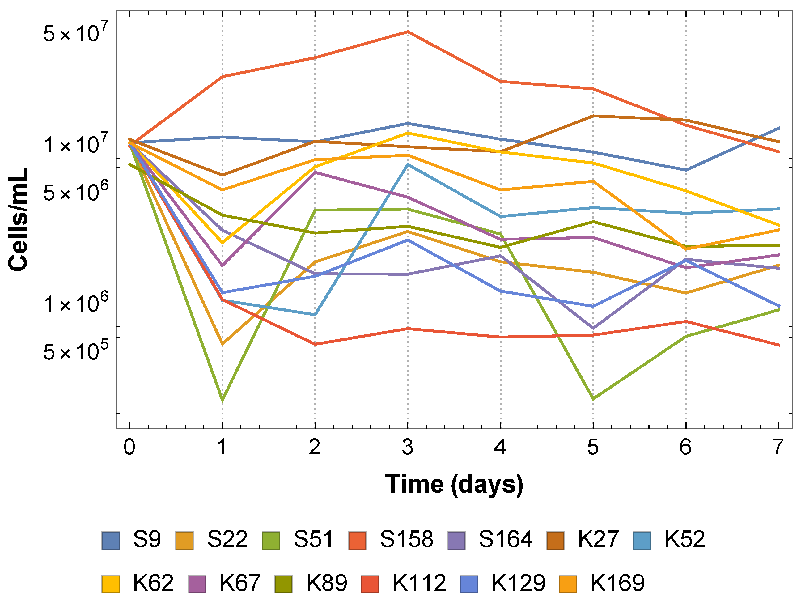
11] focused on bioaugmentation success and therefore collected data related to BAM mineralization and MSH1 survival. The data related to the SFIs themselves are their monoculture growth curves and their monoculture survival curves on acetate (see Appendix A). These data can give us an idea of how the SFIs grow and persist in isolation, and on this basis Vandermaesen et al. [11] classified the strains according to their “intrinsic competitiveness”, a classification that we can use as an additional feature of the strains. However, these data do not give us any information about how the SFIs may interact, and in particular compete, when they are inoculated together in co-culture.
The information we do have regarding the interactions between SFIs is indirect. From the differences in mineralization parameters between the different co-culture combinations, we can infer when there are interaction effects occurring between strains, by comparing the mineralization performances of MSH1 alone, in co-culture with individual SFIs, and in co-culture with both strains. The mineralization performance was studied using the Gompertz model (see Section 2.2 for details). This model has four parameters: the lag time λ , the maximum mineralization rate μ , the total extent of mineralization A, and the endogenous mineralization rate c.
To study the strain interaction effects, we focus on two of these parameters: the lag time λ and the maximum mineralization rate μ . These two parameters have been highlighted as key to the success of bioaugmentation strategies and are more strongly linked with both positive and negative mineralization effects than the other mineralization parameters [25].

3.1.1. Identifying Strain Identity Effects

Since each synthetic community included MSH1, the total richness of a community R T is given by R T = R SFI + 1, where R SFI is the number of SFIs present. In addition to all combinations of individual SFIs with MSH1 (13 combinations at R SFI = 1), all 78 different pair combinations of two SFIs with MSH1 ( R SFI = 2) were tested (further details given in Section 2). The 13 SFIs are assigned the following labels: S9, S22, S51, S158, S164, K27, K52, K62, K67, K89, K112, K129, and K169.
Previous studies have also used growth model parameters to identify different growth behaviours between microbial species, for example through the use of regression models [26]. We employ a statistical test known as the pairwise Tukey test [27] to compare values of the lag time λ and mineralization rate μ across different R SFI levels. With this test it is possible to evaluate whether values of λ or μ observed for a specific synthetic community are significantly different from the respective parameter values observed for a different community.
The Tukey test statistic is z = m A m B S E , where m A and m B are the respective means of the observations of two populations being compared, and S E is the data’s standard error [28]. The null hypothesis of the test is that the means are from the same population. The test statistic is then compared to a critical test statistic value z crit which is obtained from the studentized range distribution [29]. If z is larger than z crit , then the null hypothesis is rejected and it is concluded that the two populations are significantly different. Tests were performed at the 95% significance level, using Mathematica (version 11.0, Wolfram Research, Champaign, IL, USA).
Two types of tests were conducted. First, we compared values of λ or μ for R SFI = 1 communities against R SFI = 0 (i.e., MSH1 alone) as a benchmark population. To determine the sign of the change, we consider the biological interpretation of a positive or beneficial change in these parameters. For the lag time λ , a decrease in this parameter is considered a positive effect while an increase is considered a negative effect. For the mineralization rate μ , the opposite is true.
The second type of test required selecting one of the SFIs as the focal strain. The test then compared values of λ or μ for the R SFI = 2 communities including this focal strain, against the values of λ or μ for the corresponding R SFI = 1 community for the non-focal strain. For example, when S9 was the focal strain of the test and the parameter under consideration was λ , we selected all R SFI = 2 communities containing S9. One such community contained S9, S22 and MSH1. We then compared the values of λ of this community against the values of λ of the community containing S22 and MSH1. This allowed us to conclude if in this case there were significant differences in lag time due to the inclusion of S9. This analysis was repeated for every strain other than the focal strain.
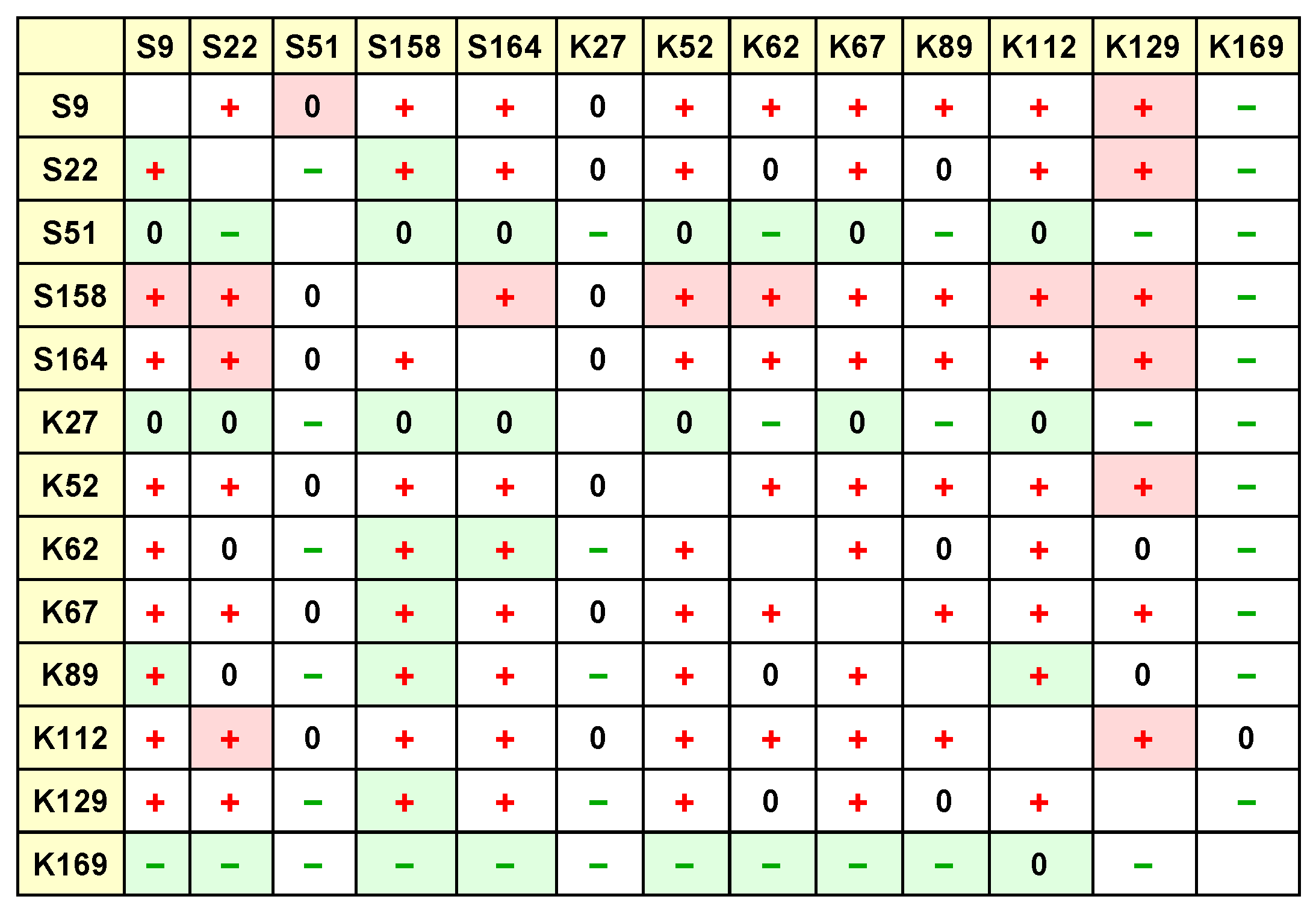
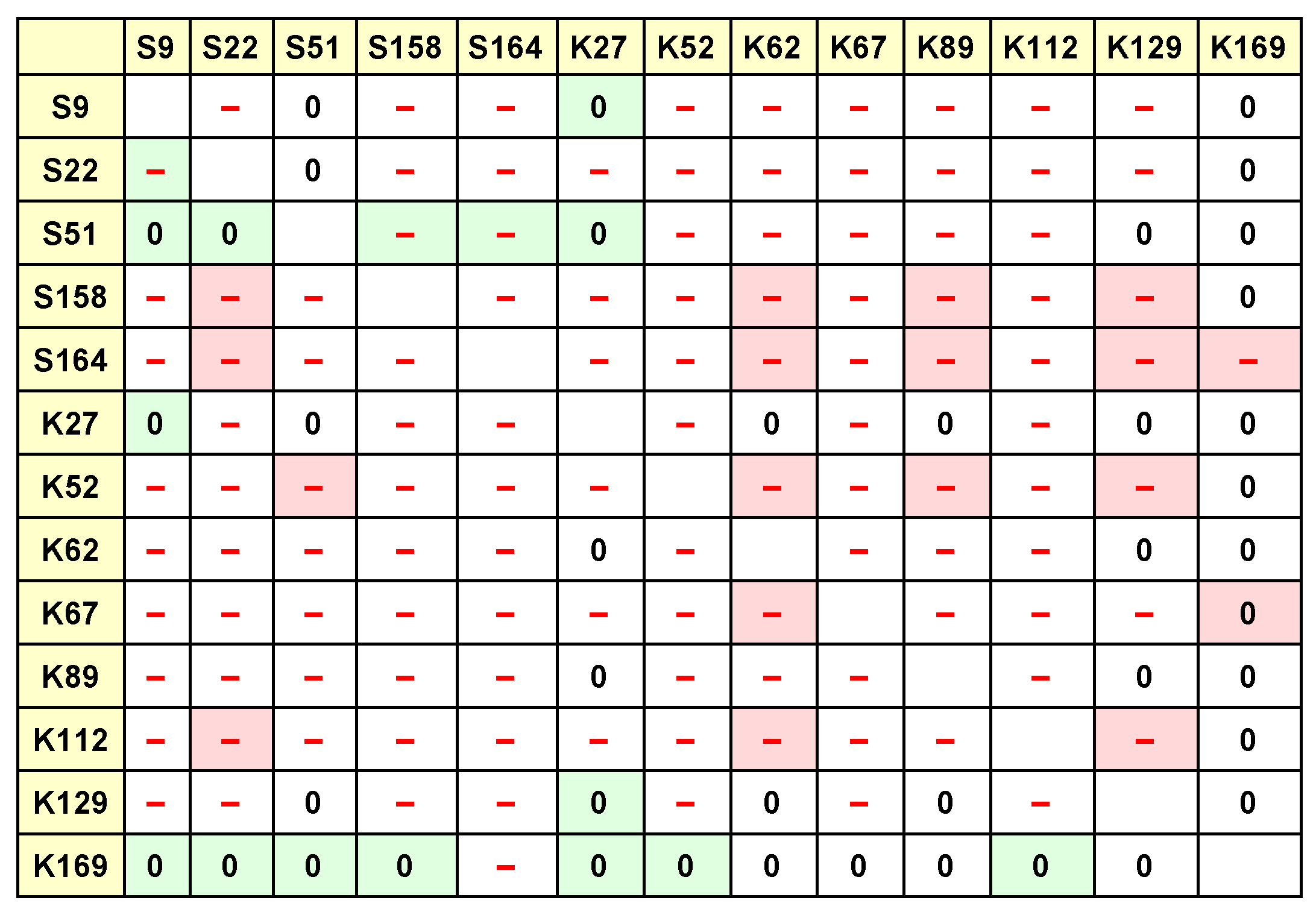
This test was done 13 times for each parameter, so that each of the strains was used once as the focal strain. The results of these tests are collected in the tables shown in Figure 1 and Figure 2. In these tables, each row collects the results of Tukey tests with a particular focal strain, e.g., the first row shows the results of tests where S9 was the focal strain, and the columns indicate the other strains being tested for interaction effects with S9.

3.1.2. Building the Competition Structures

Using the information gathered in Figure 1 and Figure 2, we represented the competition occurring between the SFIs using so-called tournament matrices. Such a matrix M for s species has dimensions s × s . If the species represented by row i outcompetes the species represented by column j, then M i j = 1 . On the other hand, if the species represented by row i is outcompeted by the species represented by column j, we have M i j = 1 . If i = j , then M i j = 0 . Using the information in Figure 1 and Figure 2, we can compile such a tournament or competition matrix. The question remains how precisely to do so.
We have two possibilities: to merge the information about the lag time λ and mineralization rate μ interaction effects, or to treat the parameters separately. The latter option is justified by considering that the parameters represent different biological attributes and different underlying processes [25]. This is most noticeable in their opposing effects on mineralization performance in particular; an increased parameter λ is considered a negative effect while an increased parameter μ is considered a positive effect.
This approach results in two competition matrices, the first based on lag time λ interaction effects, and the second based on mineralization rate μ interaction effects. We look in Figure 1 ( λ interaction effects) or Figure 2 ( μ interaction effects) for pairs of SFIs that appear to interact with each other, and check what kind of interaction appears to be taking place: is it positive or negative with respect to each of the SFIs?
This corresponds in Figure 1 and Figure 2 to both the cell entries and the cell background colours. The cell entries indicate which kind of difference (if any) exists between the control community and the R SFI = 2 community containing the particular species corresponding to the cell row and column. These relationships can be positive, negative, or not significant. The cell background colours indicate the difference (if any) between the R SFI = 1 community containing the species corresponding to the cell column, and the R SFI = 2 community containing the particular species corresponding to the cell row and column. These relationships can also be positive, negative, or not significant.
We then obtain the following matrices representing competition between the SFIs. When considering interactions based on lag time λ effects, the matrix reads:
M λ = 0 0 1 1 0 0 0 0 0 0 0 1 0 0 0 0 1 1 0 0 0 0 0 1 1 0 1 0 0 0 0 0 0 0 0 0 0 0 0 1 1 0 0 1 0 0 1 0 0 1 1 0 0 1 0 1 0 0 0 0 0 0 0 1 0 0 0 0 0 0 0 1 0 0 0 0 0 0 0 0 0 1 0 0 0 0 0 0 0 1 0 0 0 0 1 0 0 0 0 0 0 0 0 0 0 0 0 0 0 0 0 0 0 0 0 0 0 0 0 0 0 0 0 0 0 0 0 0 0 0 0 1 0 1 0 0 0 0 0 0 0 1 0 1 1 0 1 1 0 1 0 0 0 1 0 0 0 0 0 0 0 0 0 0 0 0 0 0 0
When considering interactions based on mineralization rate μ effects, the matrix has the form:
M μ = 0 0 0 0 0 0 0 0 0 0 0 0 0 0 0 0 1 1 0 0 0 0 0 1 0 0 0 0 0 0 0 0 1 0 0 0 0 0 0 0 1 0 0 0 0 0 1 0 1 0 1 0 0 1 0 0 0 0 0 1 0 1 0 1 1 0 0 0 0 0 0 0 0 0 0 0 0 0 0 0 1 0 0 0 0 1 0 1 0 1 0 0 0 0 1 1 0 1 0 1 0 1 0 0 0 0 0 0 0 0 0 1 0 0 0 0 1 0 0 0 1 1 0 1 0 0 0 0 0 0 0 1 0 0 0 0 0 1 0 0 0 1 0 0 0 0 1 1 0 1 0 0 0 1 0 0 0 0 0 0 1 0 0 0 1 0 0 0 0
An additional extension of our modelling approach that will bring it closer to reality is to also consider non-deterministic competition. Deterministic competition assumes that, if the competition structure specifies that A beats B, this will always occur: it will never be possible for B to beat A. This is reflected in the competition matrices M λ and M μ , which contain only 1’s (implying certain victory), −1’s (certain defeat) and 0’s (no competition). But this is not always realistic [30,31,32]. Variation between individuals can result in an individual of species A that is a particularly weak competitor, and an individual of species B that is a particularly strong competitor. If these two specific individuals meet, the outcome of the competition can be in doubt. It may be more realistic to specify a so-called winning probability [33,34]: the probability that A beats B. Including a winning probability allows for different competition outcomes to occur, and the value of the winning probability allows us to account for the relative strengths of the individuals.
Therefore we will also consider non-deterministic competition between the SFIs, not only in terms of its effects on the diversity and stability of the community (and possible subcommunity), but in comparison with the same effects due to deterministic competition. Our immediate question is then how to assign the winning probabilities to the different pairwise competitions.
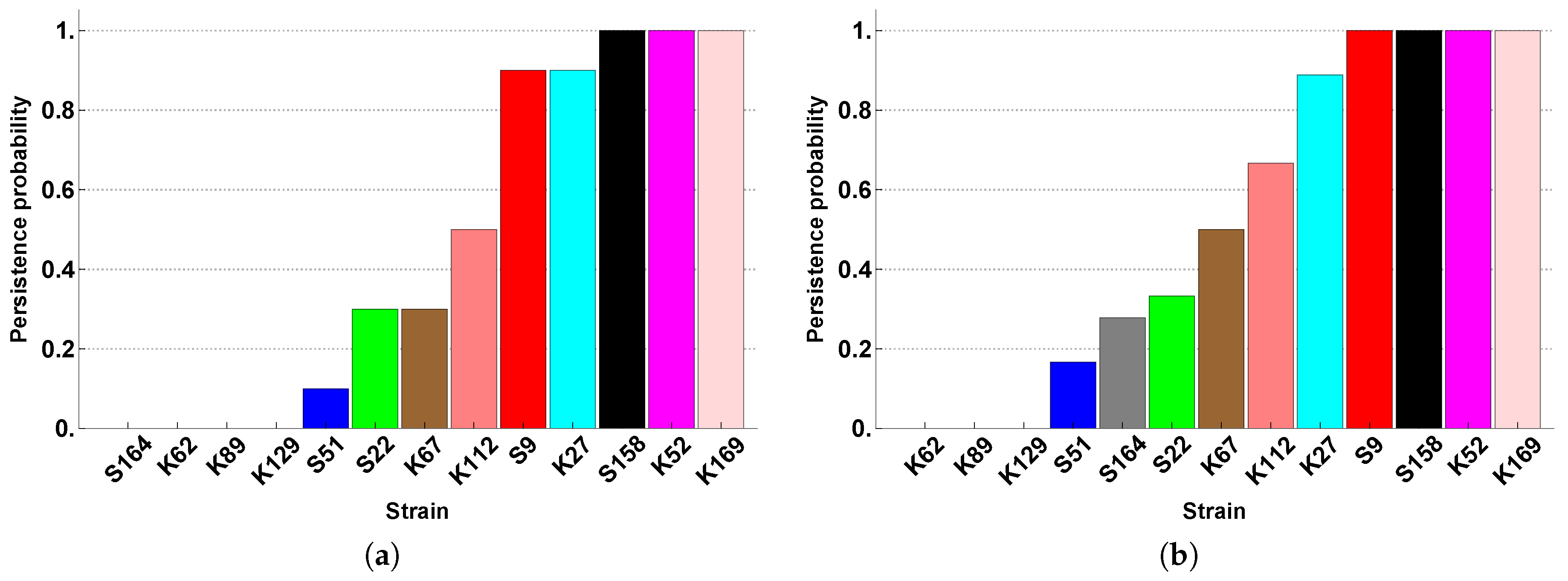
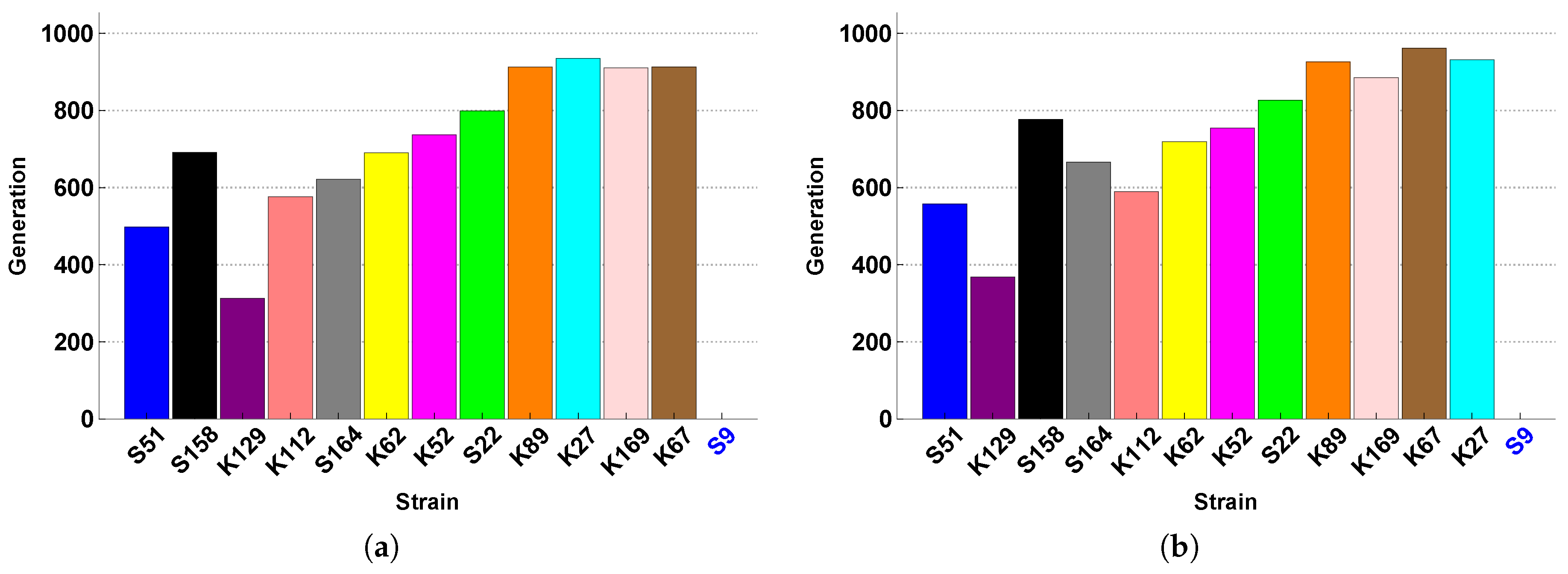
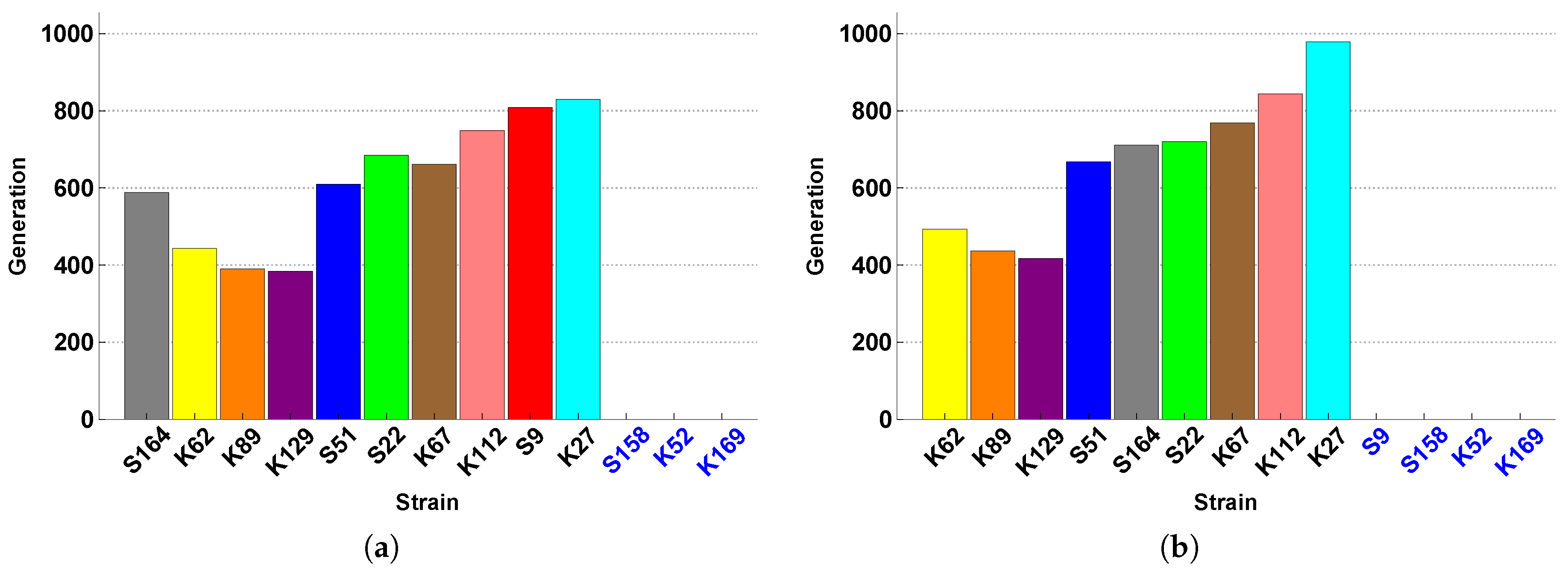
Using data related to the SFIs’ monoculture growth and survival curves, Vandermaesen et al. [11] classified the “intrinsic competitiveness” of the SFIs and on this basis grouped them into strong, intermediate and weak competitors. Using this information, we can assign winning probabilities to each pairwise competition based on the relative differences in intrinsic competitiveness between the two strains. For example, competition between a weak intrinsic competitor and a strong intrinsic competitor will most likely result in the success of the latter. It should also be clear that this winning probability should be higher than the winning probability assigned to an intermediate intrinsic competitor when faced with a weak intrinsic competitor. Using this approach, we replace the 1’s and −1’s populating our matrices M λ and M μ with rational numbers of absolute value less than 1, corresponding to the appropriate winning probability.
Using this approach, we obtain the following matrices representing non-deterministic competition. When considering interactions based on lag time λ effects, the matrix has the form:
M λ = 0 0 0.9 0.9 0 0 0 0 0 0 0 0.9 0 0 0 0 0.9 0.7 0 0 0 0 0 0.7 0.7 0 0.9 0 0 0 0 0 0 0 0 0 0 0 0 0.9 0.9 0 0 0.9 0 0 0.9 0 0 0.9 0.9 0 0 0.7 0 0.9 0 0 0 0 0 0 0 0.9 0 0 0 0 0 0 0 0 0 0 0 0 0 0 0 0 0 0.9 0 0 0 0 0 0 0 0.9 0 0 0 0 0.9 0 0 0 0 0 0 0 0 0 0 0 0 0 0 0 0 0 0 0 0 0 0 0 0 0 0 0 0 0 0 0 0 0 0 0 0 0.7 0 0.9 0 0 0 0 0 0 0 0.6 0 0.9 0.7 0 0.9 0.9 0 0.9 0 0 0 0.6 0 0 0 0 0 0 0 0 0 0 0 0 0 0 0
When considering interactions based on mineralization rate μ effects, the matrix has the form:
M μ = 0 0 0 0 0 0 0 0 0 0 0 0 0 0 0 0 0.9 0.7 0 0 0 0 0 0.7 0 0 0 0 0 0 0 0 0.9 0 0 0 0 0 0 0 0.9 0 0 0 0 0 0.9 0 0.9 0 0.9 0 0 0.7 0 0 0 0 0 0.7 0 0.6 0 0.9 0.7 0 0 0 0 0 0 0 0 0 0 0 0 0 0 0 0.9 0 0 0 0 0.9 0 0.9 0 0.9 0 0 0 0 0.9 0.7 0 0.9 0 0.7 0 0.7 0 0 0 0 0 0 0 0 0 0.7 0 0 0 0 0.7 0 0 0 0.9 0.6 0 0.9 0 0 0 0 0 0 0 0.7 0 0 0 0 0 0.7 0 0 0 0.6 0 0 0 0 0.9 0.9 0 0.9 0 0 0 0.6 0 0 0 0 0 0 0.7 0 0 0 0.7 0 0 0 0

3.2. Constructing the Individual-Based Model

To understand how the different competition structures affect the dynamics of the system, we consider the in silico counterpart of the synthetic community of 13 SFIs. We model this community using an individual-based approach, which we describe using an established standard protocol known as the ODD protocol [35].

3.2.1. Overview

Purpose

The aim of the model is to study how more realistic competition structures affect the in silico dynamics, particularly in terms of community diversity and stability, and investigate whether this approach can qualitatively reproduce the dynamics observed in similar in vitro studies, namely a stable and persisting subcommunity.

State Variables and Scales

The model is a two-dimensional representation of an experimental domain divided into a regular grid of size L × L = N , and populated by a community of 13 SFIs. We assign to each strain a numerical label between one and 13, in the order given in Section 3.1.1: S9, S22, S51, S158, S164, K27, K52, K62, K67, K89, K112, K129, K169. Each grid site is either occupied by a single individual, or is empty. Individuals are characterized by two state variables: grid position x , y and species identity s 1 , , 13 .

Process Overview

We consider an in silico microbial community that is initially placed on the grid with a random spatial distribution. The community’s initial species abundance distribution is completely even, to mimic the in vitro experimental set-up.
An individual can interact with its nearest neighbours, defined as those individuals in its von Neumann neighbourhood (the four grid cells with which it shares an edge). Three possible interactions can occur, representing the key demographic processes: reproduction, competition and mobility.
Reproduction can occur when an individual is located adjacent to an empty grid site, which is then filled with a new individual of the same species. In order to provide a form of mobility, all individuals can exchange their position with a nearest neighbour or move to a neighbouring empty site. Competition can occur between two neighbouring individuals that do not represent the same species. The outcome of the competition event is determined by the governing competition matrix; the defeated individual is removed from the grid and the grid site becomes empty.

Scheduling

The IBM proceeds using a modified version of the Gillespie algorithm [36], to determine which interaction occurs at each time step and calculate the interaction outcome. The algorithm iterates over the following steps:
(1)
Set time to t = 0 and set the event rate constants:
(a)
reproduction with rate constant μ
(b)
competition with rate constant σ
(c)
mobility with rate constant ϵ
(2)
Calculate the overall rate of events r = μ + σ + ϵ
(3)
Select an individual at random
(4)
Select one of the focal individual’s nearest neighbours at random
(5)
Select an interaction event with the following probabilities, by drawing a random number from the interval 0 , r :
(a)
reproduction with probability μ r
(b)
competition with probability σ r
(c)
mobility with probability ϵ r
(6)
Execute the selected interaction event on the selected individual (if permitted) and determine the outcome according to the governing rules:
(a)
reproduction occurs deterministically (it is always carried out if possible)
(b)
mobility occurs deterministically
(c)
competition can occur:
(i)
deterministically: the winner is determined by the appropriate entry (being 1 or 1 ) in the competition matrix M λ or M μ
(ii)
non-deterministically: a random number r c is drawn from the unit interval and compared to the appropriate winning probability M i j in the competition matrix M λ or M μ , where species i and species j are competing.
If M i j > 0 :
  • species i wins the competitive event if r c < M i j
  • species j wins the competitive event if r c > M i j
If M i j < 0 :
  • species i wins the competitive event if r c > | M i j |
  • species j wins the competitive event if r c < | M i j |
(7)
Update the grid according to the outcome of step 6
(8)
Update the time to t = t + 1
(9)
Return to step 3 and continue until t = t end
This procedure is repeated for a specified number of generations, where a generation is defined as the number of steps required for each cell to be the subject of on average one interaction.

3.2.2. Design Concepts

  • Emergence: the spatial patterns and population-level dynamics of the community emerge naturally from the interactions occurring between individuals.
  • Competition based on pairwise interaction effects: the competition scheme is constructed based on pairwise interaction effects, encoded in a competition matrix.
  • Non-deterministic competition: In addition to deterministic competition, we also investigate the effects of non-deterministic competition, where the victor of any competition event is not predetermined but is instead stochastic.
  • Interactions: individuals interact with each other and their environment by reproducing if located next to an empty site, exchanging sites with their neighbours, or competing with their neighbours.
  • Stochasticity: the stochasticity in the model arises from the initial spatial distribution of the grid; the interactions between individuals and the environment (reproduction); the interactions between individuals (mobility, competition); and from the non-deterministic competition.
  • Sensing: if selected for reproduction, individuals can sense whether their selected neighbouring site is empty; if so, they will reproduce. If the site is occupied by an individual, no reproduction will occur.
  • Observation: the data collected from the IBM includes the population count of each species, the community evenness and diversity, the spatial distribution of individuals, and their time to extinction. These are tracked for each time step.

3.2.3. Details

Initialization

The model is initialized with a random spatial distribution of individuals and empty sites. Initially, a certain proportion of grid sites is left empty; thus the system is initially below carrying capacity. The initial species abundance distribution is completely even, as is the typical approach in similar modelling studies [37,38,39]. Aside from the input variables, all other parameters used to initialize the model are fixed for all simulations, and are shown in Table 1. Note in particular that the mobility rate constant ϵ is set below the system’s critical mobility rate, above which extinctions are certain due to the interactions between individuals being insufficiently localized. It has been shown for models of this type that coexistence of all species is only possible when mobility remains low and therefore individuals can only interact over small spatial scales (in our case, with their nearest neighbours) [40].

3.2.4. Input

The model’s input is the competition matrix. There are four different matrices:
(i)
M λ : deterministic competition based on λ interaction effects (Matrix (2))
(ii)
M μ : deterministic competition based on μ interaction effects (Matrix (3))
(iii)
M λ : non-deterministic competition based on λ interaction effects (Matrix (4))
(iv)
M μ : non-deterministic competition based on μ interaction effects (Matrix (5))
For each of these initial settings, we run 200 replicate simulations.

3.3. In Silico Community Dynamics

3.3.1. Richness

To study the effects of the different types of competition on the diversity of the in silico synthetic community, we first examine the richness effects, by determining the number of surviving species after 1000 generations to see what levels of richness are maintained under the different competition structures.
In Figure 3, we show the probability of observing a certain species richness after 1000 generations. for deterministic and non-deterministic competition based on lag time λ interaction effects. With this competition structure, we observe monocultures very rarely in the deterministic case, and never in the non-deterministic case. We find final richness levels as high as eight (deterministic case) or nine species (non-deterministic case). In the deterministic case, approximately 70 % of simulations result in communities of five or six species, and the same for the non-deterministic case. The distribution of final richness is more skewed towards higher richness values for the non-deterministic case, indicating a stabilizing effect on the dynamics in terms of fewer extinctions and thus higher richness, an effect observed in other modelling studies comparing deterministic and non-deterministic effects [31]. This effect is not surprising, since non-deterministic competition results in fewer prey extinctions and more predator extinctions compared to deterministic competition, and thus decreasing extinction probabilities of the most vulnerable species.
The distribution of final richness for deterministic and non-deterministic competition based on mineralization rate μ interaction effects (Figure 4) is again more skewed towards higher richness values for the non-deterministic case, indicating a stabilizing effect on the dynamics in terms of fewer extinctions and thus higher richness. Additionally, higher richness levels are observed compared to the case of competition based on λ interaction effects. No monocultures are ever observed for competition based on μ interaction effects, and in fact community richness never drops below four (deterministic case) or five species (non-deterministic case). In the deterministic case, approximately 95 % of simulations result in communities of five or six species, in the non-deterministic case approximately 95 % of simulations result in communities of five, six or seven species.
Thus, in both cases ( λ and μ interaction effects), we find similar behaviour in terms of community richness as was observed for the in vitro synthetic community of Vandermaesen et al. [11], namely the establishment of a stable community of reduced richness compared to the initial inoculation of 13 SFIs.
The increased in silico community diversity in the case of competition based on mineralization rate μ interaction effects, compared to lag time λ effects, can be ascribed to a more balanced competition structure in the former case, and more specifically its relatively higher intransitivity. A competition structure is transitive if the constituent species can be ranked in a strict competitive hierarchy, and hence intransitivity refers to the lack of such a strict hierarchy [41]. This characteristic can be quantified for example using a measure of relative intransitivity proposed by Laird and Schamp [42], denoted by R I . This index takes values in the unit interval, with larger values corresponding to more intransitive competition structures. Using this index, we find that Matrix M μ is more intransitive than Matrix M λ , with a relative intransitivity of R I = 0 . 83 compared to R I = 0 . 80 , respectively.

3.3.2. Diversity

After observing the richness effects due to the different forms of competition, we now consider community diversity. We do so using the Leinster-Cobbold diversity index [43], an effective number index that also includes a sensitivity parameter q that determines how much weight is assigned to rare or common species. For q < 1 , more weight is given to rare species ( q = 0 corresponds to species richness), while for q > 1 more weight is given to common species. All species are weighed equally by their proportions for q = 1 [43].
For each of the four competition matrices, we calculate the Leinster-Cobbold diversity index over time, for different values of q, so that we may gather information about the composition and balance of the communities, as well as their changes in diversity as the different simulations evolve.
In Figure 5 we show the average Leinster-Cobbold diversity over time for deterministic and non-deterministic competition based on lag time λ interaction effects, for varying values of the sensitivity parameter q. With different values of q, we can infer changes in species richness (for low values of q), evenness (for high values of q) and diversity (for q = 1 ). Hence we calculate the diversity profiles for q 0 , 1 , 20 .
Initially, the community undergoes a sharp drop in evenness (seen in differences between the two curves for q > 0 relative to the q = 0 curve), while richness is maintained at its initial level. The time to the first species extinction is roughly similar for all replicates, namely around 250 generations. This period represents the time required for spiral spatial structures to begin to form (see Section 3.3.3), and the first species to be entirely surrounded by its predator(s) and killed off. Following the first extinction, others follow as they are enabled by the spatial structures as the species have aggregated sufficiently to begin to chase each other around the grid.
The q = 1 and q = 20 curves approach each other late in the simulation time, indicating that relatively high evenness is maintained for significant periods of time. However, the higher order diversities are significantly less than the zero order diversity (richness), indicating that in the later stages of the in silico experiments, multiple species continue to coexist but these communities are quite uneven, in agreement with the dynamics of the in vitro synthetic community [11]. Finally, we again observe a stabilizing effect when considering non-deterministic rather than deterministic in silico competition, in terms of time to first extinction and final community diversity.
In Figure 6, we compare the changes in diversity for communities subject to deterministic and non-deterministic competition based on mineralization rate μ interaction effects. Diversity is higher here than for the two previous competition matrices, for all values of q. Additionally, the communities are more even. Notably, in Figure 6 the q = 1 and q = 20 curves never overlap, indicating higher levels of evenness compared to the previous competition matrices which resulted in converging curves. This can also be inferred by the smaller distance between the q = 0 curve and the q > 0 curves in Figure 6, which indicates relatively more species coexisting in relatively more even communities. The minor stabilizing effect of non-deterministic competition compared to deterministic competition can also be observed in terms of diversity maintenance and time to first extinction.

3.3.3. Spatial Structures

These diversity effects, and the spatial dynamics underlying them, can also be observed in Figure 7, where we show two representative examples of the grid configuration at T = 1000 generations for non-deterministic competition based on lag time λ (Figure 7a) or mineralization rate μ (Figure 7b) interaction effects. As was observed in Figure 5 and Figure 6, competition based on the former results in more uneven communities than competition based on the latter. In the former case, sufficient species are present in sufficient numbers to form the spiral patterns characteristic of this type of individual-based models, which have been shown to help maintain coexistence [40]. These patterns also qualitatively resemble those observed in in vitro experiments where a similar synthetic community of SFIs was co-cultured with MSH1 in the presence of BAM [18]. The spiral formations also enable spatial refuges, which have been observed to support species coexistence by allowing vulnerable species to persist at low but still significant levels [44]. Such refuges can be observed for example in Figure 7b for multiple species.

3.3.4. Community Composition

Having studied community diversity effects, we can now turn our attention to the composition of these persisting subcommunities. In Figure 8, we show the persistence probability for each SFI for deterministic and non-deterministic competition based on lag time λ interaction effects. The results reflect the dynamics illustrated in Figure 7a: S9 is the dominant strain, but it is a member of a subgroup of SFIs that are present in the majority of the simulations. This is unsurprising, since S9 was the strongest competitor in the two competition structures based on λ interaction effects ( M λ and M λ ) and thus it is the dominant SFI in the persisting subcommunity, which we recall is quite uneven (see e.g., Figure 5 and Figure 7). In more than 80 % of the simulations, we observe the same SFIs persisting together: S9, K67, K169, K27 and K89. This is true for both the deterministic and non-deterministic competition cases.
Thus our model is able to qualitatively reproduce the in vitro dynamics of a persisting smaller subcommunity [11]. These dynamics have also been observed for communities of microbial species [18] as well as for communities of higher organisms [45,46].
Another subgroup of persisting SFIs is found for deterministic and non-deterministic competition based on mineralization rate μ interaction effects (Figure 9), once again matching qualitatively the dynamics observed in in vitro synthetic communities. The members of this subgroup are not entirely the same as for Figure 8. Instead we find K169, K52, S158, K27 and S9 coexisting in more than 80 % of the simulations. The strains in the persisting subcommunity are also more equal in terms of their persistence probabilities (and hence their extinction probabilities) than was the case for competition based on λ interaction effects (Figure 8). These SFIs are also more equally matched in terms of their competitive strengths (see M μ and M μ ). These factors result in these subcommunities being able to maintain significantly higher evenness levels than the other competition structures, as we noted when studying the diversity of these communities (Figure 6). The partial overlap in membership of the persisting subcommunities in the λ and μ cases may be ascribed to the fact that the dominance of a particularly adept competitor may be reflected in both the growth parameters under consideration.
Finally, we examine extinctions in our different communities. We have seen that extinctions are frequent, but generally limited to the same set of SFIs. In Figure 10, we show the average time to extinction for each SFI, for deterministic and non-deterministic competition based on lag time λ interaction effects. We note again that these are slightly longer for non-deterministic competition compared to deterministic competition, and always occur after an initial period of spiral formation (~300 generations). One strain, K129, collapses to extinction not long after spiral formation has commenced; this strain is the weakest in both competition structures. After it disappears, there is another lapse before extinctions recommence and thereafter proceed fairly regularly until the community is reduced to the persisting uneven subcommunity dominated by S9 (which never suffers any extinctions) and the other strains in small proportions.
For deterministic and non-deterministic competition based on mineralization rate μ interaction effects (Figure 11), we notice a reduction in extinction times compared to competition based on lag time λ interaction effects. This may seem counterintuitive given that we have already observed these communities to be more stable, however the key point is that fewer species go extinct. Those that do collapse to extinction do so more quickly, but this does not affect the stability of the persisting subcommunity. Now S9 is not the only SFI to never suffer extinctions, but it is joined by the other members of the persisting subcommunity (S158, K52 and K169), again indicating that this subcommunity is more even and thus more stable than in the cases of competition based on λ interaction effects.

4. Conclusions

We have studied the in silico counterpart of an in vitro synthetic community of 13 SFIs in co-cultures of varying richness with MSH1. These SFIs had been selected based on their potential for improving the BAM mineralization performance of MSH1 for bioaugmentation applications. We developed an IBM representing the in silico counterpart of this synthetic community, where competition structures were constructed based on pairwise competition outcomes, using data related to lag time λ and mineralization rate μ interaction effects in terms of mineralization performance.
Our model was able to recover the qualitative dynamics observed in in vitro experiments with similar synthetic sand filter communities: the majority of the community collapsing to extinction and a subcommunity persisting [11,18]. The memberships of these subcommunities were consistent, and their presence could be explained based on their attributes as represented in the competition matrices. The simulation outcomes were explained based on the underlying competition structures (notably by their intransitivity) and the resulting spatial dynamics. Our results highlight the importance of diversity and in particular evenness in stabilizing the community dynamics, in agreement with previous experimental results [47,48].
This work therefore serves as a proof-of-concept for using IBMs as in silico counterparts of in vitro synthetic communities, as we were able to find a qualitative agreement between the in silico and in vitro dynamics, despite the in vitro experiments not being expressly designed for modelling purposes. For example, it would also be informative for this purpose to examine in more detail the interactions between the SFIs, not just in terms of effects on BAM mineralization. This could be done, for example, by tracking the growth and survival of SFIs in pairwise co-cultures. Despite this, our model was able to retrieve the qualitative in vitro dynamics, allowing us to interrogate their development, and thereby illustrating the potential of this modelling approach for addressing ecological theories relating to synthetic communities.

Acknowledgments

The authors gratefully acknowledge the financial support of the Belgian Science Policy Office (IUAP contract P7/25) and the FP7 project BIOTREAT (EU grant 266039).

Author Contributions

A.J.D., J.M.B. and B.D.B. conceived and designed the in silico experiments; A.J.D. performed the experiments and analyzed the data; J.V., N.B. and D.S. contributed data and analysis tools; A.J.D. wrote the paper.

Conflicts of Interest

The authors declare no conflict of interest.

Appendix A

Figure A1. SFI monoculture growth curves on acetate [11].
Processes 06 00002 g0a1
Figure A2. SFI monoculture survival curves on acetate [11].
Processes 06 00002 g0a2

References

  1. Bairey, E.; Kelsic, E.; Kishony, R. High-order species interactions shape ecosystem diversity. Nat. Commun. 2016, 7. [Google Scholar] [CrossRef] [PubMed]
  2. Faust, K.; Raes, J. Microbial interactions: From networks to models. Nat. Rev. Microbiol. 2012, 10, 538–550. [Google Scholar] [CrossRef] [PubMed]
  3. Goers, L.; Freemont, P.; Polizzi, K. Co-culture systems and technologies: Taking synthetic biology to the next level. J. R. Soc. Interface 2014, 11. [Google Scholar] [CrossRef] [PubMed]
  4. De Roy, K.; Marzorati, M.; Van den Abbeele, P.; Van de Wiele, T.; Boon, N. Synthetic microbial ecosystems: An exciting tool to understand and apply microbial communities. Environ. Microbiol. 2014, 16, 1472–1481. [Google Scholar] [CrossRef] [PubMed] [Green Version]
  5. Verstraete, W.; Wittebolle, L.; Heylen, K.; Vanparys, B.; De Vos, P.; Van de Wiele, T.; Boon, N. Microbial resource management: The road to go for environmental biotechnology. Eng. Life Sci. 2007, 7, 117–126. [Google Scholar] [CrossRef]
  6. Hairston, D.; Huban, C.; Plowman, R.; Chemicals, S. Bioaugmentation: Put microbes to work. Chem. Eng. 1997, 104, 74–85. [Google Scholar]
  7. European Union. Directive 2006/118/EC of the European Parliament and of the council of 12 December on the protection of groundwater against pollution and deterioration. Off. J. Eur. Union 2006, 372, 19–31. [Google Scholar]
  8. Björklund, E.; Anskær, G.; Hansen, M.; Styrishave, B.; Halling-Sørensen, B. Analysis and environmental concentrations of the herbicide dichlobenil and its main metabolite 2, 6-dichlorobenzamide (BAM): A review. Sci. Total Environ. 2011, 409, 2343–2356. [Google Scholar] [CrossRef] [PubMed]
  9. Sørensen, S.; Holtze, M.; Simonsen, A.; Aamand, J. Degradation and mineralization of nanomolar concentrations of the herbicide dichlobenil and its persistent metabolite 2, 6-dichlorobenzamide by Aminobacter spp. isolated from dichlobenil-treated soils. Appl. Environ. Microbiol. 2007, 73, 399–406. [Google Scholar] [CrossRef] [PubMed]
  10. Thompson, I.; van der Gast, C.; Ciric, L.; Singer, A. Bioaugmentation for bioremediation: The challenge of strain selection. Environ. Microbiol. 2005, 7, 909–915. [Google Scholar] [CrossRef] [PubMed]
  11. Vandermaesen, J. Pesticide mineralization and effect of endogeneous community diversity on bioaugmentation in sand filters used in drinking water treatment. Ph.D. Thesis, KU Leuven, Leuven, Belgium, 2016. [Google Scholar]
  12. Esser, D.; Leveau, J.; Meyer, K. Modelling microbial growth and dynamics. Appl. Microbiol. Biotechnol. 2015, 99, 8831–8846. [Google Scholar] [CrossRef] [PubMed]
  13. Seshan, H.; Goyal, M.; Falk, M.; Wuertz, S. Support vector regression model of wastewater bioreactor performance using microbial community diversity indices: Effect of stress and bioaugmentation. Water Res. 2014, 53, 282–296. [Google Scholar] [CrossRef] [PubMed]
  14. Poschet, F.; Vereecken, K.; Geeraerd, A.; Nicolaï, B.; Van Impe, J. Analysis of a novel class of predictive microbial growth models and application to coculture growth. Int. J. Food Microbiol. 2005, 100, 107–124. [Google Scholar] [CrossRef] [PubMed]
  15. Widder, S.; Allen, R.; Pfeiffer, T.; Curtis, T.; Wiuf, C.; Sloan, W.; Cordero, O.; Brown, S.; Momeni, B.; Shou, W.; et al. Challenges in microbial ecology: Building predictive understanding of community function and dynamics. ISME J. 2016, 10, 1–12. [Google Scholar] [CrossRef] [PubMed]
  16. Nadell, C.; Foster, K.; Xavier, J. Emergence of spatial structure in cell groups and the evolution of cooperation. PLoS Comput. Biol. 2010, 6. [Google Scholar] [CrossRef] [PubMed]
  17. Momeni, B.; Waite, A.; Shou, W. Spatial self-organization favors heterotypic cooperation over cheating. eLIFE 2013, 2. [Google Scholar] [CrossRef] [PubMed]
  18. Horemans, B.; Vandermaesen, J.; Sekhar, A.; Springael, D. Aminobacter sp. MSH1 invades sand filter community biofilms while retaining 2,6-dichlorobenzamide degradation functionality under C and N limiting conditions. FEMS Microbiol. Ecol. 2017, 93. [Google Scholar] [CrossRef] [PubMed]
  19. Lehtola, M.; Miettinen, I.; Vartiainen, T.; Martikainen, P. Changes in content of microbially available phosphorus, assimilable organic carbon and microbial growth potential during drinking water treatment processes. Water Res. 2002, 36, 3681–3690. [Google Scholar] [CrossRef]
  20. Zwietering, M.; Jongenburger, I.; Rombouts, F.; Van’t Riet, K. Modelling of the bacterial growth curve. Appl. Environ. Microbiol. 1990, 56, 1875–1881. [Google Scholar] [PubMed]
  21. Buchanan, R.; Whiting, R.; Damert, W. When is simple good enough: A comparison of the Gompertz, Baranyi, and three-phase linear models for fitting bacterial growth curves. Food Microbiol. 1997, 14, 313–326. [Google Scholar] [CrossRef]
  22. Coleman, T.; Li, Y. On the convergence of interior-reflective Newton methods for nonlinear minimization subject to bounds. Math. Program. 1994, 67, 189–224. [Google Scholar] [CrossRef]
  23. Coleman, T.; Li, Y. An interior trust region approach for nonlinear minimization subject to bounds. SIAM J. Optim. 1996, 6, 418–445. [Google Scholar] [CrossRef]
  24. Vandermeeren, P.; Baken, S.; Vanderstukken, R.; Diels, J.; Springael, D. Impact of dry-wet and freeze-thaw events on pesticide mineralizing populations and their activity in wetland ecosystems: A microcosm study. Chemosphere 2016, 146, 85–93. [Google Scholar] [CrossRef] [PubMed]
  25. Ekelund, F.; Harder, C.; Knudsen, B.; Aamand, J. Aminobacter MSH1-mineralisation of BAM in sand-filters depends on biological diversity. PLoS ONE 2015, 10, e0128838. [Google Scholar] [CrossRef] [PubMed]
  26. Tonner, P.; Darnell, C.; Engelhardt, B.; Schmid, A. Detecting differential growth of microbial populations with Gaussian process regression. Genome Res. 2017, 27, 320–333. [Google Scholar] [CrossRef] [PubMed]
  27. Tukey, J. Comparing individual means in the analysis of variance. Biometrics 1949, 5, 99–114. [Google Scholar] [CrossRef] [PubMed]
  28. Haynes, W. Tukey’s Test. In Encyclopedia of Systems Biology; Dubitzky, W., Wolkenhauer, O., Cho, K.H., Yokota, H., Eds.; Springer: New York, NY, USA, 2013; pp. 2303–2304. [Google Scholar]
  29. Keuls, M. The use of the “studentized range” in connection with an analysis of variance. Euphytica 1952, 1, 112–122. [Google Scholar] [CrossRef]
  30. Mullon, C.; Fréon, P.; Cury, P.; Shannon, L.; Roy, C. A minimal model of the variability of marine ecosystems. Fish Fish. 2009, 10, 115–131. [Google Scholar] [CrossRef]
  31. Planque, B.; Lindstrom, U.; Subbey, S. Non-deterministic modelling of food-web dynamics. PLoS ONE 2014, 9, e108243. [Google Scholar] [CrossRef] [PubMed] [Green Version]
  32. Lindstrom, U.; Planque, B.; Subbey, S. Multiple Patterns of Food Web Dynamics Revealed by a Minimal Non-deterministic Model. Ecosystems 2017, 20, 163–182. [Google Scholar] [CrossRef]
  33. Ulrich, W.; Soliveres, S.; Kryszewski, W.; Maestre, F.; Gotelli, N. Matrix models for quantifying competitive intransitivity from species abundance data. Oikos 2014, 123, 1057–1070. [Google Scholar] [CrossRef] [PubMed]
  34. Moon, J. Topics on Tournaments in Graph Theory; Courier Dover Publications: Mineola, NY, USA, 2015. [Google Scholar]
  35. Grimm, V.; Berger, U.; Bastiansen, F.; Eliassen, S.; Ginot, V.; Giske, J.; Goss-Custard, J.; Grand, T.; Heinz, S.; Huse, G.; et al. A standard protocol for describing individual-based and agent-based models. Ecol. Model. 2006, 198, 115–126. [Google Scholar] [CrossRef]
  36. Gillespie, D. A general method for numerically simulating the stochastic time evolution of coupled chemical reactions. J. Comput. Phys. 1976, 22, 403–434. [Google Scholar] [CrossRef]
  37. Case, S.O.; Durney, C.H.; Pleimling, M.; Zia, R. Cyclic competition of four species: Mean-field theory and stochastic evolution. EPL Eur. Lett. 2010, 92. [Google Scholar] [CrossRef]
  38. Cheng, H.; Yao, N.; Huang, Z.G.; Park, J.; Do, Y.; Lai, Y.C. Mesoscopic interactions and species coexistence in evolutionary game dynamics of cyclic competitions. Sci. Rep. 2014, 4, 1–7. [Google Scholar] [CrossRef] [PubMed] [Green Version]
  39. Frachebourg, L.; Krapivsky, P.L.; Ben-Naim, E. Spatial organization in cyclic Lotka-Volterra systems. Phys. Rev. 1996, 54, 6186–6200. [Google Scholar] [CrossRef]
  40. Reichenbach, T.; Mobilia, M.; Frey, E. Mobility promotes and jeopardizes biodiversity in rock-paper-scissors games. Nature 2007, 448, 1046–1049. [Google Scholar] [CrossRef] [PubMed]
  41. Laird, R.; Schamp, B. Species coexistence, intransitivity, and topological variation in competitive tournaments. J. Theor. Biol. 2009, 256, 90–95. [Google Scholar] [CrossRef] [PubMed]
  42. Laird, R.; Schamp, B. Competitive intransitivity, population interaction structure, and strategy coexistence. J. Theor. Biol. 2015, 365, 149–158. [Google Scholar] [CrossRef] [PubMed]
  43. Leinster, T.; Cobbold, C. Measuring diversity: The importance of species similarity. Ecology 2012, 93, 477–489. [Google Scholar] [CrossRef] [PubMed] [Green Version]
  44. Daly, A.; Baetens, J.; De Baets, B. The impact of resource dependence of the mechanisms of life on the spatial population dynamics of an in silico microbial community. Chaos 2016, 26, 123121. [Google Scholar] [CrossRef] [PubMed]
  45. Dunne, J.; Williams, R. Cascading extinctions and community collapse in model food webs. Philos. Trans. R. Soc. Lon. B Biol. Sci. 2009, 364, 1711–1723. [Google Scholar] [CrossRef] [PubMed]
  46. Ebenman, B.; Jonsson, T. Using community viability analysis to identify fragile systems and keystone species. Trends Ecol. Evol. 2005, 20, 568–575. [Google Scholar] [CrossRef] [PubMed]
  47. De Roy, K.; Marzorati, M.; Negroni, A.; Thas, O.; Balloi, A.; Fava, F.; Verstraete, W.; Daffonchio, D.; Boon, N. Environmental conditions and community evenness determine the outcome of biological invasion. Nat. Commun. 2013, 4. [Google Scholar] [CrossRef] [PubMed]
  48. Daly, A.J.; Baetens, J.M.; De Baets, B. The impact of initial evenness on biodiversity maintenance for a four-species in silico bacterial community. J. Theor. Biol. 2015, 387, 189–205. [Google Scholar] [CrossRef] [PubMed]
Figure 1. Tukey test results for the lag time λ . Each row collects the results of Tukey tests with a particular focal strain, the columns then indicate the strains that were tested for interaction effects with it. The entry in cell i , j indicates the difference (if any) between the R SFI = 2 community containing species i and species j, and the control R SFI = 0 community: “+” indicates the R SFI = 2 parameter values were significantly larger than the R SFI = 0 values, “–” indicates they were significantly smaller, and “0” indicates no significant difference. The background colour of cell i , j indicates the difference (if any) between the R SFI = 2 community containing species i and species j, and the R SFI = 1 community containing species j: green indicates the R SFI = 2 parameter values were significantly smaller than the R SFI = 1 values, red indicates they were significantly larger, and no colour indicates no significant difference.
Processes 06 00002 g001
Figure 2. Tukey test results for the mineralization rate μ . Each row collects the results of Tukey tests with a particular focal strain, the columns then indicate the strains that were tested for interaction effects with it. The entry in cell i , j indicates the difference (if any) between the R SFI = 2 community containing species i and species j, and the control R SFI = 0 community: “+” indicates the R SFI = 2 parameter values were significantly larger than the R SFI = 0 values, “–” indicates they were significantly smaller, and “0” indicates no significant difference. The background colour of cell i , j indicates the difference (if any) between the R SFI = 2 community containing species i and species j, and the R SFI = 1 community containing species j: green indicates the R SFI = 2 parameter values were significantly larger than the R SFI = 1 values, red indicates they were significantly smaller, and no colour indicates no significant difference.
Processes 06 00002 g002
Figure 3. Probability of observing a particular species richness after 1000 generations for (a) deterministic and (b) non-deterministic competition based on λ effects. Probabilities calculated from 200 replicates.
Processes 06 00002 g003

(a)(b)
Figure 4. Probability of observing a particular species richness after 1000 generations for (a) deterministic and (b) non-deterministic competition based on μ effects. Probabilities calculated from 200 replicates.
Processes 06 00002 g004

(a)(b)
Figure 5. Mean diversity profiles (Leinster-Cobbold index) for q { 0 , 1 , 20 } , for (a) deterministic and (b) non-deterministic emergent competition based on λ effects. Mean and standard deviation calculated from 200 replicates.
Processes 06 00002 g005

(a)(b)
Figure 6. Mean diversity profiles (Leinster-Cobbold index) for q { 0 , 1 , 20 } , for (a) deterministic and (b) non-deterministic emergent competition based on μ effects. Mean and standard deviation calculated from 200 replicates.
Processes 06 00002 g006

(a)(b)
Figure 7. Examples of in silico communities at T = 1000 generations with emergent non-deterministic competition based on (a) λ effects, and (b) μ effects.
Processes 06 00002 g007

(a)(b)
Figure 8. Probability of finding each strain in the community after 1000 generations) for (a) deterministic and (b) non-deterministic emergent competition based on λ effects.
Processes 06 00002 g008

(a)(b)
Figure 9. Probability of finding each strain in the community after 1000 generations) for (a) deterministic and (b) non-deterministic emergent competition based on μ effects.
Processes 06 00002 g009

(a)(b)
Figure 10. Mean time to extinction per strain for (a) deterministic and (b) non-deterministic emergent competition based on λ effects. Blue labels indicate strains for which no extinctions occurred. Means calculated from 200 replicates.
Processes 06 00002 g010

(a)(b)
Figure 11. Mean time to extinction per strain for (a) deterministic and (b) non-deterministic emergent competition based on μ effects. Blue labels indicate strains for which no extinctions occurred. Means calculated from 200 replicates.
Processes 06 00002 g011

(a)(b)
Table 1. Parameters of the individual-based model of 13 SFIs.
ParameterDescriptionValue
LGrid side length200
øInitial proportion of empty sites0.1
μ Reproduction rate constant1
σ Competition rate constant1
ϵ Mobility rate constant4.25
TNumber of generations evolved1000

