Article

Species Coexistence in Nitrifying Chemostats: A Model of Microbial Interactions

INRA, UR50, Laboratoire de Biotechnologie de l’Environnement, Narbonne F-11100, France
*
Author to whom correspondence should be addressed.
Processes 2016, 4(4), 51; https://doi.org/10.3390/pr4040051
Submission received: 26 September 2016 / Revised: 5 December 2016 / Accepted: 7 December 2016 / Published: 14 December 2016

Abstract

:
In a previous study, the two nitrifying functions (ammonia oxidizing bacteria (AOB) or nitrite-oxidizing bacteria (NOB)) of a nitrification reactor—operated continuously over 525 days with varying inputs—were assigned using a mathematical modeling approach together with the monitoring of bacterial phylotypes. Based on these theoretical identifications, we develop here a chemostat model that does not explicitly include only the resources’ dynamics (different forms of soluble nitrogen) but also explicitly takes into account microbial inter- and intra-species interactions for the four dominant phylotypes detected in the chemostat. A comparison of the models obtained with and without interactions has shown that such interactions permit the coexistence of two competing ammonium-oxidizing bacteria and two competing nitrite-oxidizing bacteria in competition for ammonium and nitrite, respectively. These interactions are analyzed and discussed.

1. Introduction

The well-known “competitive exclusion” principle states that, at equilibrium, the number of coexisting competing species cannot exceed the number of growth-limiting resources available to them [1,2]. However, in natural systems, the number of coexisting species often exceeds the number of limiting resources [3]. This phenomenon is often referred to as the “paradox of the plankton” [4]. Theoretical and experimental studies of a chemostat with time-invariant operating conditions have shown that two microbial populations in competition for a single substrate cannot coexist: the slower-growing species in the given operating conditions will be washed out [5]. In such a case, coexistence is predicted theoretically for discrete values of the chemostat dilution rate only when the curves of the specific growth rate, as a function of limiting nutrient concentration, cross. The dilution rate must have exactly the value at which the specific growth rates of the two populations in the chemostat are equal. However, this type of coexistence is structurally unstable and cannot be realized in practice because of random fluctuations in the chemostat dilution rate and in the physico-chemical parameters. To bridge the gap between mathematical theory and real life, a variety of mathematical models have been developed over recent decades. In all such models, assumptions about the idealized chemostat have been modified (cf. for instance [6,7,8,9,10]). Some studies have relied on non-equilibrium conditions to promote species diversity by preventing competitive equilibrium. One such example is the variability in resource supply ratios: when nutrients were supplied to the chemostat in pulses, oscillations in the abundance of species prevented the establishment of competitive equilibrium and permitted the coexistence of a greater number of species than the number of growth-limiting resources [11,12]. In the same way, some studies have explained coexistence in chemostats by the heterogeneity of the medium or by variations in solid retention times [8] while others have considered that more than one single resource is available [13]. However, only very few studies related to the chemostat have pointed out that microbial interactions other than competition can also lead to steady-state coexistence. When such a situation was considered, only direct interactions based on the approach called Generalized Lotka–Volterra equations were used and no consideration was given to resources (cf., for instance [14] for a recent study). In particular, for Lotka–Volterra models, it has been established that coexistence is possible when intra-specific competition is greater than inter-specific competition. The ecological mechanism behind this result is that the self-limiting growth of the most competitive species leaves some resource available for other less competitive species. While some progress has been made towards integrating positive interactions into contemporary theory [15,16,17], competition and predation still dominate ecological thinking about interspecific interaction [18,19,20]. The fact is that, to allow coexistence in mass-balance models, it is either necessary (i) to consider identical kinetics parameters for all species (which is actually what we could call a “singular case” and which would have, as a consequence, the observation of exactly the same dynamic behavior for all species) or (ii) to add direct interaction terms between species concentrations as in the Lotka–Volterra model, in addition to the dependence with respect to resource concentrations.
Recently, interest in the study of species interactions has been renewed regarding the modern high-throughput molecular techniques available: together with modeling, they appear as a very promising way of investigating how ecosystems function. Available models are based on network theory and statistical data analysis [21]. However, these proposed models usually do not consider resources and only describe, statically, species interactions within the ecosystem of interest.
Roughly speaking, all the available models could be classified as either Biodiversity-Equivalent or Functionally-Equivalent. Biodiversity-Equivalent Models (BEM) aim to provide models able to explain/predict/simulate biodiversity, typically as species interacting together within a microbial ecosystem; while Functionally-Equivalent Models (FEM) are designed to predict function performances of an ecosystem. The classic chemostat model is typically a FEM while the neutral model could be classified as a BEM. Very few microbial-ecosystem models available in the literature have been designed to integrate both diversity and functional considerations. In [22,23,24], such models were proposed for anaerobic digestion. However, both hypothesize that the different biomasses are only in competition for the substrate and do not include terms involving direct interactions: thus, unless the growth functions are identical, the competitive exclusion principle applies and only one species will survive if the system is simulated for a long enough period of time [25]. In addition, like other studies published in the fields of ecology or mathematics, these studies remain essentially theoretical and were not confronted to data (cf., for instance [26,27]).
The aim of the model proposed in the present paper is to include both diversity and functional considerations and to validate such a model on data obtained within real experiments. More specifically, we present here a modification of the classic model of a chemostat. It is based on Lotka–Voltera equations and takes into account biotic interactions which can occur between species in a microbial community (i.e., which represent inter- and intra-species interactions). Not only does this model integrate states of more than one species per function (number of biological reactions) but it also integrates the dynamics of available resources. This model was confronted to data obtained from a nitrifying chemostat operated for two years under time-varying inputs. Notice, however, that for technical reasons related to the parameter identification step, only the signs and the order of magnitude of interaction terms between species could be obtained and not their precise values (we will come back in detail on this important point in Section 2.5).
Nitrification is an aerobic two-step microbial process (thus involving only two “functions”) in which ammonium is oxidized to nitrate by two distinct groups of chemolithoautotrophic bacteria. Aerobic ammonium-oxidizing bacteria (AOB) first oxidize ammonium to nitrite and then aerobic nitrite-oxidizing bacteria (NOB) oxidize the nitrite to nitrate [28,29]. During the two year experiments used in the present study, both functional measurements (i.e., concentrations in ammonium, nitrite and nitrate concentrations) and population measurements (i.e., total biomass concentration and relative abundances) of the bacteria present in the chemostat were made by Single Strand Conformation Polymorphism. In a previous work, using an original mathematical approach, a functional community assignation (i.e., in AOB or NOB community) was performed for each phylotype detected in the chemostat [30,31]. In the present work, a microbial interaction model is optimized on the kinetics of the two most abundant phylotypes of each functional community. In this way, we obtain a virtual web of interactions linking four different species present in the nitrifying community. The results obtained in this way show that the web of interactions can prevent competitive exclusion and can explain the coexistence of the phylotypes as observed through the available measurements realized on the nitrifying chemostat as predicted in [26,27].

2. Materials and Methods

2.1. Nitrifying Chemostat Conditions

The experimental set-up operated over two years consisted of two continuously-mixed 6.5 L (working volume) all-glass chemostats inoculated beforehand with activated sludge from the municipal sewage treatment plant of Coursan (Aude, France). The air flow-rate was maximum in order to ensure good fluidization and provide enough oxygen which was never limiting for the nitrification process; the pH was measured and maintained at around 7 by the automatic addition of an alkaline solution. Both chemostats were fed with a synthetic mineral medium composed of ammonium sulfate (its concentration varying from 0.5 to 2 g·L−1) as the nitrogen source, complemented with a mineral solution.

2.2. Microbial Community Measurements

During the experiments which lasted 525 days, two kinds of population measurements were made: the first was the determination of the total biomass present in the chemostats; the second consisted of the determination by Single Strand Conformation Polymorphism (SSCP) of the abundances of the different species contained in the total biomass. Except for some well-identified periods, the experiment was run in duplicate and both chemostats behaved similarly. For this reason, in the present study we concentrate on the results obtained from only one device (the chemostat denoted as “chemostat B” in [31]). The main results of this monitoring—on average over the 525 days of experiments—were (i) 40% of the total biomass was represented by the most abundant AOB; (ii) the most abundant NOB represented less than 10% of the total biomass; (iii) the two most abundant AOB and the two most abundant NOB represented more than 55% of the total biomass.

2.3. Model Development

The model developed in this study is based on mass balance equations for a conventional, completely-mixed chemostat initiated from the pioneering work of Monod and of Novick and Szilard (cf. [32,33]). It is described by the following set of differential equations:
{ X ˙ = ( μ ( S ( t ) ) D ( t ) ) X ( t ) S ˙ = ( S i n ( t ) S ( t ) ) D ( t ) 1 Y μ ( S ( t ) ) X ( t )
where the dot above a letter stands for the time-derivative, S and X represent the concentrations of nutrient (or substrate) and biomass, respectively. Sin denotes the concentration of the nutrient in the input flow, with dilution rate D. The function µ(S(t)) is the growth rate of the population and the yield factor is Y. Thereafter, to simplify the notations, the time-dependence of variables is often omitted.
This standard dynamic model of a chemostat can be extended easily to a 2-step nitrifying bioprocess as follows:
{ X ˙ A = ( μ A ( S 1 ) D ) X A X ˙ B = ( μ B ( S 2 ) D ) X B S ˙ 1 = ( S i n S 1 ) D 1 Y A μ A ( S 1 ) X A S ˙ 2 = S 2 D + 1 Y A μ A ( S 1 ) X A 1 Y B μ B ( S 2 ) X B S ˙ 3 = S 3 D + 1 Y B μ B ( S 2 ) X B ,
where XA and XB represent the concentrations of AOB and NOB respectively, while μ A ( S 1 ) and μ B ( S 2 ) are the growth rates of XA and XB, respectively. As suggested in [31], they are supposed to be Monod functions and are thus written as μ A ( S 1 ) = μ m a x 1 S 1 S 1 + K s 1 and μ B ( S 2 ) = μ m a x 2 S 2 S 2 + K s 2 .
From this point onwards, this model will be referred to as “model #1”. This nitrifying chemostat model can then be modified as follows to take into account microbial interactions:
{ X ˙ i | i = 1 .. n A + n B = [ μ i ( . ) ( 1 + j = 1 j = n A + n B a i j X j ) D ] X i S ˙ 1 = ( S i n S 1 ) D 1 Y A i = 1 i = n A [ μ i ( S 1 ) ( 1 + j = 1 j = n A + n B a i j X j ) X i ] S ˙ 2 = S 2 D + 1 Y A i = 1 i = n A [ μ i ( S 1 ) ( 1 + j = 1 j = n A + n B a i j X j ) X i ] 1 Y B i = n A + 1 i = n A + n B [ μ i ( S 2 ) ( 1 + j = 1 j = n A + n B a i j X j ) X i ] S ˙ 3 = S 3 D + 1 Y B i = n A + 1 i = n A + n B [ μ i ( S 2 ) ( 1 + j = 1 j = n A + n B a i j X j ) X i ] ,
where aij represents the influence of the species j on the growth rate of species i. This influence can be positive, negative or nil according to the sign and the value of aij.
From this point onwards, this last model, including intra- and interspecific interaction terms, will be referred to as “model #2”. This interaction coefficient structure (aij) corresponds to that of the well-known Lotka–Volterra model which is a widely used model in general ecology. Our model differs from the classic Lotka–Volterra model in that it is coupled to a mass-balance model (the classic chemostat model) which includes resource dynamics. Because linear systems are easier to identify, using a linear “species by species” relationship allows a simpler way of predicting species interactions. However, in doing so, the influence of resource density is neglected. An example of the use of such an interaction coefficient structure to describe microbial interactions within a cheese microbial community is given in [34]. It should also be noted that, for a given species j, the interaction terms are assumed to be constant. We are aware that this assumption may be questionable from a purely biological point of view. However, as explained in the next section, only the sign of interactions will finally be characterized. Said differently, we rather characterize the distributions in which these parameters live, instead of their precise values.

2.4. Identification of the Parameters of Microbial Interaction

The parameters of model #1, optimized to match experimental data in [31] are recalled in Table 1.
The identification of microbial interactions was done with the help of the model #2 described by Equation (3). To do so, we have kept only the two major species of each group: recall the four most abundant phylotypes (two AOBs and two NOBs) represented about 55% of total biomass. In order to ensure a viable compromise between the complexity of the model (notably the number of parameters to be identified) and the capability of optimization algorithms to converge within a reasonable computing time, only two phylotypes in competition for one of the two substrates S1 or S2, were studied for each of the two nitrifying functions, thus considering only four species in total.
Considering the model described by Equation (3) with nA = nB = 2, there still remains a large number of parameters to be identified (interaction parameters between the four considered species, that is to say 16 parameters, plus the degrees of freedom of the kinetics, representing eight additional parameters, thus a total of 24 parameters). To minimize this number, we adopt, in the present study, a kind of “neutral” hypothesis in considering that within a function, all the species exhibit identical kinetics and that the only difference in growth was due to their interaction. This assumption can be justified taking into account the following arguments. Without interactions, considering the same growth rates for either AOBs or NOBs, all species would exhibit exactly the same dynamics: their coexistence would be “guaranteed” (of course assuming that initial biomass concentrations are nonzero). However, it is not what is observed in practice (cf. the data we use from [31]: we will come back on these data later on but it will be clearly shown that the dynamics of AOB1 and AOB2, and of NOB1 and NOB2, are significantly different). Now, with different growth rates and again no interactions, the competitive exclusion principle applies and coexistence is simply not possible. Again, it is actually not what is observed in practice. In other terms, the kinetics associated with each species—the rate at which species i consumes its main limiting resource— should be considered to be modulated by interactions.
Referring to model #2 and assuming we assign i = 1 and 2 for AOB1 and AOB2, respectively, and i = 3 and 4 for NOB1 and NOB2, respectively, we have:
μ 1 ( S 1 ) = μ 2 ( S 1 ) and μ 3 ( S 2 ) = μ 4 ( S 2 )
Thus, instead of 24, we are now left with 20 parameters needing identification. Using model #1 as a “provider” of data (by simulation) for model #2, the identification of the interaction parameters of model #2 can now be framed in terms of an optimization problem, as follows: find the parameters of μ i | i = 1 .. 4 under the constraints (4) and the interaction parameters aij such that the outputs of model #2 match the simulated outputs of model #1 (S1, S2, S3 and XT = XA + XB = AOB1 + AOB2 + NOB1 + NOB2). This optimization problem can be reformulated as follows: find the parameters of μ i | i = 1 .. 4 under the constraints (4) and the interaction parameters aij in the model #2 such that:
( μ A ( S 1 ( t ) ) D ( t ) ) X A ( t ) | m o d e l # 1         = i = 1 i = n A [ μ i ( S 1 ( t ) ) ( 1 + j = 1 j = n A + n B a i j X j ( t ) ) X i ( t ) ]         D ( t ) ( X 1 ( t ) + X 2 ( t ) ) | m o d e l # 2
and
( μ B ( S 2 ( t ) ) D ( t ) ) X B ( t ) | m o d e l # 1         = i = n A + 1 i = n A + n B [ μ i ( S 2 ( t ) ) ( 1 + j = 1 j = n A + n B a i j X j ( t ) ) X i ( t ) ]         D ( t ) ( X 3 ( t ) + X 4 ( t ) ) | m o d e l # 2
To insist on the fact that these constraints must hold for all t, we included the time-dependance of variables. For this problem, we used the Sum of Square Residuals (SSR) criterion consisting of the sum of the squared difference of the terms on the left and the terms on the right in the previous expressions—(5) and (6)—over the considered 525 days of experiments.
To solve this problem, we adopted a Monte-Carlo-like approach (cf. Appendix A):
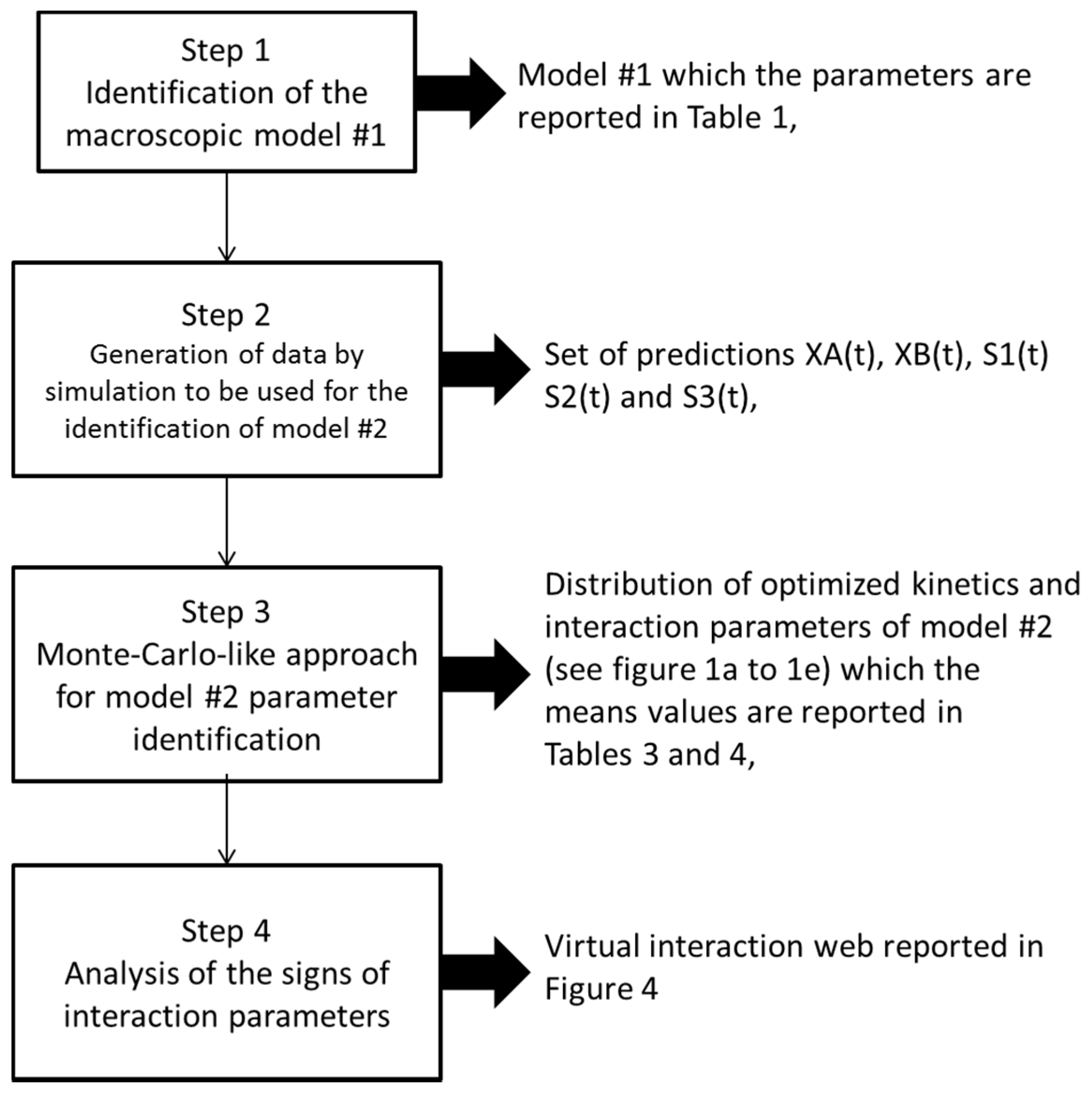
  • First, we randomly ran 2000 optimizations (using more did not improve the results (i.e., did not enable us to further decrease the final confidence intervals computed for each identified parameter) with different initial conditions for the parameters to be estimated (all unknown parameters in the right-hand terms of the above equations). In other terms, we identified all the parameters with different initial conditions 2000 times;
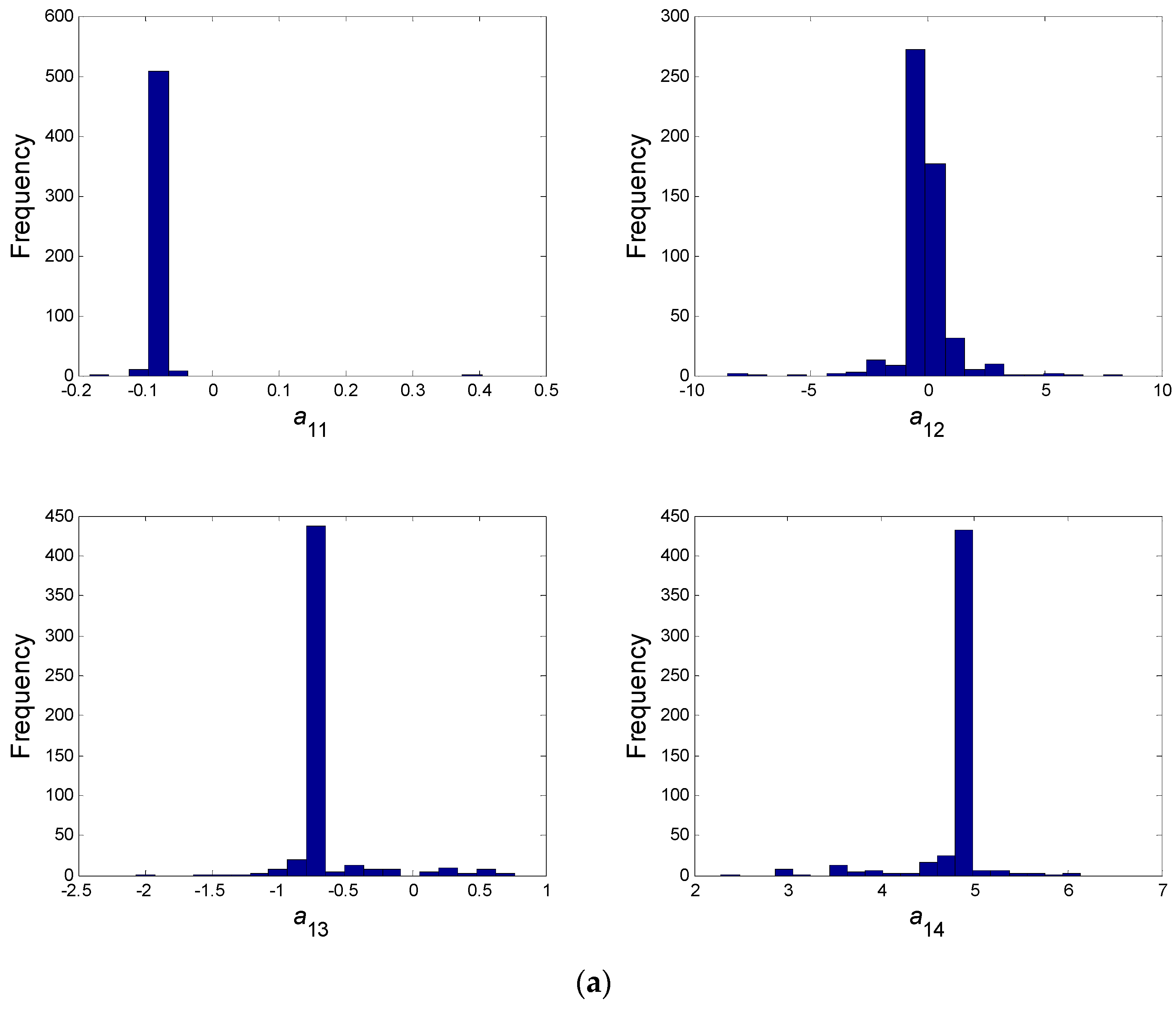
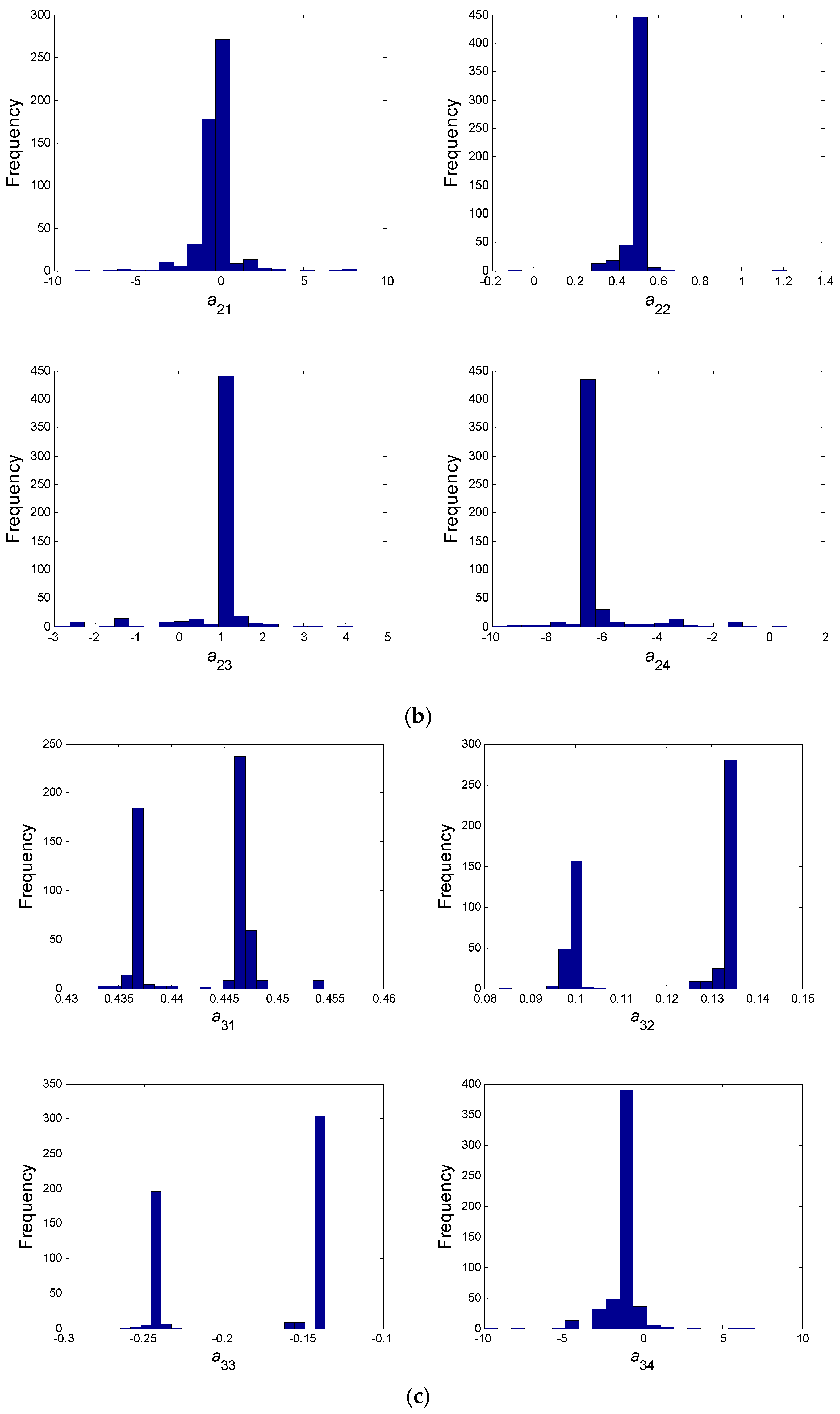
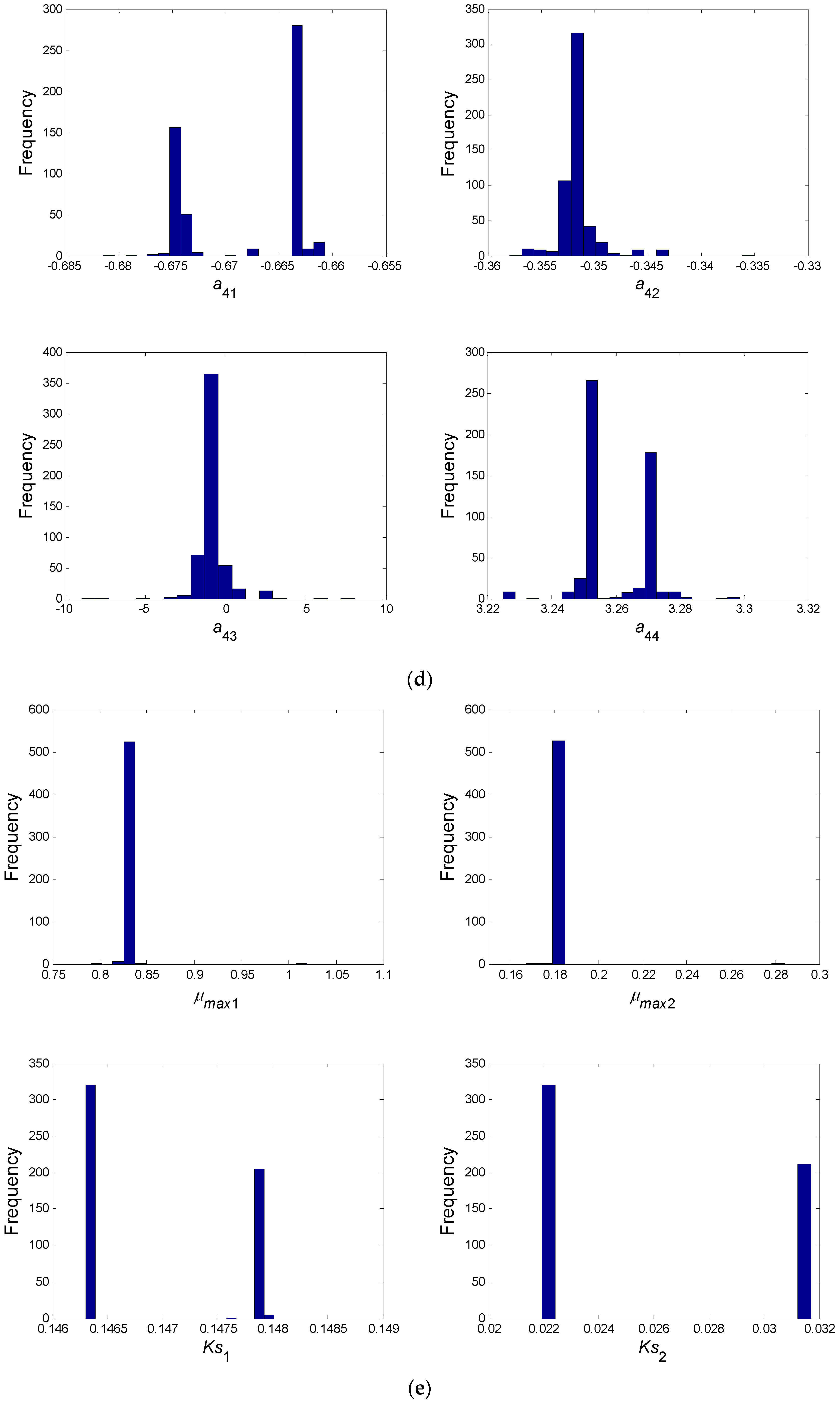
  • In a second step, we have proceeded to a statistical analysis of the results, keeping only the best sets of optimized parameters that are the sets for which the SSR was, at most, 5% greater than the best solution over the 2000 optimizations. Instead of keeping only the best one, we proceeded in this way for two reasons: (i) The problem to be solved is complex, notably because the model is nonlinear and the number of unknowns is high. Thus, we did not necessarily obtain the same parameter values for each of the 2000 optimizations. In other words, the problem we consider here is said to be “non-identifiable”. It means that, given the structure of the model considered, a unique set of parameters cannot be found from the available data. In other words, there exist “hidden relationships” between parameters—possibly nonlinear—which prevent the optimization algorithm from converging towards a unique global minimum and, consequently, from delivering a unique set of optimized parameters (cf. for instance [35] or [36] for more information about this concept); (ii) in the results, either the parameters are centered around 0 with a large standard deviation (indicating either no interaction between the corresponding species or an undetermined interaction) or the signs of the identified interactions are always the same whatever the sets of optimized parameters considered and, thus, the proposed statistical analysis of the results to obtain qualitative insights about microbial interactions in the ecosystem is considered without considering precise parameter values. In the sequel, this procedure will be referred to as a “Monte-Carlo-like” approach;
  • Finally, following the procedure described above, 520 sets of optimized parameters over the 2000 runs were kept and analyzed. The results are presented and discussed in the following sections.

2.5. Remarks

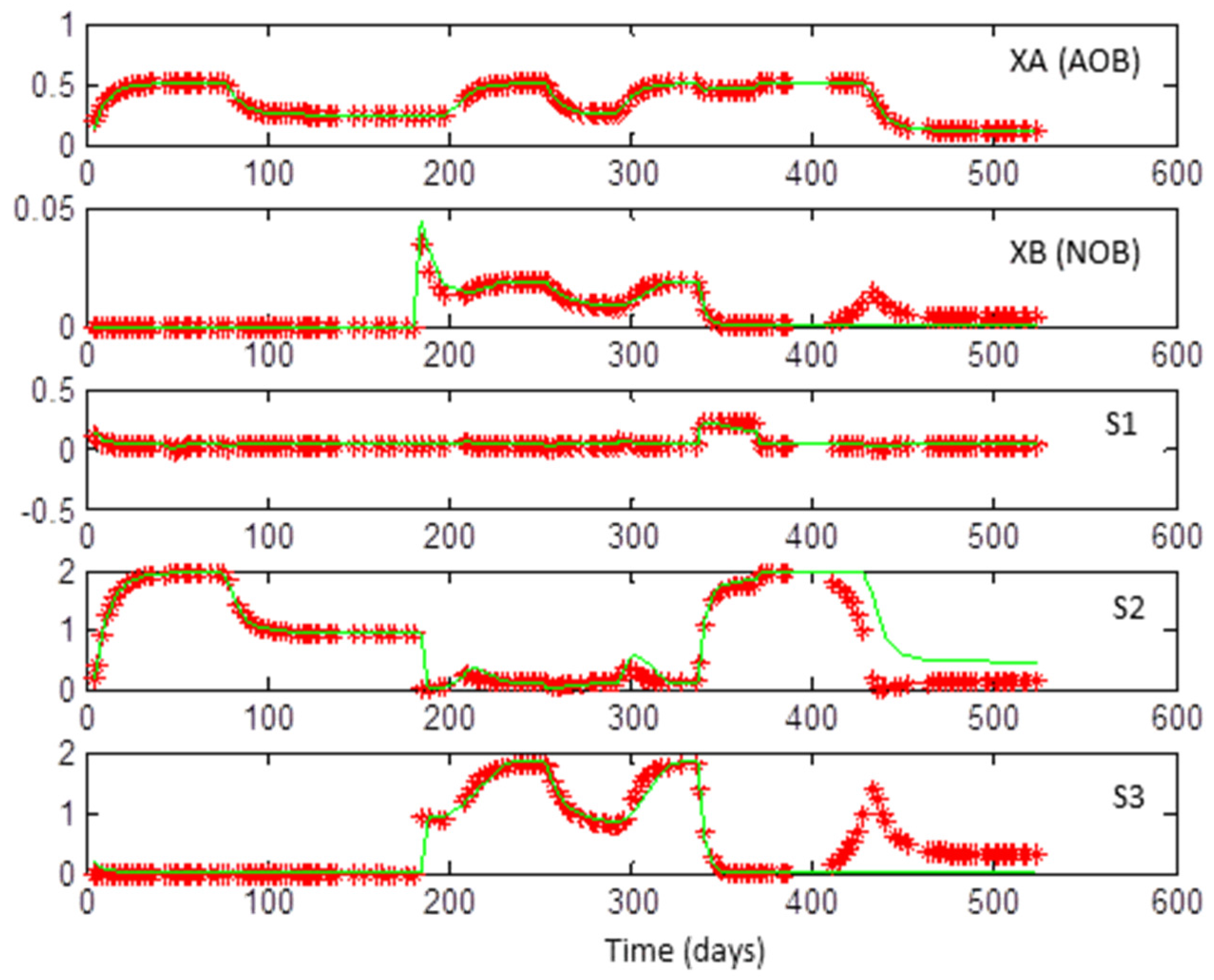
  • An important question that may arise is the following: Why are outputs of the model #1 used in the optimization problem (in the evaluation of the left-hand terms of (5) and (6)) rather than experimental data available in [31]? The essential reason is that experimental data are corrupted by noise. It is well known in system identification that, by definition, noise is not informative. Since the problem posed here is very sensitive to data (recall, in particular, that the problem is non-identifiable), it is better to use noise-free data [35,36]. Here, completely noise-free data generated with the simulation of model #1 (itself optimized with respect to real data in Dumont’s work, cf. [31]) were used instead of using real data.
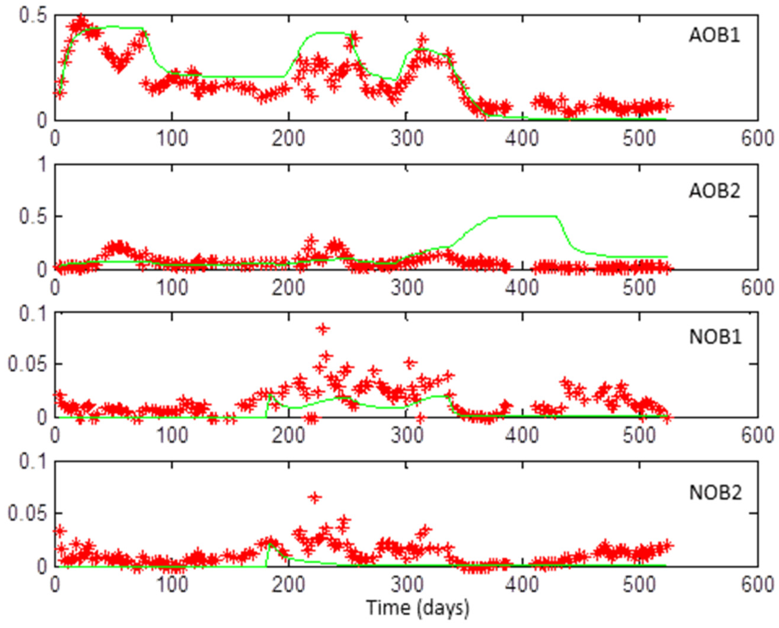
  • As noted before, the sum of the four species considered within model #2 represented on average about 55% of the total biomass in the experiments published in [31]. For practical purposes, before proceeding to parameter identification, the relative abundances of these four species were re-normalized in such a way that their sum equaled the total biomass as measured in the experiments. In other words, considering that model #2 (which describes the dynamics of four species) is equivalent to saying that the two biological reactions involved are now only attributable to these four species and that the remaining detected species (41 − 4 = 37 in the data considered over the 525 days of experiments) are simply ignored.
  • Finally, another question that may be posed is related to the parameter identification results. One may ask whether a solution to the optimization problem should be to fix all interaction parameters to zero or not. In fact, this solution cannot give a better fit than any other because there is no reason to have XA = X1 + X2 and XB = X3 + X4. In other terms, individual concentrations of the four AOBs and NOB species are taken explicitly into account in the criterion used to fit model #2 parameters while only the total biomass concentration was considered in the optimization criterion to optimize model #1 parameters. Since the criterions are different, model parameters (i.e., interaction terms) are tuned so that the differences between the two sides of Equations (5) and (6) are minimized.
A schematic representation of the procedure followed in this study is presented in the appendix.

3. Results

3.1. Coexistence of 2 + 2 Species on 1 + 1 Growth-Limiting Resources by Microbial Interaction

The distribution of the parameter values (interactions and kinetics parameters) over the 520 optimized parameter sets are plotted in Figure 1a–e. As shown in these figures, most parameters are randomly distributed around mean values following Gaussian-like distributions while others present bimodal distributions. In addition, even if their precise values are not informative (for the identifiability reasons we mentioned above), it should be noted that the intervals in which the mean values of the kinetics parameters (cf. distributions in Figure 1e and mean values reported in Table 2) live appear to be in accordance with those reported in the literature (cf. [37]).
Table 2 and Table 3 present the mean values for the microbial interaction parameters together with the kinetics parameters identified.
Concerning its main outputs, the interaction model presents a very good fit with the simulated data obtained from model #1 (cf. Figure 2).
As explained in the Materials and Methods section, we can compare the experimental data and the predictions for the dynamics of AOB1, AOB2, NOB1 and NOB2 that can be simulated using model #2. However, notice that the behavior over time of these species, e.g., the concentrations of these species, may vary depending on the sets of interaction and kinetics parameters identified. Indeed, recall that the best 520 parameter sets have been kept for the statistical analysis of results. All permit a good fit with the outputs of both models #1 and #2 (otherwise, they would not have been kept after the parameter identification process) while predicting different individual behavior for the two AOB and the two NOB species. In other words, the set of optimized parameters is not unique and one may only compare simulations of model#2 using a particular set of parameters among the 520 sets that have been kept for the statistical analysis. Such a specific set is given in Table 4.
The predictions of model #2 using this specific set of parameters together with the experimental data presented in [31], are plotted in Figure 3. Because of the uncertainty of measurements, it is clear that only the qualitative behavior of these simulation results should be considered within the context of the actual work.
Whatever the species considered, it should be noted that the models with interactions always better fitted data than the predictions of the same models in which interactions were fixed at 0. This result can easily be understood given that a model with more tuning parameters than another should be able to deliver better predictions. In addition, from an ecological point of view, when microbial interactions are not considered (fixed to 0), the model does not allow the coexistence of 2 + 2 species on 1 + 1 growth-limiting resources as predicted by the theory of the chemostat. Yet this coexistence was observed in practice (cf. the measurements of species abundances reported in [31] or in Figure 3 here above). The divergence between experimental data and estimates of the models between t = 375 days and t = 430 days for the AOB2 can be explained by a washout of the chemostat in reaction to the increase in the flow rate made on t = 337 days which was already mentioned in [31].

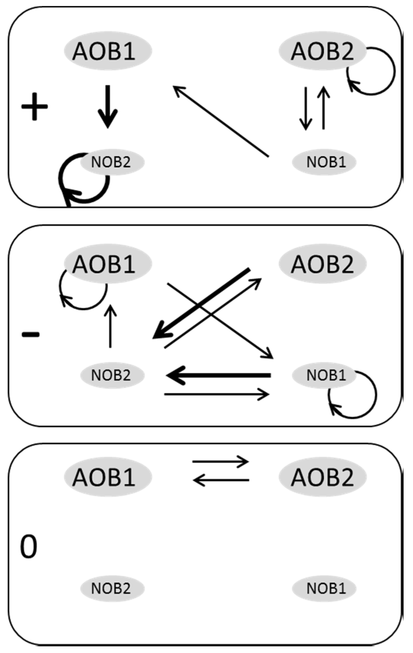
3.2. Web of Microbial Interactions

On the basis of the identified microbial interactions model, we can build a web of microbial interactions linking the different phylotypes with their mean values as reported in Table 3.
Over the network of 16 interactions contained in the model #2, six are positive and eight are negative (cf. Figure 4). Only two almost-null interactions emerge. Concerning interactions between both AOB, neither competition nor facilitation was highlighted. However, strong intra-specific facilitation appears for the second AOB with a22 = +0.47. These two ammonium-oxidizing phylotypes exercise interactions of both facilitation and competition with both of the nitrite-oxidizing phylotypes. However, a stronger, mostly negative interaction (a24 = −6.36, a34 = −1.23 and a14 = +4.81) of all bacteria with NOB2 is to be noted which seems to be compensated for by a strong intra-specific relationship of NOB2 with itself (a44 = +3.26/Bimodal distribution). Concerning interactions between the two nitrite-oxidizing phylotypes, NOB1 imposes a high negative interaction on NOB2 (a34 = −1.23) while NOB2 forces a moderately negative relationship on NOB1 (a43 = −0.84). A moderate intra-specific competition appears for NOB1 (a33 = −0.18/Bimodal distribution) whereas a high intra-specific facilitation appears for NOB2 (a44 = +3.26). Concerning the type of interactions which maintain NOB in relation to AOB, a supplementary “balanced structure” appears. Indeed, if we take into account only the signs of interaction, there are as many positive as negative interactions. Whereas NOB1 presents fairly positive interactions with AOBs (a31 = +0.44 and a32 = +0.11/Bimodal distributions), NOB2 seems to interact rather negatively with AOBs (a41 = −0.67/Bimodal distribution and a42 = −0.35).
The actual results underline positive interactions only from AOB1 to NOB2 and AOB2 to NOB1 (cf. Figure 4). However, in the same time, negative interactions were observed between AOB1/NOB1 and AOB2/NOB2. In addition, competition was not observed between AOBs, whereas there was strong competition between NOBs.

4. Discussion

Monitoring over two years the population and functioning of a nitrifying chemostat under time-varying environmental conditions highlighted the coexistence of numerous species in a culture fed with ammonium as the nitrogen source. The data acquired indicate that, throughout the period of the study, there occurred rapid, significant shifts in the structure of bacterial population. A comparison with the experimental data of the two proposed models—with and without microbial interactions—has shown that microbial interactions lead to the coexistence of a greater number of species than predicted by the classical chemostat model in which the competitive exclusion principle applies. In macrosystem ecology, several models have been presented that represent intra- and inter-species interactions in food webs (cf. [15]). The most frequently-used model is the multispecies Lotka–Volterra. For a given species, it is based on a linear relationship between its growth rate parameters and the population of each member of the community. For instance, with respect to real data, this model has been used to describe microbial interactions within a cheese microbial community [34]. In the present study, we combined this interaction coefficient structure (aij) with a classic model of a nitrifying chemostat. To the best of our knowledge, it is one of the first models of microbial ecosystems which tries (i) to integrate the dynamics of several interacting bacterial in the chemostat and (ii) tunes its parameters to match data together with the modeling of functions (here, nitritation and nitratation). To date, the prime focus of predator–prey models has been applied to models describing food webs in which non-trophic interactions, such as competition, facilitation and biotic disturbance, have been largely ignored [15]. Because food web models focus—by their very nature—exclusively on trophic interactions, they assume implicitly that predation is the most important process regulating community structure and dynamics. Moreover, while models of complex food webs incorporate only competition among species, they generally ignore any form of resource competition among the species (cf. [38,39]). This can be explained by the fact that, in food webs, nutrients flow via trophic links and, for this reason, trophic interactions have a fundamental character due to the principle of mass conservation.
Concerning the “competitive exclusion principle” (i.e., the “paradox of the plankton”), a variety of mathematical models have been proposed over recent decades, as underlined in the introduction. However, once again, intra- as well as inter-specific interactions have not been taken into consideration and in all such models, the assumptions about an idealized chemostat have been modified to permit coexistence [10]. Some studies have relied on non-equilibrium conditions to promote species diversity by preventing competitive exclusion. Examples include variability in resource supply ratios. When nutrients were supplied to the chemostat in pulses, oscillations in the abundance of species prevented competitive equilibrium from occurring and led to the coexistence of a greater number of species than the number of growth-limiting resources (cf. [11,12]). The only recent theoretical study that does not contradict the competitive exclusion principle and, at the same time, permits what has been called “practical coexistence” with neither variations in the environment nor any interaction through species or foodweb is [25]. In this study, it is the diversity itself—which is considered to be high, as observed in most microbial natural ecosystems—which creates the conditions under which the system can allow species coexistence over an arbitrarily long period of time as long as growth rate functions for each species are close enough. Their conclusions were that possibly we observe ecosystems that are never close to an equilibrium. Some other studies explain coexistence in a chemostat by variation in solid retention times [8]. Only a very small number of studies have taken an interest in microbial interactions. In [10], Hebeler et al. explained coexistence in the chemostat as a result of metabolic by-products. In their study, they found experimental evidence for a specific metabolic property of Staphylococcus aureus which produced acetate (a by-product). In a mixed culture, this can have an activating effect (as a secondary substrate) as well as an inhibiting effect (by reducing pH) on the other species. In [12], it is shown, using a modeling study, that the number of coexisting species may exceed the number of limiting resources when internal system feedbacks induce oscillations and chaos. This occurs if the species displace each other in a cyclic fashion. However, this can be considered as a very rare phenomenon—for not saying singular—since it requires a very precise parameterization of the parameters of community members [7]. Nevertheless, few authors have considered interactions empirically and directly in microbial ecology, even though a long history of experimental and theoretical ecology has elucidated how predation interacts with other non-trophic processes—including interference competition, facilitation, disturbance, environmental stress, productivity and recruitment—to regulate species distribution and abundance (cf. [40,41]). Finally, the microbial interaction model proposed here makes it possible to obtain a virtual web of interactions linking the main species present in the ecosystem of interest. It appears that we have underlined a “balanced interacting-structure model” in the sense that there are as many positive as negative interactions in the virtual web.
The experiments reported in [31] in the chemostat clearly show the coexistence of bacteria performing the same function (41 phylotypes observed) for a long period (525 days). These results can be compared to those presented in [42]. These authors considered a two-competitor/one prey model and explained the coexistence of the two competitors by density-dependent mortality for one of the two species. The interaction web also shows preferential “couples” or “pairs” of micro-organisms (AOB1/NOB2 and AOB2/NOB1) that are not “interchangeable” (AOB1/NOB1 and AOB2/NOB2) and which exhibit negative interactions. With a model built at a population level, it is obviously very difficult to interpret biologically direct interaction terms aij. However, an example of a configuration in which such interactions could develop is as follows. Consider—for some unknown reason—that AOB1 and NOB1, on the one hand, and AO2 and NOB2, on the other hand, develop specific interactions (for instance in forming ”bi- specific” flocs). Because of their proximity, AOB1 and NOB1 (resp. AOB2 and NOB2) could develop specific biotic interactions while each pair would now be in competition with the other. If such an explanation remains highly speculative, it is not inconceivable that such interactions are developing in a complex natural ecosystem.
There is no competition for NH4+ between AOBs. Unfortunately, some interactions, such as NOB2/NOB2, as well as the low abundance of NOBs compared to AOBs, often underlined in the literature, cannot be explained.
In conclusion, we developed a new model of nitrifying chemostat to study the interactions within two functional groups of four species: two AOBs and two NOBs. The network of virtual interactions obtained can explain the coexistence of these 2 + 2 species on 1 + 1 growth-limiting resources. Of the perspectives deriving from this work, one could design other more complete models including multiple functional groups of organisms, such as nitrifying and denitrifying heterotrophs, phosphorus-accumulating organisms, etc. In addition, this study focused on the effects of interactions within a single trophic level (bacteria). Effects of the presence of higher trophic levels, for instance predation by virus or protozoa, could also be considered. However, in all these cases, a number of issues, including the identification of a large number of model parameters, need to be dealt with from a theoretical viewpoint before such more complicated models can be developed.

Acknowledgments

All experiments and Maxime Dumont’s PhD grant were financed by INRA.

Author Contributions

All authors conceived and designed the experiments; Maxime Dumont performed the experiments; all authors analyzed the data; Jérôme Harmand and Maxime Dumont designed models. Jérôme Harmand wrote the paper.

Conflicts of Interest

The authors declare no conflict of interest.

Appendix A

Procedure followed for the identification of the virtual interaction web.
Figure A1. Identification procedure.
Processes 04 00051 g005

References

  1. Gause, G.F. Vérifications Expérimentales de la Théorie Mathématique de la Lutte pour la vie; Hermann et Cie: Paris, France, 1935. [Google Scholar]
  2. Hardin, G. The competitive exclusion principle. Science 1960, 131, 1292–1297. [Google Scholar] [CrossRef] [PubMed]
  3. Chesson, P. Mechanisms of maintenance of species diversity. Ann. Rev. Ecol. Syst. 2000, 31, 343–366. [Google Scholar] [CrossRef]
  4. Hutchinson, G.E. The paradox of the plankton. Am. Nat. 1961, 95, 137–145. [Google Scholar] [CrossRef]
  5. Hansen, S.R.; Hubbell, S.P. Single-nutrient microbial competition: qualitative agreement between experimental and theoretically forecast outcomes. Science 1980, 207, 1491–1493. [Google Scholar] [CrossRef] [PubMed]
  6. Aarssen, L.W. High productivity in grassland ecosystems: effected by species diversity or productive species? OIKOS 1997, 80, 183–184. [Google Scholar] [CrossRef]
  7. Schippers, P.; Verschoor, A.M.; Vos, M.; Mooij, W.M. Does “supersaturated coexistence” resolve the “paradox of the plankton”? Ecol. Lett. 2001, 4, 404–407. [Google Scholar] [CrossRef]
  8. Saikaly, P.E.; Oerther, D.B. Bacterial competition in activated sludge: Theoretical analysis of varying solids retention times on diversity. Microb. Ecol. 2003, 48, 274–284. [Google Scholar] [CrossRef] [PubMed]
  9. Sree Hari Rao, V.; Raja Sekhara Rao, P. Mathematical models of the microbial populations and issues concerning stability. Chaos Solitons Fractals 2005, 23, 657–670. [Google Scholar] [CrossRef]
  10. Hebeler, J.; Schmidt, J.K.; Reichl, U.; Flockerzi, D. Coexistence in the chemostat as a result of metabolic by-products. J. Math. Biol. 2006, 53, 556–584. [Google Scholar]
  11. Sommer, U. Comparison between steady state and non-steady state competition: experiments with natural phytoplankton. Limnol. Oceanogr. 1985, 30, 335–346. [Google Scholar] [CrossRef]
  12. Huisman, J.; Weissing, F.J. Coexistence and resource competition. Nature 2000, 4, 407–432. [Google Scholar]
  13. Schmidt, J.K.; Riedele, C.; Regestein, L.; Rausenberger, J.; Reichl, U. A novel concept combining experimental and mathematical analysis for the identification of unknown interspecies effects in a mixed culture. Biotechnol. Bioeng. 2011, 108, 1900–1911. [Google Scholar] [CrossRef] [PubMed]
  14. Marino, S.; Baxter, N.T.; Huffnagle, G.B.; Petrosino, J.F.; Schloss, P.D. Mathematical modeling of primary succession of murine intestinal microbiota. PNAS 2014, 111, 439–444. [Google Scholar] [CrossRef] [PubMed]
  15. Berlow, E.L.; Neutel, A.M.; Cohen, J.E.; De Ruiter, P.C.; Enbenman, B.O.; Emmerson, M.; Fox, J.W.; Jansen, V.A.A.; Jones, J.I.; Kokkoris, G.D.; et al. Interaction strengths in food webs: Issues and opportunities. J. Anim. Ecol. 2004, 73, 585–598. [Google Scholar] [CrossRef]
  16. Bascompte, J.; Jordano, P.; Olesen, J.M. Asymmetric coevolutionary networks facilitate biodiversity maintenance. Science 2006, 312, 431–433. [Google Scholar] [CrossRef] [PubMed] [Green Version]
  17. Michalet, R.; Brooker, R.W.; Cavieres, L.A.; Kikvidze, Z.; Lortie, C.J.; Pugnaire, F.I.; Valiente-Banuet, A.; Callaway, R.M. Do biotic interactions shape both sides of the humped-back model of species richness in plant communities? Ecol. Lett. 2006, 9, 767–773. [Google Scholar] [CrossRef] [PubMed]
  18. Brooker, R.W.; Maestre, F.T.; Callaway, R.M.; Lortie, C.L.; Cavieres, L.A.; Kunstler, G.; Liancourt, P.; Tielborger, K.; Travis, J.M.J.; Anthelme, F.; et al. Facilitation in plant communities: The past, the present, and the future. J. Ecol. 2008, 96, 18–34. [Google Scholar] [CrossRef]
  19. Gross, K. Positive interactions among competitors can produce species-rich communities. Ecol. Lett. 2008, 11, 929–936. [Google Scholar] [CrossRef] [PubMed]
  20. Haruta, S.; Kato, S.; Yamamoto, K.; Igarashi, Y. Intertwined interspecies relationships: Approaches to untangle the microbial network. Environ. Microbiol. 2009, 11, 2963–2969. [Google Scholar] [CrossRef] [PubMed]
  21. Faust, K.; Raes, J. Microbial interactions: From networks to models. Nat. Rev. 2012, 10, 538–550. [Google Scholar] [CrossRef] [PubMed]
  22. Ramirez, I.; Volcke, E.; Rajinikantha, R.; Steyer, J.P. Modeling microbial diversity in anaerobic digestion through an extended ADM1 model. Water Res. 2009, 43, 2787–2800. [Google Scholar] [CrossRef] [PubMed]
  23. Tapia, E.; Donoso, A.; Cabrol, L.; Alves, M.; Pereira, A.; Rapaport, A.; Ruiz, G. A methodology for coupling DGGE and mathematical modelling: Application in bio-hydrogen production. In Proceedings of the 13th IWA World Congress on Anaerobic Digestion, Santiago de Compostela, Spain, 25–28 June 2013.
  24. Sbarciog, M.; Vande Wouwer, A. Start-up of multispecies anaerobic digestion systems: Extrapolation of the single species approach. Math. Comput. Model. Dyn. Syst. 2014, 20, 87–104. [Google Scholar] [CrossRef]
  25. Rapaport, A.; Dochain, D.; Harmand, J. Long run coexistence in the chemostat with multiple species. J. Theor. Biol. 2009, 257, 252–259. [Google Scholar] [CrossRef] [PubMed]
  26. Lobry, C.; Harmand, J. A new hypothesis to explain the coexistence of n species in the presence of a single resource. C. R. Biol. 2006, 329, 40–46. [Google Scholar] [CrossRef] [PubMed]
  27. Saito, Y.; Miki, T. Species coexistence under resource competition with intraspecific and interspecific direct competition in a chemostat. Theor. Popul. Biol. 2010, 78, 173–182. [Google Scholar] [CrossRef] [PubMed]
  28. Bock, E.; Wagner, M. Oxidation of inorganic nitrogen compounds as an energy source. In The Prokaryotes: An Evolving Electronic Resource for the Microbiological Community; Dworkin, M., Ed.; Springer: Berlin/Heidelberg, Germany; New York, NY, USA, 2001. [Google Scholar]
  29. Koops, H.P.; Pommerening-Rôser, A. Distribution and ecophysiology of the nitrifying bacteria emphasizing cultured species. FEMS Microb. Ecol. 2001, 37, 1–9. [Google Scholar] [CrossRef]
  30. Dumont, M.; Rapaport, A.; Harmand, J.; Benyahia, B.; Godon, J.J. Observers for microbial ecology—How including molecular data into bioprocess modeling. In Proceeding of the 16th Mediterranean Conference on Control and Automation, Ajaccio, France, 25–27 June 2008.
  31. Dumont, M.; Harmand, J.; Rapaport, A.; Godon, J.J. Toward functional molecular fingerprints. Environ. Microbiol. 2009, 11, 1717–1727. [Google Scholar] [CrossRef] [PubMed]
  32. Monod, J. La technique de culture continue: Theorie et applications. Ann. Inst. Pasteur Lille 1950, 79, 390–410. [Google Scholar]
  33. Novick, A.; Szilard, L. Experiments with the chemostat on spontaneous mutations of bacteria. PNAS 1950, 36, 708–719. [Google Scholar] [CrossRef] [PubMed]
  34. Mounier, J.; Monnet, C.; Vallaeys, T.; Arditi, R.; Sarthou, A.S.; Hélias, A.; Irlinger, F. Microbial interactions within a cheese microbial community. Appl. Environ. Microbiol. 2008, 74, 172–180. [Google Scholar] [CrossRef] [PubMed] [Green Version]
  35. Walter, E.; Pronzato, L. Identification of Parametric Models from Experimental Data; Springer: Heidelberg, Germamy, 1997; p. 413. [Google Scholar]
  36. Ljung, L. System Identification: Theory for the User; Prentice Hall: Upper Saddle River, NJ, USA, 1987; p. 511. [Google Scholar]
  37. Bougard, D. Traitement Biologique D’effluents Azotés Avec Arrêt de la Nitrification au Stade Nitrite. Ph.D. Thesis, École Nationale Supérieure Agronomique, Montpellier, France, 2004. [Google Scholar]
  38. Williams, R.J.; Martinez, N.D. Simple rules yield complex food webs. Nature 2000, 404, 180–183. [Google Scholar] [CrossRef] [PubMed]
  39. Drossel, B.; MacKane, A.J. Modelling food webs. In Handbook of Graphs and Networks; Bornholdt, S., Schuster, H.G., Eds.; Wiley-VCH: Berlin, Germany, 2003; pp. 218–247. [Google Scholar]
  40. Chase, J.M.; Abram, P.A.; Grover, J.P.; Diehl, S.; Chesson, P.; Holt, R.D.; Richards, S.A.; Nisbet, R.M.; Case, T.J. The interaction between predation and competition: A review and synthesis. Ecol. Lett. 2002, 5, 302–315. [Google Scholar] [CrossRef]
  41. Fox, J.W.; MacGrady-Steed, J. Stability and complexity in microcosm communities. J. Anim. Ecol. 2002, 71, 749–756. [Google Scholar] [CrossRef]
  42. Ruan, S.; Ardito, A.; Ricciardi, P.; DeAngelis, D.L. Coexistence in competition models with density-dependent mortality. C. R. Biol. 2007, 330, 845–854. [Google Scholar] [CrossRef] [PubMed]
Figure 1. Distributions of the optimized interaction parameters for model #2 after Monte-Carlo-like optimization: (a) a11 to a14; (b) a21 to a24; (c) a31 to a34; (d) a41 to a44 and for the two ammonia oxidizing bacteria (AOB) and nitrite-oxidizing bacteria (NOB) of model #2 (e) μmax1, μmax2, Ks1 and Ks2.
Processes 04 00051 g001aProcesses 04 00051 g001bProcesses 04 00051 g001c
Figure 2. Simulations of main outputs of models #1 and #2 in appropriate concentration units (obtained with the mean values of the optimized parameters given in Table 1 for model#1 and Table 4 for model #2, the mean values over the 520 values were used as well for parameters with bimodal distributions). XA, XB, S1 (a negative part for the y-axis was considered for clarity), S2 and S3 concentrations from the top to the bottom, predictions of model #1 in red crosses, predictions of model #2 in green where XA = X1 + X2 and XB = X3 + X4.
Processes 04 00051 g002
Figure 3. Simulations of model #2 (with the optimized set parameters given in Table 4) and measurements of species abundances for AOB1, AOB2, NOB1 and NOB2 (which correspond to peaks 38, 35, 5 and 9 from [31], respectively).
Processes 04 00051 g003
Figure 4. Interaction web (based on the statistical analysis of the signs of interactions). +, − and 0 correspond to positive, negative and neutral interactions, respectively. The size of bacteria “oval greys” and the thickness of lines indicate the trends of the bacterial abundances and the levels of interaction (based on the mean values reported in Table 3), respectively.
Processes 04 00051 g004
Table 1. Parameters of model #1 (adapted from [31]).
μmax1 (1/day)Ks1 (mg/L)YAμmax2 (1/day)Ks2 (mg/L)YB
0.810.170.260.260.160.01
Table 2. Kinetics parameters of model #2.
μmax1 (1/day)Ks1 (mg/L)μmax2 (1/day)Ks2 (mg/L)
0.8280.1470.180.026
Table 3. Mean values of interaction parameters of model #2 (“B” stands for “bimodal distribution”, the sign of the interaction being specified by B/+ or B/−).
a11a12a13a14a21a22a23a24
−0.087~0−0.6974.815~00.4760.995−6.362
a31a32a33a34a41a42a43a44
B/+B/+B/−−1.225B/−−0.351−0.837B/+
Table 4. A particular set of optimized parameters taken randomly from the final optimized parameter sets.
μmax1 (1/day)Ks1 (mg/L)μmax2 (1/day)Ks2 (mg/L)
0.810.170.260.016

