Article

Multi-Period Dynamic Optimization for Large-Scale Differential-Algebraic Process Models under Uncertainty

by
Ian D. Washington
and
Christopher L.E. Swartz
*
Department of Chemical Engineering, McMaster University, 1280 Main Street West, Hamilton, ON L8S 4L7, Canada
*
Author to whom correspondence should be addressed.
Processes 2015, 3(3), 541-567; https://doi.org/10.3390/pr3030541
Submission received: 29 May 2015 / Revised: 6 July 2015 / Accepted: 6 July 2015 / Published: 14 July 2015
(This article belongs to the Special Issue Algorithms and Applications in Dynamic Optimization)

Abstract

:
A technique for optimizing large-scale differential-algebraic process models under uncertainty using a parallel embedded model approach is developed in this article. A combined multi-period multiple-shooting discretization scheme is proposed, which creates a significant number of independent numerical integration tasks for each shooting interval over all scenario/period realizations. Each independent integration task is able to be solved in parallel as part of the function evaluations within a gradient-based non-linear programming solver. The focus of this paper is on demonstrating potential computation performance improvement when the embedded differential-algebraic equation model solution of the multi-period discretization is implemented in parallel. We assess our parallel dynamic optimization approach on two case studies; the first is a benchmark literature problem, while the second is a large-scale air separation problem that considers a robust set-point transition under parametric uncertainty. Results indicate that focusing on the speed-up of the embedded model evaluation can significantly decrease the overall computation time; however, as the multi-period formulation grows with increased realizations, the computational burden quickly shifts to the internal computation performed within the non-linear programming algorithm. This highlights the need for further decomposition, structure exploitation and parallelization within the non-linear programming algorithm and is the subject for further investigation.

1. Introduction

The optimization of process systems under uncertainty is important and, in many cases, necessary for capturing realistic solutions to the optimal operation and design of physical systems. Both external system disturbances (e.g., environmental conditions, feed stream availability, product demands) and inherent internal unknowns (e.g., kinetic parameters, physical and transport properties) within the process necessitate considering uncertainty within the optimization model formulation and solution. This has long been realized, and many computational approaches, specifically from the process systems community, have been proposed (see Geletu and Li [1] for a recent review). In this paper, we are concerned with the solution of dynamic optimization under uncertainty for which, from a design perspective, a number of applications include [2,3,4]. In general, optimization under uncertainty can be classified depending on how uncertainty is modelled and fall under two categories: stochastic optimization and robust optimization. In the stochastic optimization approach, uncertain parameters are modelled as random variables with a known or imposed probability distribution. Stochastic objective functionals and possibly constraint functionals are often expressed using a probabilistic representation, and the practical solution implementation requires the conversion from an infinite to finite dimensional formulation. This is often achieved through the use of sampling techniques (to approximate the various probability distributions) followed by a deterministic optimization procedure. Furthermore, to properly quantify the influence of parametric uncertainty on the optimization solution, multiple repeated sampling and optimization solutions are often performed followed by a statistical analysis [5]. A popular stochastic optimization approach that has emerged over the last several decades is chance constraint programming (CCP), in which constraints are relaxed according to a particular probability distribution. A key aspect when using chance constraint optimization is efficiently and accurately approximating multivariate integrals associated with the probabilistic terms, and recent work covering dynamic systems is discussed by Arellano-Garcia and Wozny [6] and Kloppel et al. [7]. The robust optimization approach, on the other hand, requires no a priori knowledge of the uncertain parameters, and instead, these parameters are assumed to take values from a bounded interval or set. The central idea of this approach is to ensure no constraint violation under all possible realizations within the imposed uncertainty interval. Robust optimization formulations are conveniently posed as min-max problems, where the idea is to minimize the maximum impact of uncertainty on the performance index subject to the largest possible constraint violation (i.e., worst-case analysis). Recent work in this direction is discussed by Diehl et al. [8] and Houska et al. [9], who provide a framework for robust optimal control of dynamic systems. Regardless of the particular uncertainty classification, the conversion of an infinite dimension problem to an implementable finite deterministic non-linear programming formulation is necessary, and one approach to do so is a multi-period or multi-scenario discretization. The approach can serve as a complete solution, such as in a robust model predictive control framework [10,11], or as a component of a more elaborate iterative solution process [2].
In this paper, we are primarily concerned with the use of dynamic process models described by a system of differential-algebraic equations (DAE) and the efficient incorporation of uncertainty using multi-period optimization. This approach can be used to fully or partially address stochastic or robust optimization formulations, depending on how one characterizes uncertainty. Given the widespread use of multi-period formulations, our approach in this work is to focus on the computational aspects and, in particular, the use of dynamically-constrained formulations and their efficient implementation. We further remark that this paper is an extension of our previous work [12], and key contributions of this paper include: (1) the exploration of parallel performance with respect to discretization refinement versus embedded model, which that was not previously considered; (2) the application to a large-scale air separation system using a C/C++ implementation that links several reputable numerical packages; and (3) the assessment of second-order sensitivity generation when using higher-order gradient-based non-linear programming methods. The article is laid out by first discussing the particular optimization formulation addressed and relevant literature pertaining to solution algorithms of such formulations. Next, we provide our solution approach to multi-period problems with embedded DAE functionals, followed by a discussion on our particular implementation. Following this, we give two case studies of different scales to illustrate the computational performance of our approach. Finally, some concluding remarks are provided and future work noted.

2. Problem Statement

Multi-period optimization is a commonly-used technique to handle uncertainty whereby an infinite dimensional (continuous) formulation is reformulated as a discrete-time problem, such that the continuous uncertainty space is approximated by several points/samples. The formulation considered in this study represents a sample average implementation of a two-stage stochastic program where the objective function is described by a scenario-independent portion, ϕ 0 ( · ) , and a scenario-dependent portion, ϕ i ( · ) , that is a weighted sum of uncertain parameter scenarios sampled from a particular distribution or more simply, sampled from some bounded interval [13]. Accordingly, we consider the general multi-period non-linear dynamic optimization formulation:
min u ( i ) ( t ) , d ( i ) i , p J : = ϕ 0 ( p , t f ) + i = 1 n s w i · ϕ i ( x ( i ) ( t f ) , z ( i ) ( t f ) , d ( i ) , p , θ ( i ) , t f ) st: x ˙ ( i ) ( t ) f d ( x ( i ) ( t ) , z ( i ) ( t ) , u ( i ) ( t ) , d ( i ) , p , θ ( i ) , t ) = 0 f a ( x ( i ) ( t ) , z ( i ) ( t ) , u ( i ) ( t ) , d ( i ) , p , θ ( i ) , t ) = 0 x ( i ) ( t 0 ) h 0 ( u ( i ) ( t 0 ) , d ( i ) , p , θ ( i ) , t 0 ) = 0 g ( x ( i ) ( t ) , z ( i ) ( t ) , u ( i ) ( t ) , d ( i ) , p , θ ( i ) , t ) 0 u ( i ) ( t ) U = { u ( i ) ( t ) R n u | u L u ( i ) ( t ) u U } d ( i ) D = { d ( i ) R n d | d L d ( i ) d U } p P = { p R n p | p L p p U } t T = [ t 0 , t f ] i = 1 , , n s
In the above formulation, the differential and algebraic states are represented by x ( i ) ( t ) X R n x and z ( i ) ( t ) Z R n z , respectively; the open-loop continuous control variables are u ( i ) ( t ) U R n u ; the scenario-dependent model parameters are d ( i ) D R n d ; the uncertain parameters are θ ( i ) Γ R n θ . All of these variables are associated with a particular period/scenario i. The model parameters p P R n p are defined uniformly over all scenarios and are often referred to as first stage, scenario independent or complicating variables in the literature. The objective function comprises two terms: ϕ 0 ( p , t f ) : P × T R , which represents a scalar scenario-independent portion, and ϕ i ( · ) : X × Z × D × P × Γ × T R , which represents a scalar scenario-dependent portion. The embedded dynamic model is comprised of two separate functionals: f d ( · ) : X × Z × U × D × P × Γ × T R n x and f a ( · ) : X × Z × U × D × P × Γ × T R n z , which represent the differential and algebraic functions, respectively, of the DAE model in semi-explicit form, assumed to be index-one, such that the Jacobian of f a ( · ) with respect to z ( i ) ( t ) is nonsingular. Furthermore, the DAE functionals are assumed to be sufficiently smooth to ensure the existence and uniqueness of the solution [14]. Additionally, g ( · ) : X × Z × U × D × P × Γ × T R n g are path inequality constraints. The weight (or probability) associated with each scenario i is represented as w i : = 1 / n s or, more generally, as w i [ 0 , 1 ] , where n s is the total number of scenarios considered. This particular formulation, where the control variables u ( i ) ( t ) are associated with each scenario i, allows for recourse to uncertainty and is in the form of a two-stage stochastic program. The parameters p constitute first-stage decisions, and parameters d ( i ) and the control inputs u ( i ) ( t ) constitute second-stage decisions that can provide a compensatory action in response to disturbance and (uncertain) parameter realizations. Alternatively, the control inputs could be assumed scenario independent, and if we neglect the design parameters, the resulting formulation would resemble a robust optimal control problem.
Non-linear programming solution techniques tailored to multi-period formulations have received some attention in the literature. Varvarezos et al. [15] proposed a reduced sequential quadratic programming (rSQP) approach (based on an active-set QP subproblem), which decomposes the multi-period nature through introducing additional linear constraints and scenario-dependent parameters, which effectively removes the potentially non-linear complicating scenario-independent parameters and forms a new non-linear program (NLP) structure, which is easier to solve at the QP level. This decomposed rSQP approach was further explored by Bhatia and Biegler [16], who introduced an interior-point solution technique for each QP subproblem. Ultimately, the resulting interior-point rSQP technique showed superior scalability (with respect to scenario realizations) compared to the active-set rSQP approach. A similar interior-point SQP approach has been used on discretized dynamic optimization formulations, which result in highly-structured NLP formulations (see [17,18]). More recently, Zavala et al. [19] have demonstrated a parallel primal-dual interior-point approach to tackle discretized multi-period dynamic optimization formulations. This has ultimately led to general interior-point approaches to handle discretized nominal dynamic optimization formulations [20] and structured NLP formulations [21]. All of these previously noted studies have been on structured NLP techniques involving explicit objective and constraint functionals; however, our particular interest in the present paper is on solution techniques involving implicit or embedded functionals, which require a secondary solution algorithm for evaluation within the NLP constraints. These types of formulations arise in shooting approaches to dynamic optimization and require the solution of an embedded differential-algebraic system in order to fully evaluate the NLP functions. In conjunction with the multi-period approach to uncertainty, very little has been demonstrated in the literature on shooting-based multi-period dynamic optimization. It is the central goal of this paper to demonstrate this approach and, in particular, the benefits towards the overall optimization approach of evaluating the embedded dynamic system in a parallel manner.

3. Proposed Solution Approach

Our proposed solution approach to Problem P1 uses a combined multi-period multiple-shooting discretization, whereby the embedded DAE model integration tasks are solved in parallel. The main contribution of this article is the assessment of such an approach when applied to reasonably large differential-algebraic process models for design under uncertainty with recourse and, alternatively, robust optimal control. The main difference in our proposed approach and corresponding implementation, from other multiple-shooting approaches presented in the literature [22,23], is that we have incorporated an additional layer of parallelization in terms of the individual scenarios used within the multi-period approach.

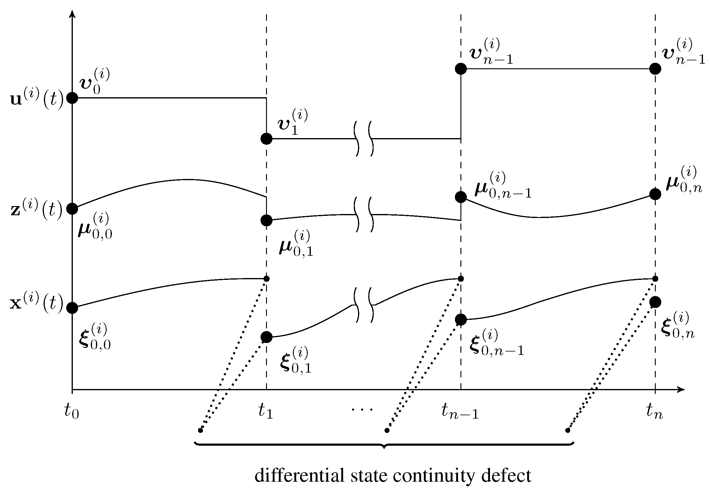
3.1. Multi-Period Multiple-Shooting Discretization

The multi-period multiple-shooting approach discretizes a continuous non-linear uncertain dynamic optimization formulation to an algebraic non-linear program (NLP) with an embedded DAE model within the constraints. The technique entails introducing new optimization parameters ( ξ 0 , j ( i ) , μ 0 , j ( i ) ) for all periods/scenarios i to represent the differential and algebraic state variable initial conditions at the beginning of each shooting interval j, hence the zero subscript, and new equality constraints to remove the discrepancy or defect between the differential state variable values at the final time from the previous interval and the initial time in the current interval.
This idea is sketched in Figure 1 for scenario realization i, where we assume that the time intervals used in the input control trajectory parameterization (i.e., parameterized by the υ j ( i ) ) correspond directly to the defined shooting grid. Our current approach has been to use a rather straight-forward implementation of the multiple-shooting technique, whereby we provide the discretized formulation in full space to an existing sparse NLP solver, as opposed to exploiting the structure of the formulation by implementing a custom (possibly reduced-space) non-linear programming technique (cf. the SCPgen code generation solver within CasADi [24] or the non-linear optimal control solver MUSCOD-II, which uses a tailored reduced SQP algorithm [25]).
Figure 1. Multi-period multiple-shooting discretization.
Processes 03 00541 g001
A general multi-period dynamic optimization formulation that utilizes the multiple-shooting discretization applicable to semi-explicit differential-algebraic equation models can be written as,
min w , d , p J : = ϕ 0 ( p , t n ) + i = 1 n s w i · ϕ i ( ξ 0 , n ( i ) , μ 0 , n ( i ) , d ( i ) , p , θ ( i ) , t n ) st: x ˙ ( i ) ( t ) = f d ( x ( i ) ( t ) , z ( i ) ( t ) , U ( t , υ j ( i ) ) , d ( i ) , p , θ ( i ) , t ) 0 = f a ( x ( i ) ( t ) , z ( i ) ( t ) , U ( t , υ j ( i ) ) , d ( i ) , p , θ ( i ) , t ) ϑ ( γ j ( i ) , t ) 0 = h 0 ( U ( t 0 , υ 0 ( i ) ) , d ( i ) , p , θ ( i ) , t 0 ) ξ 0 , 0 ( i ) x ( i ) ( t j + 1 ; ξ 0 , j ( i ) , μ 0 , j ( i ) , υ j ( i ) , d ( i ) , p , θ ( i ) ) ξ 0 , j + 1 ( i ) = 0 f a ( ξ 0 , k ( i ) , μ 0 , k ( i ) , U ( t k , υ k ( i ) ) , d ( i ) , p , θ ( i ) , t k ) = 0 g ( ξ 0 , k ( i ) , μ 0 , k ( i ) , U ( t k , υ k ( i ) ) , d ( i ) , p , θ ( i ) , t k ) 0 t I i , j , j = 0 , , n 1 k = 0 , , n , i = 1 , , n s w [ w L , w U ] , d [ d L , d U ] , p [ p L , p U ]
In the above formulation, j = 0 , , n 1 represents n shooting intervals. The optimization parameters are partitioned into scenario-independent parameters p , scenario-dependent parameters d = { d ( i ) } i = 1 n s R n d n s and shooting node parameters for differential/algebraic states and input variable parameters, defined collectively as w = ( ξ 0 , 0 ( 1 ) , μ 0 , 0 ( 1 ) , υ 0 ( 1 ) , , ξ 0 , n ( n s ) , μ 0 , n ( n s ) ) R ( ( n x + n z ) ( n + 1 ) + n υ n ) n s , for all shooting nodes and scenario realizations. The continuous control input vector can be defined using a parameterized function u ( i ) ( t ) = U ( t , υ j ( i ) ) based on a piecewise approximation within each shooting interval I i , j , where υ j ( i ) R n υ represent local polynomial coefficients. Note that υ n ( i ) is used in defining the final end point constraint in Problem P2 for notational simplicity, where υ n ( i ) = υ n 1 ( i ) , and can be removed from the NLP (see Figure 1 for a sketch of the parameterization). Additionally, we consider here a fixed end-time formulation where the objective function is represented in Mayer form, which typically only directly depends on the final model states ξ 0 , n ( i ) , μ 0 , n ( i ) , parameters d ( i ) and p and, possibly, the final time t n . The relaxed DAE model, F ( · ) = { [ x ˙ ( i ) ( t ) f d ( · ) ] , [ f a ( · ) ϑ ( γ j ( i ) , t ) ] } , is embedded within the NLP function evaluations and is solved using an appropriate DAE solver for t I i , j , j = 0 , , n 1 with initial differential state conditions x ( i ) ( t j ) = ξ 0 , j ( i ) and algebraic state conditions z ( i ) ( t j ) = μ 0 , j ( i ) for all intervals I i , j , where the intervals are effectively decoupled using the new parameters and are thus independent of each other. The particular formulation given here relies on the use of a relaxed form of the DAEs using a so-called relaxation function represented here through the function ϑ ( γ j ( i ) , t ) , where γ j ( i ) = f a ( ξ 0 , j ( i ) , μ 0 , j ( i ) , υ j ( i ) , d ( i ) , p , θ ( i ) , t j ) is functionally dependent on the shooting parameters at node j. This relaxed form also requires the addition of point equality constraints (for the algebraic model equations) in the NLP at each shooting node to ensure that the original model is obtained upon NLP convergence (see [25,26] for a more complete treatment of DAE relaxation). It is worth noting that using the relaxed DAE approach avoids the otherwise necessary DAE initialization problem.
To simplify the formulation and to assist in our presentation, the multiple-shooting continuity equality constraints, including the initial conditions at t 0 , can be defined as,
c 0 , i ( w 0 , i , d i , p ) h 0 ( υ 0 ( i ) , d ( i ) , p , θ ( i ) , t 0 ) ξ 0 , 0 ( i ) = 0 c j + 1 , i ( w j , i , ξ 0 , j + 1 ( i ) , d i , p ) x ( i ) ( t j + 1 ; ξ 0 , j ( i ) , μ 0 , j ( i ) , υ j ( i ) , d ( i ) , p , θ ( i ) ) ξ 0 , j + 1 ( i ) = 0 j = 0 , , n 1 , i = 1 , , n s
where w j , i = ( ξ 0 , j ( i ) , μ 0 , j ( i ) , υ j ( i ) ) R n x + n z + n υ for j = 0 , , n 1 , and at the final shooting note, w n , i = ( ξ 0 , n ( i ) , μ 0 , n ( i ) ) . The algebraic consistency equality constraints and remaining inequality constraints represent NLP point constraints and can be defined at each shooting node according to,
q j , i ( w j , i , d i , p ) f a ( w j , i , d ( i ) , p , θ ( i ) ) , g ( w j , i , d ( i ) , p , θ ( i ) ) q n , i ( υ n 1 ( i ) , w n , i , d i , p ) f a ( υ n 1 ( i ) , w n , i , d ( i ) , p , θ ( i ) ) , g ( υ n 1 ( i ) , w n , i , d ( i ) , p , θ ( i ) ) j = 0 , , n 1 , i = 1 , , n s
The combined constraint vector for each period/scenario can now be stated as,
c i ( w i , d i , p ) : = c 0 , i ( w 0 , i , d i , p ) q 0 , i ( w 0 , i , d i , p ) , c 1 , i ( w 0 , i , ξ 0 , 1 ( i ) , d i , p ) q j , i ( w j , i , d i , p ) , c j + 1 , i ( w j , i , ξ 0 , j + 1 ( i ) , d i , p ) q n 1 , i ( w n 1 , i , d i , p ) , c n , i ( w n 1 , i , ξ 0 , n ( i ) , d i , p ) q n , i ( υ n 1 ( i ) , w n , i , d i , p ) , i = 1 , , n s
The fully-discretized combined multi-period multiple-shooting NLP formulation of Problem P2 can now be stated in parameterized form according to Problem P3.
min w , d , p J : = ϕ 0 ( p ) + i = 1 n s w i · ϕ i ( w n , i , d i , p ) st: c i L c i ( w i , d i , p ) c i U i = 1 , , n s w : = ( w 1 , , w n s ) [ w L , w U ] d [ d L , d U ] , p [ p L , p U ]
Depending on the constraint type (equality or inequality), the vectors c i L and c i U are appropriately defined. For each scenario i, the concatenated shooting node parameters are defined as w i = ( w 0 , i , , w n , i ) R ( n x + n z ) ( n + 1 ) + n υ n . Note that the embedded DAE model F ( · ) is removed from the NLP formulation, as it is solved using an embedded DAE solver in order to construct the shooting node continuity constraints.
The multiple-shooting approach benefits from a naturally decoupled temporal domain structure that does not require any additional decomposition techniques. This decoupling of each shooting interval is induced by the introduction of the optimization parameters ξ 0 , j ( i ) , μ 0 , j ( i ) for j = 0 , , n 1 and i = 1 , , n s and allows the embedded DAE in each shooting interval and scenario realization to be independently solved in parallel. Accordingly, all scenario realizations i and shooting intervals j over the entire time horizon result in m = n · n s independent integration tasks, which can be broken up and solved in parallel using several processors.

3.2. First-Order Derivative Generation

Shooting-based dynamic optimization approaches necessitate the use of DAE parameter sensitivity in order to generate derivatives of constraints involving implicit functionals. For example, a relaxed semi-explicit index-one parameterized DAE system can be stated as,
x ˙ ( i ) ( t ) f d ( x ( i ) ( t ) , z ( i ) ( t ) , y j , i , t ) = 0 n x f a ( x ( i ) ( t ) , z ( i ) ( t ) , y j , i , t ) ϑ ( γ j ( i ) , t ) = 0 n z t [ t j , t j + 1 ]
x ( i ) ( t j ) = ξ 0 , j ( i )
where all time-invariant parameters within each interval j and scenario i are denoted by y j , i = { ξ 0 , j ( i ) , μ 0 , j ( i ) , υ j ( i ) , d i , p } . From this system, the linear first-order forward sensitivity equations can be derived (in matrix form) as,
s ˙ d ( i ) ( t ) f d x ( t ) s d ( i ) ( t ) + f d z ( t ) s a ( i ) ( t ) + f d y ( t ) = 0 n x × n y f a x ( t ) s d ( i ) ( t ) + f a z ( t ) s a ( i ) ( t ) + f a y ( t ) y ϑ ( γ j ( i ) , t ) = 0 n z × n y t [ t j , t j + 1 ]
s d ( i ) ( t j ) = [ I n x | 0 n x × ( n y n x ) ]
where s { d , a } ( i ) ( t ) = { x ( i ) ( t ) , z ( i ) ( t ) } / y j , i represents differential and algebraic sensitivity variables, respectively, and f { d , a } { x , z , y } ( t ) = f { d , a } ( x ( i ) ( t ) , z ( i ) ( t ) , y j , i , t ) / { x ( i ) ( t ) , z ( i ) ( t ) , y j , i } are Jacobian matrices of the DAE model with respect to the differential variables, algebraic variables and parameters. This extended linear DAE system is solved forward in time alongside the original system to generate s { d , a } ( i ) ( t j + 1 ) , which are used to construct the block structured continuity constraint Jacobian (see, [12]). Particularly efficient techniques and software tools to solve the combined systems of Equations (4) and (6) are discussed by Maly and Petzold [27], Feehery et al. [28], Schlegel et al. [29] and Kristensen et al. [30].

3.3. Second-Order Derivative Generation

Sequential quadratic programming (SQP) algorithms (e.g., filterSQP) or primal-dual non-linear interior-point methods (IPM) (e.g., IPOPT, KNITRO) can often utilize second-order derivatives of the objective/constraint functions, which are used to construct the Lagrangian Hessian (used in the QP subproblem or primal-dual search direction linear solve). To provide such information when using embedded DAE models (i.e., implicit functionals) requires that a second-order sensitivity analysis be performed to construct an approximate representation of the continuity constraint Hessian. All other contributing portions of the Lagrangian Hessian (i.e., explicit objective and point constraint functionals) can be computed exactly using automatic differentiation. A question that arises, and that we seek to address, is whether supplying the second-order derivatives via sensitivity analysis can reduce the number of non-linear programming algorithm iterations sufficiently to justify the additional computation work of second-order sensitivity analysis.
The complete Lagrangian Hessian for our particular multi-period formulation can be stated as,
H ( x , ν ) = x x 2 J ( x ) + i = 1 n s j = 0 n s = 1 n x ν s , j , i c x x 2 c s , j , i ( x ) + l = 1 n q ν l , j , i q x x 2 q l , j , i ( x )
where the italicized symbol x represents a composite vector of all primal NLP variables (as distinct from the model states given by x ( t ) ) and ν = { ν s , j , i c , ν l , j , i q } is a similar concatenation of all dual variables. More specifically, ν s , j , i c are equality constraint multipliers related to the continuity constraints in Equation (1), represented individually here by c s , j , i ( x ) , and ν l , j , i q are either equality or inequality constraint multipliers related to the point constraints in Equation (2), which are again defined individually as q l , j , i ( x ) . In order to compute the individual Hessian portions related to the continuity constraints, ν s , j , i c x x 2 c s , j , i ( x ) , a direct second-order sensitivity analysis can be performed on the portion of the Lagrangian involving the embedded functionals. For example, consider the continuity constraint Lagrangian portion as,
L c ( x , ν c ) = i = 1 n s ν 0 , i c c 0 , i ( y 0 , i ) + i = 1 n s j = 0 n 1 ν j + 1 , i c c j + 1 , i ( x ( i ) ( t j + 1 ; y j , i ) , y j + 1 , i )
where the second portion of this term can be taken as a scalar point-wise implicit functional for each scenario and shooting interval and defined accordingly as,
g j + 1 , i ( y j , i ) = ν j + 1 , i c c j + 1 , i ( x ( i ) ( t j + 1 ; y j , i ) , y j + 1 , i )
Using the sensitivity generation approach described by Ozyurt and Barton [31], the directional Hessian of this point-wise functional can be determined using a forward-over-adjoint direct second-order sensitivity analysis. The particular purpose in this paper is to investigate the application of this technique in the context of a multi-period multiple-shooting algorithm. Furthermore, the application considered in Section 4.1 is in the form an ODE; thus, we restrict our presentation of second-order sensitivity analysis to the purely ODE case. Accordingly, we consider the ODE system given by,
x ˙ ( i ) ( t ) = f ( x ( i ) ( t ) , y j , i , t ) t [ t j , t j + 1 ]
x ( i ) ( t j ) = ξ 0 , j ( i )
For the more general semi-explicit index-one DAE case, we refer readers to the work by Cao et al. [32] for first-order methods, Hannemann-Tamas [33] for higher order methods and Albersmeyer [34] for higher order relaxed DAE methods. The final form of the directional Hessian of a point-wise functional, in the context of our multi-period approach, can be stated as,
2 g j + 1 , i y j , i 2 u = ( λ ( i ) ( t j ) I n y ) x y y ( i ) ( t j ) u + x y ( i ) ( t j ) μ ( i ) ( t j ) + g y y ( t j + 1 ) u + g y x ( t j + 1 ) s ( i ) ( t j + 1 ) q ( i ) ( t j )
where ⊗ represents the Kronecker product; λ ( i ) ( t j ) R n x is a vector of first-order adjoint variables at tj for scenario i; μ ( i ) ( t j ) λ y ( t j ) u R n x is a vector of first-order adjoint variables at tj; s ( i ) ( t j + 1 ) x y ( i ) ( t j + 1 ) u R n x is a vector of directional first-order forward sensitivity variables at t j + 1 (i.e., the solution of directional first-order forward sensitivity equations); q ( i ) ( t j ) R n y ; is a vector of directional second-order adjoint quadrature variables; x y y ( i ) ( t j ) u 0 n x n y is a vector of directional second-order forward sensitivity variables initially known at tj, while x y ( i ) ( t j ) [ I n x | 0 n x × ( n y n x ) ] is a matrix of first-order forward sensitivity variables initially known at t j ; g y y ( t j + 1 ) 0 n y × n y and g y x ( t j + 1 ) 0 n y × n x are second-order derivatives of the scalar functional g j + 1 , i evaluated directly at t j + 1 , which for the multiple-shooting continuity constraints, are simply matrices of zeros. In order to determine the first-order and directional second-order adjoint variables, one needs to first solve forward from tj to t j + 1 the first-order forward sensitivity equations to compute the directional sensitivities s ( i ) ( t j + 1 ) and then solve backward from t j + 1 to tj for each direction u e l , l = 1 , , n y , the combined first- and second-order directional adjoint system given by,
λ ˙ ( i ) ( t ) = f x ( t ) λ ( i ) ( t ) μ ˙ ( i ) ( t ) = f x ( t ) μ ( i ) ( t ) ( λ ( i ) ( t ) I n x ) ( f x y ( t ) u + f x x ( t ) s ( i ) ( t ) ) λ ( i ) ( t j + 1 ) = g x ( t j + 1 ) ν j + 1 , i c μ ( i ) ( t j + 1 ) = g x y ( t j + 1 ) u + g x x ( t j + 1 ) s ( i ) ( t j + 1 ) 0 n x
Additionally, alongside the adjoint system, the quadrature variable vector q ( i ) ( t j ) can be determined from the system,
q ˙ ( i ) ( t ) = f y ( t ) μ ( i ) ( t ) + ( λ ( i ) ( t ) I n y ) ( f y y ( t ) u + f y x ( t ) s ( i ) ( t ) ) , q ( i ) ( t j + 1 ) = 0 n y
where f x ( t ) = f ( x ( i ) , y j , i , t ) / x ( i ) ( t ) R n x × n x  and  f x y ( t ) = 2 f ( x ( i ) , y j , i , t ) / x ( i ) ( t ) y j , i R n x n x × n y in which this latter term is in the form of a stacked Hessian to avoid the otherwise tensor form. Similarly, f x x ( t ) = 2 f ( x ( i ) , y j , i , t ) / x ( i ) ( t ) 2 R n x n x × n x , with all other derivatives defined in an analogous manner. The evaluation of both adjoint and quadrature systems requires the efficient evaluation of several matrix-vector products, comprised of first and second derivative terms, using an appropriate automatic differentiation (AD) tool. Once the adjoint and quadrature variables are determined at tj, the directional Hessian given by Equation (13) can be formed. This process is repeated for all j = 0 , , n 1 and i = 1 , , n s , and the Lagrangian Hessian x x 2 L c ( x , ν c ) is assembled (based on each direction that corresponds to a particular parameter) and further combined with the objective and point constraint Hessian.

3.4. Implementation Details

The results in this paper were generated using a C/C++ implementation, which acts to coordinate the user model input, multi-period multiple-shooting discretization and interaction between several available DAE integration and NLP optimization routines. The implementation utilizes several CSparse routines [35] and interfaces the integration routines CVODES and IDAS from the SUNDIALS suite of solvers [36], the NLP solvers SNOPT [37] and IPOPT [38] and the AD tool ADOL-C [39]. The particular implementation aspect we investigate in this paper is an OpenMP loop parallelization of the high-level DAE integration tasks, and we sketch the approximate solution steps according to Algorithms 1 and 2. Note that the sensitivity generation approach employed by the SUNDIALS integrators follows a so-called “first-differentiate-then-discretize” methodology (i.e., the first- and second-order sensitivity equations are formed prior to applying the discretized numerical integration routine); an alternative approach is a so-called “first-discretize-then-differentiate” technique, whereby certain aspects of the internally-discretized integration algorithm are differentiated either via AD or through numerical differences during the integration procedure. This latter approach is generally known as internal numerical differentiation (IND) and has shown greater solution accuracies and speeds when used in conjunction with embedded model shooting-based dynamic optimization schemes [40,41,42]. Despite the merits of this newer approach, for the ease of availability through existing solvers, we have followed the first approach in this study.
Algorithm 1 Multi-period gradient-based non-linear program (NLP) solution approach with embedded differential-algebraic equations (DAE). QP, quadratic programming.
Input: initial primal and dual variable guesses and tolerances
1: generate scenario realizations: θ = θ ( i ) [ θ L , θ U ] i = 1 , , n s
2: define initial guesses for primal, x [ 0 ] = { w [ 0 ] = { ξ 0 , j ( i ) , μ 0 , j ( i ) , υ j ( i ) } j , i , d [ 0 ] , p [ 0 ] } , and dual variables ν [ 0 ]
3: provide optimality (tol kkt ) and feasibility (tol feas ) tolerances
Output: primal/dual solution x * , ν * to a local minimum of the NLP satisfying tolerances
4: procedure { x * , ν * } NLP_SOLVE( x [ 0 ] , ν [ 0 ] , tol { kkt, feas } )
5:      k 0
6:     initial eval of objective/constraints and 1st derivatives (gradient, Jacobian)
7:      J ( x [ 0 ] ) , x J ( x [ 0 ] )                      ⊳explicit function eval j , i
8:      { c j , i ( x [ 0 ] ) , x c j , i ( x [ 0 ] ) } j , i DAE_SOLVE( x [ 0 ] , θ )                      ⊳implicit function eval j , i
9:      { q j , i ( x [ 0 ] ) , x q j , i ( x [ 0 ] ) } j , i                      ⊳explicit function eval j , i
10:     initial Lagrangian Hessian approximately (or eval exactly via DSOA_SOLVE( x [ 0 ] , ν c [ 0 ] , θ ))
11:     repeat until termination criteria satisfied
12:        check KKTconditions (and other termination criteria)
13:        compute search direction of primal/dual variables ( d x [ k ] , d ν [ k ] ) via QP solver
14:        compute step size α [ k ] via a line search (requires objective/constraint eval)
15:         perform step: x [ k ] x [ k ] + α [ k ] d x [ k ] ν [ k ] ν [ k ] + α [ k ] d ν [ k ]
16:         k k + 1
17:        re-evaluate function derivatives j , i (used to construct the next QP)
            { x c j , i ( x [ k ] ) } j , i DAE_SOLVE( x [ k ] , θ )
            { x q j , i ( x [ k ] ) } j , i
18:        update Hessian approximately (or eval exactly via DSOA_SOLVE( x [ k ] , ν c [ k ] , θ ))
19:     end
20: end procedure
Algorithm 1 sketches a high-level SQP-type solution procedure for the NLP given by Problem P3. The purpose of outlining the NLP solution approach is to provide some insight to where specifically within the algorithm an embedded DAE solver (and possibly a first- and/or second-order sensitivity solution) is required. Alternatively, one could utilize a non-linear interior-point approach where the major differences from Algorithm 1 are an adaptive barrier update strategy that nests a procedure similar to Steps 11 to 18 where the Newton search direction is determined from a single solution of the primal-dual equations as opposed to Step 13 shown here, which solves the QP to optimality (see [43] for the details). For the particular algorithm shown, initially, a complete specification of the scenario realization set, initial primal (and possibly dual) variables and termination tolerances is provided. Note that an initial simulation of the embedded DAE can be used to determine initial feasible guesses for the primal shooting variables ξ 0 , j ( i ) and μ 0 , j ( i ) for all j and i, given υ j ( i ) , d and p . The dual variables can be initialized at zero (cold start) or warm started if a previous similar NLP solution is available. Following this, an iterative quadratic programming procedure is performed whereby: (1) objective, constraint and derivative functions are evaluated; (2) termination criteria are checked (and possibly termination signalled); (3) a search direction is determined from a quadratic program (using either an active-set or primal-dual interior-point method) (this step is often preceded by a dimensionality reduction of the original QP; additionally, infeasible QP’s are handled in a so-called feasibility restoration phase); (4) a globalization procedure is performed to determine the step size (we note a line search, but a trust-region approach within the QP itself is possible); and (5) primal and dual variables are updated and objective, constraint and derivative functions are re-evaluated. The time-dominant aspect of the algorithm occurs with the embedded implicit function evaluations denoted by dae_solve, which we handle specifically within our implementation by Algorithm 2. Additionally, note that during the step size globalization procedure, re-evaluation of objective and constraint functions is required, and for the multiple-shooting continuity constraints, sensitivity generation is deactivated within dae_solve. We remark that an algorithm for the procedure dsoa_solve follows in a similar manner to Algorithm 2, whereby a second-order forward-over-adjoint sensitivity analysis is performed for each shooting interval j and scenario i, which is specifically handled by the SUNDIALS integration solvers.
Algorithm 2 Parallel multi-period DAE and first-order sensitivity function evaluation.
Input: state initial conditions, control parameters and invariant model parameters
1: specified scenario realizations θ = { θ ( i ) } i = 1 n s
2: NLP variables x = { w = { ξ 0 , j ( i ) , μ 0 , j ( i ) , υ j ( i ) } j , i , d, p }
3: provide relative (tol rel ) and absolute (tol abs ) integration tolerances for DAE solution
Output: differential state solution x ( i ) ( t j + 1 ) , s d ( i ) ( t j + 1 ) = x ( i ) ( t j + 1 ) / { w i , d i , p } i , j
4: procedure { x , s d } dae_solve(x, θ, tol { rel, abs } )
5:    for i : = 1 to n s do                 ▹ in parallel using OpenMP for k = 1 , , n · n s tasks
6:       for j : = 0 to n 1 do
7:          set initial differential and algebraic DAE variables:
x ( i ) ( t j ) ξ 0 , j ( i )
z ( i ) ( t j ) μ 0 , j ( i )
8:          set initial differential DAE sensitivity variables:
s d ( i ) ( t j ) [ I n x | 0 n x × ( n y n x ) ]
9:          solve DAE and 1st order sensitivity system
{ x ( i ) ( t j + 1 ) , s d ( i ) ( t j + 1 ) } ← sundials_dae_solver
10:       end for
11:    end for
12: end procedure
Algorithm 2 computes the solution of the discretized relaxed embedded DAE (both state and first-order sensitivity variables over each interval and scenario), which is used to evaluate the continuity constraints and associated Jacobian at each major iteration of the NLP algorithm. Note that using the relaxed DAE approach, the initial conditions of the differential and algebraic states are by formulation always consistent at t j . For each shooting node and scenario realization, the embedded DAE is initialized in Step 7 of Algorithm 2 by the NLP parameters; next, in Step 8, the initial values of the differential sensitivity variables (in matrix form) are set to an augmented identity matrix. The next step is to solve the DAE and first-order sensitivity system using an appropriate DAE solver with efficient methods for handling the sensitivity equation solution. The last step (not shown) is to construct the continuity equations and Jacobian, the latter of which is a matrix with appropriately positioned blocks of sensitivity variables at t j + 1 (see [12]). Several remarks are warranted with respect to Algorithm 2: (1) when using an implicit integration routine, such as IDAS from SUNDIALS, one needs to additionally provide initial values for the time-derivatives of the differential states x ˙ ( i ) ( t j ) , the initial time-derivatives of the differential sensitivity variables s ˙ d ( i ) ( t j ) and the initial algebraic sensitivity variables s a ( i ) ( t j ) ; (2) the differential time-derivatives are determined from a single evaluation of the ODE portion of the DAE; and (3) the differential time-derivative sensitivity variables and algebraic sensitivity variables are computed from a linear solve of the initial sensitivity equations (note that this requires a single initial factorization and several back solves using multiple right-hand-side vectors for a linear system given by A X = B ). We elaborate on this last point. For example, given that variables x ( i ) ( t j ) , z ( i ) ( t j ) , and s d ( i ) ( t j ) are known at t j , we can rearrange the initial first-order sensitivity equation system as,
I n x + + f d z ( t j ) 0 n z × n x f a z ( t j ) s ˙ d ( i ) ( t j ) s a ( i ) ( t j ) = f d x ( t j ) s d ( i ) ( t j ) + f d y ( t j ) + y ϑ ( γ j ( i ) , t j ) f a x ( t j ) s d ( i ) ( t j ) f a y ( t j ) + y ϑ ( γ j ( i ) , t j )
and solve for the initial values of s ˙ d ( i ) ( t j ) and s a ( i ) ( t j ) (in matrix form).
The particular details of the underlying ODE/DAE or NLP solution used in this paper can be found in the previously noted references. However, we remark on the following: both first- and second-order sensitivity analysis is handled directly by the SUNDIALS integrators, and all the user needs is an appropriate AD tool to form Equations (6) and (13) to (15); for our implementation, we used the tape-based features of ADOL-C for all serial computation and the tapeless forward differentiation features when evaluation is needed within parallel OpenMP regions of the code (we refer readers to the ADOL-C manual for the particular details of tapeless and tape-based operator overloaded AD). We further note that all code and third party libraries used for our example problems were compiled using GCC-4.7 (with OpenMP-3.1) and run using 64-bit Linux. The hardware was an HP Proliant computing server configured with four sockets using AMD Opteron 6386SE series chips (16 cores per chip) at 2.8 GHz, which provide a total of 64 available cores (processors/threads). Furthermore, an appropriate amount of memory was allocated/utilized to suit the requirements of the program.

4. Example Problems

We demonstrate our proposed parallel multi-period dynamic optimization approach using a batch reactor problem and a large-scale air separation problem. The objective is to assess the computational performance (resource utilization efficiency and scalability) of the proposed method when the number of scenarios and shooting intervals (embedded integration tasks), model size and available computing processors are increased.

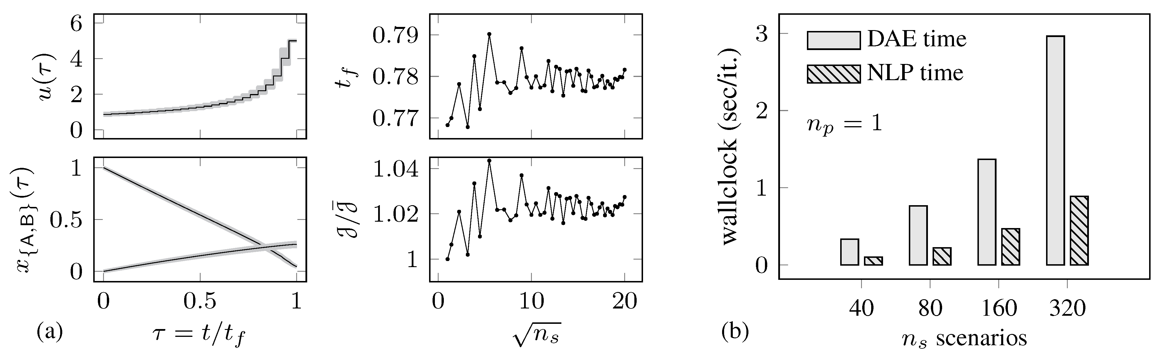
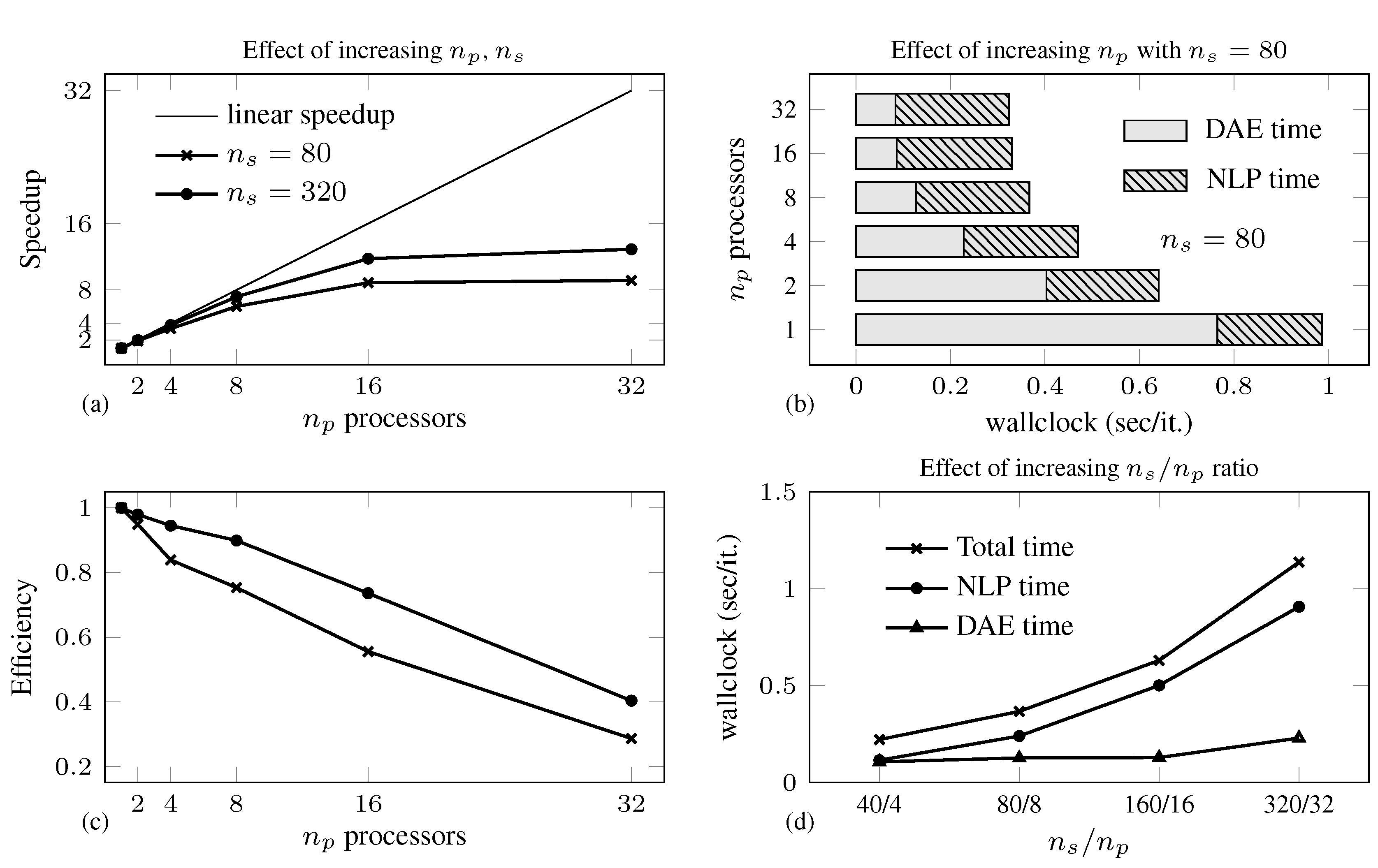
4.1. Batch Reactor Problem

The initial portion of this example is performed with a parallel implementation using the ODE integration solver CVODES and NLP solver SNOPT. Subsequently, further comparison is made using second-order sensitivity analysis for generating the Lagrangian Hessian when using the NLP solver IPOPT with the exact Hessian versus an approximate limited memory quasi-Newton update, which only requires first-order sensitivity information. For this last portion, we currently only report serial solution times of the implementation.
The case study example considered is adapted from [16] and involves a batch reactor problem in a purely ODE form that follows a first order reaction scheme A B , where the kinetic parameters are assumed to be uncertain. The objective is to operate the reactor for an indeterminate duration (i.e., design variable), such that a maximum profit is achieved. The objective function comprises a revenue term proportional to the product conversion, x B , and an operating cost dependent on the duration of operation t f . The optimization problem is defined according to Formulation E1,
min t f , u ( i ) ( τ ) i J : = c 1 t f 0 c 2 i = 1 n s w i c 0 x B ( i ) ( 1 ) st: x ˙ A ( i ) ( τ ) = [ θ 1 ( i ) u ( i ) ( τ ) θ 2 ( i ) + u ( i ) ( τ ) ] x A ( i ) ( τ ) t f x ˙ B ( i ) ( τ ) = θ 1 ( i ) u ( i ) ( τ ) x A ( τ ) t f x { A , B } ( i ) ( 0 ) = x { A 0 , B 0 } x { A , B } ( i ) ( τ ) [ 0 , 1 ] u ( i ) ( τ ) [ 0 , 5 ] , τ [ 0 , 1 ] , i = 1 , , n s θ 1 ( 0 . 45 , 0 . 55 ) , θ 2 ( 2 . 15 , 2 . 25 )
The initial state conditions are taken as x A 0 = 1 , x B 0 = 0 i , where we use a normalized time horizon, such that the end-time t f is taken as a design parameter. The cost/objective coefficients are set as c 0 = 700 , c 1 = 50 , c 2 = 2 ; and the weights are set as w i = 1 / n s . The parameterized control profile is taken to be piecewise constant, and initial guesses for the polynomial coefficients are set to 1.0 for all scenarios and shooting intervals. For this example, we kept the number of shooting intervals constant at n = 25 and with a uniform size over the time horizon. The uncertain model parameters ( θ 1 , θ 2 ) were determined by sampling uniformly between the defined bounds.
Figure 2 depicts a base line solution to formulation E1 using a single processor with increasing scenario realizations. For the input and state solution trajectories in Figure 2a, the solid input and state trajectory lines represent the nominal solution, while the shaded bands represent an envelope of possible solutions generated via discrete realizations of the uncertain parameter values. Interesting aspects to note include: (1) as the number of scenarios is increased, both the optimal objective value (defined here as the ratio of the multi-period objective value to the nominal objective value, J / J ¯ ) and parametric degree of freedom, t f , converge to a point (or rather confidence interval), which can be considered close to the true solution of the original infinitely dimensional stochastic program; and (2) considering n s = 40 as the base line, we see a ×2.26, ×4.20, ×8.81 increase in total computation time per major SQP iteration for n s = 80 , 160 , 320 , respectively (i.e., almost a linear increase in computation time as scenario realizations are added). Based on Figure 2a, an appropriate number of scenarios to use would exceed 80, where the profiles for J / J ¯ and t f level off.
Figure 2. Case Study 1: (a) control input and state trajectories (nominal solution represented by the solid line) and (b) base line DAE and NLP solution times for increasing n s .
Processes 03 00541 g002
Parallel solution times for the total program are reported in Table 1 for n s = 40 , 80 , 160 , 320 (number of scenario realizations) and n p = 4 , 8 , 16 , 32 (number of processors/threads). Additionally, the serial solution time is reported for each scenario realization level and the time required for the nominal dynamic optimization solution (i.e., n s = 1 ). We further remark that the parallel solution times are an average of three independent experiments; the NLP problem dimension is represented by the total number of variables vars and equality/inequality constraints cons; and the number of NLP iterations until termination is given by iter. Considering n s = 80 as the ideal number of scenarios to use, we see a × 116 total computation increase from the nominal solution, and if 16 processors are used (i.e., the maximum advisable n p for the given problem size; see the discussion below), this number drops by 66%, indicating a × 39 increase from the nominal serial solution. Given that we are only parallelizing the discretized implicit DAE integration tasks, a 66% improvement is a promising result. A breakdown of the specific computation performance using speed-up S = T serial / T parallel , where T serial and T parallel represent serial and parallel program run times, respectively, and efficiency E = S / n p , is sketched in Figure 3. Note, for our particular case that we consider each metric to be based on the time to evaluate objective/constraint functionals and derivatives (denoted as DAE time) and exclude the serial in-solver time related to the matrix computations within the NLP solver (denoted as NLP time). From Figure 3a, the parallel performance in terms of speed-up is quite good up to about eight processors/threads, after which a significant deviation from ideal speed-up is observed. This undesirable behaviour using n p 16 , for our chosen problem size of m = n · n s , can be explained using the laws of Amdahl and Gustafson [44]. Amdahl’s law gives us an indication of the possible scalability or maximum speed-up for a fixed problem size, while Gustafson’s law can be used to understand the influence of problem size on scalability. Considering first Amdahl’s law, the parallel time can be approximated as T parallel : = f T serial + ( 1 f ) T serial / n p , where f represents an inherent serial fraction of the overall computation, which results in the speed-up expression S ( n p ) = ( f + ( 1 f ) / n p ) 1 , and as n p , the maximum possible speed-up is S ( ) = f 1 . Therefore, for our particular example, if the time to evaluate the NLP objective/constraint functionals has an inherent serial portion of 10%, then we would achieve a maximum possible speed-up of 10. Fortunately, if we further consider the influence of problem size m, whereby the serial fraction of the program is now considered a function of problem size f ( m ) , it can be shown using Gustafson’s law that speed-up can be given by S ( m , n p ) = f ( m ) + n p ( 1 f ( m ) ) , where f ( m ) : = a ( m ) / ( a ( m ) + b ( m ) ) , and a ( m ) and b ( m ) represent the inherent serial and parallel portions, respectively. Thus, if we are able to better load the processors with more work such that the inherent serial portion diminishes relative to each parallel portion ( b ( m ) a ( m ) ), then the fraction f ( m ) decreases with increasing m, and as m , the speed-up will approach n p . This concept can be better seen using the log-p model where T parallel : = T serial / n p + log 2 ( n p ) and T serial m (see p. 79 of [44]). The speed-up expression can be derived as S ( m , n p ) = n p / ( 1 + ( n p / m ) log 2 ( n p ) ) , and if m = M n p where M is the work per processor, then the speed-up (and efficiency) can be controlled by limiting the influence of the log 2 ( n p ) term by increasing M. Additionally, to ensure a uniform M on each processor, one needs to properly balance and schedule the distribution of work. For example, in our case study, we found that if the computation time on each processor for a chunk size of M is relatively constant between processors, then a so-called OpenMP static scheduling policy is adequate, while if the computation time differs, a dynamic (round-robin) policy is preferred, which is able to better balance the computation load between processors. To achieve good scalability, one often tries to keep the efficiency fixed by increasing the problem size (or rather, work per process, M) at the same rate as the number of processors/threads n p . If this is possible, then the algorithm can be considered weakly scalable; on the other hand, if one is able to keep the efficiency constant for a fixed problem size as n p increases, then the algorithm is considered strongly scalable. Based on these definitions of scalability, our particular parallel implementation is not strongly scalable; however, there is enough evidence to suggest weak scalability. For example, from Figure 3d, the “DAE time” (i.e., out-of-solver NLP function evaluation time of which the majority represents the parallelized DAE solution) remains relatively constant for a work load of M = 250 integration tasks per processor up to about n p = 16 after which a slight increase in wall-clock time is observed (i.e., decrease in efficiency), which can be attributed to a greater influence of parallel computation overhead (i.e., the previously noted log 2 ( n p ) term) relative to the chosen computation load M.
Table 1. Case Study 1: parallel computation results comparing increasing n s .
Total Program Solution Time (s)
n s m varsconsiter J / 100 t f n p = 1 n p = 4 n p = 8 n p = 16 n p = 32
125785324 (60)−1.49110.76830.3890.2510.2350.201
4010003081208140 (1239)−1.52350.778517.488.877.016.266.24
8020006161416146 (2244)−1.54630.786845.4121.6116.8815.2014.87
160400012,321832149 (4395)−1.53400.782390.0042.3734.7430.8730.35
320800024,64116,64149 (8718)−1.52000.7772188.6982.6065.1056.7455.67
m = n · n s , total No. integration tasks, where n = 25 ; SNOPT solver with No. minor QP iter.in brackets; NLP optimality/feasibility tol. = 1 × 10 6 , 1 × 10 8 , DAE relative/absolute tol. = 1 × 10 6 , 1 × 10 8 .
Figure 3. Case Study 1: speed-up, efficiency and wall-clock times for increasing n s .
Processes 03 00541 g003
The next aspect of the study considers assessing the use of forward-over-adjoint second-order sensitivity analysis in order to form a representation of the Lagrangian Hessian. Note, that such a procedure is quite expensive given the numerous forward and reverse sweeps of the integrator for all shooting intervals and scenarios, and the objective here is to provide some insight on the additional cost when compared to a quasi-Newton approximation scheme. For demonstration purposes, we use the interior-point non-linear programming solver IPOPT-3.11.9 with default options and MA27, MC19 for the linear solver and scaling, respectively. Results comparing the limited memory BFGS approximation to the sensitivity approach are reported in Table 2, where we highlight the total number of primal-dual IPM iterations, total computation time, time spent in the NLP solver, total time to compute the continuity constraint Jacobian using forward sensitivity analysis and additional point constraint first derivatives using AD, which we denote overall as FSA, and total time to compute the lower triangular portion of the Lagrangian Hessian (Equation (8)) via second-order sensitivity analysis (including all AD computations), which we denote as DSOA. From Table 2, comparing columns qn and ex for quasi-Newton and exact Hessian, respectively, we make the following observations: the DSOA approach reduces the overall number of primal-dual iterations (as one would expect); the total computation time increases on average by about × 25 over the quasi-Newton approach where about 98% of the total computation is spent generating the Lagrangian Hessian. From these results, it is quite clear that providing the Lagrangian Hessian of our multi-period NLP formulation by means of second-order sensitivity analysis is very expensive. From an implementation perspective, the computation in each shooting interval could be parallelized; however, this is unlikely to lead to a significant enough decrease in time to justify the use of second-order sensitivities as implemented in our study. An alternative approach proposed by Hannemann and Marquardt [45] is to use a so-called composite or aggregated approach, which only requires a single second-order sensitivity computation encompassing all shooting intervals. Such a technique has been shown to reduce the Hessian computation time considerably when used in the context of implicit Runge–Kutta integration techniques. Given our adherence to the SUNDIALS solvers in this work, we have not explored this new technique, but it would be the next logical step.
Table 2. Case Study 1: serial computation results comparing Hessian generation approach.
iterTotal (s)NLP (s)FSA(s)DSOA(s)
n s J / 100 qnexqnexqnexqnexex
1−1.4911 p52480.79322.960.3110.1110.4820.29722.56
40−1.5235 p706627.81632.422.2770.59125.5412.27619.56
80−1.5463 p656448.611218.463.6971.06044.9123.571193.82
160−1.5340 p7165107.32204.618.0231.92099.3247.122155.57
320−1.5200 p4944151.24397.6411.703.962139.592.784300.90
IPOPT optimality tolerance = 1 × 10 6 .

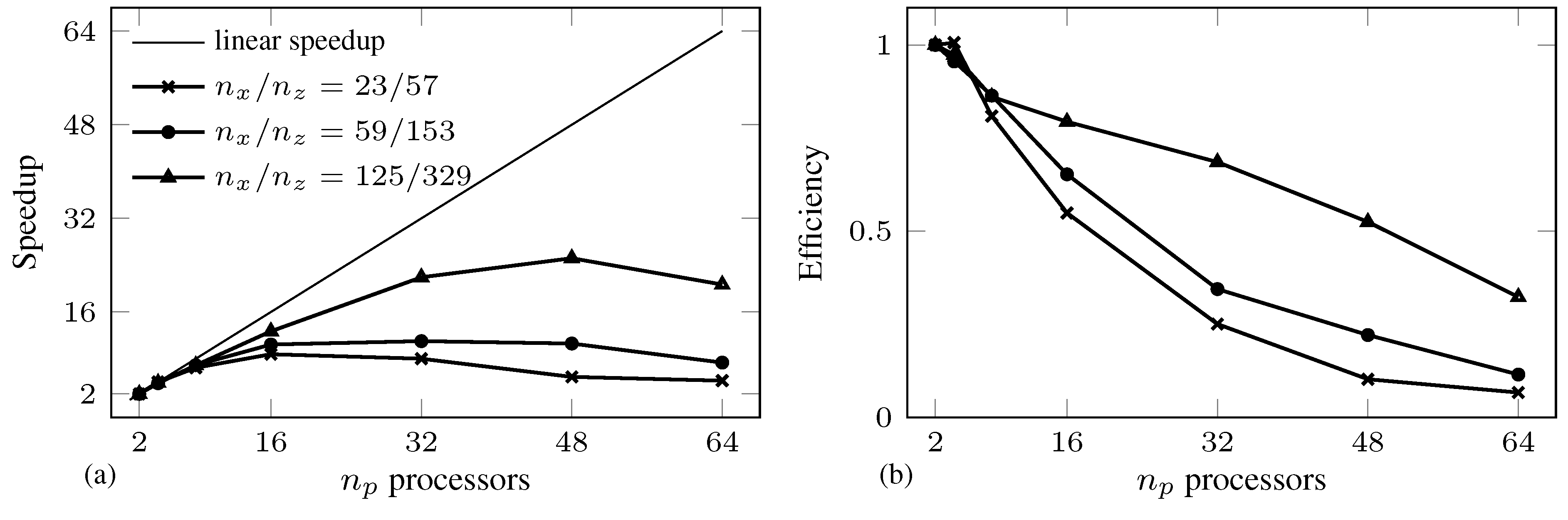
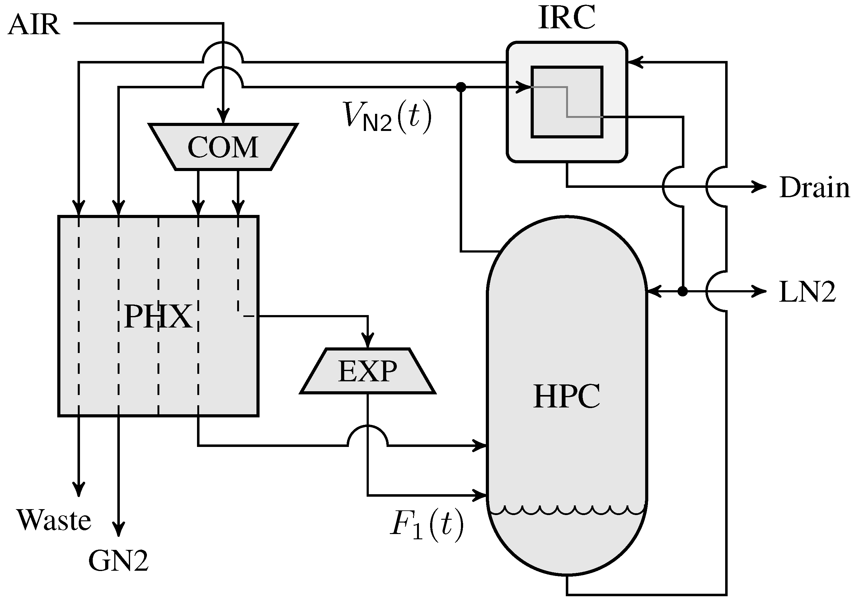
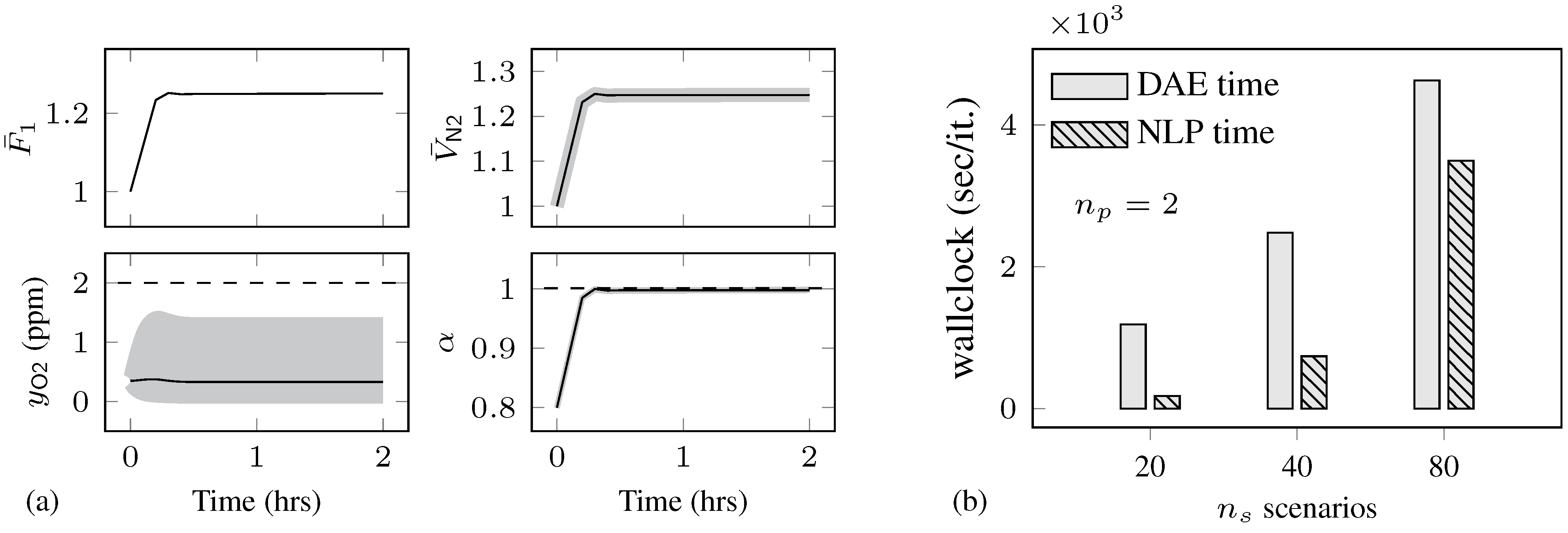
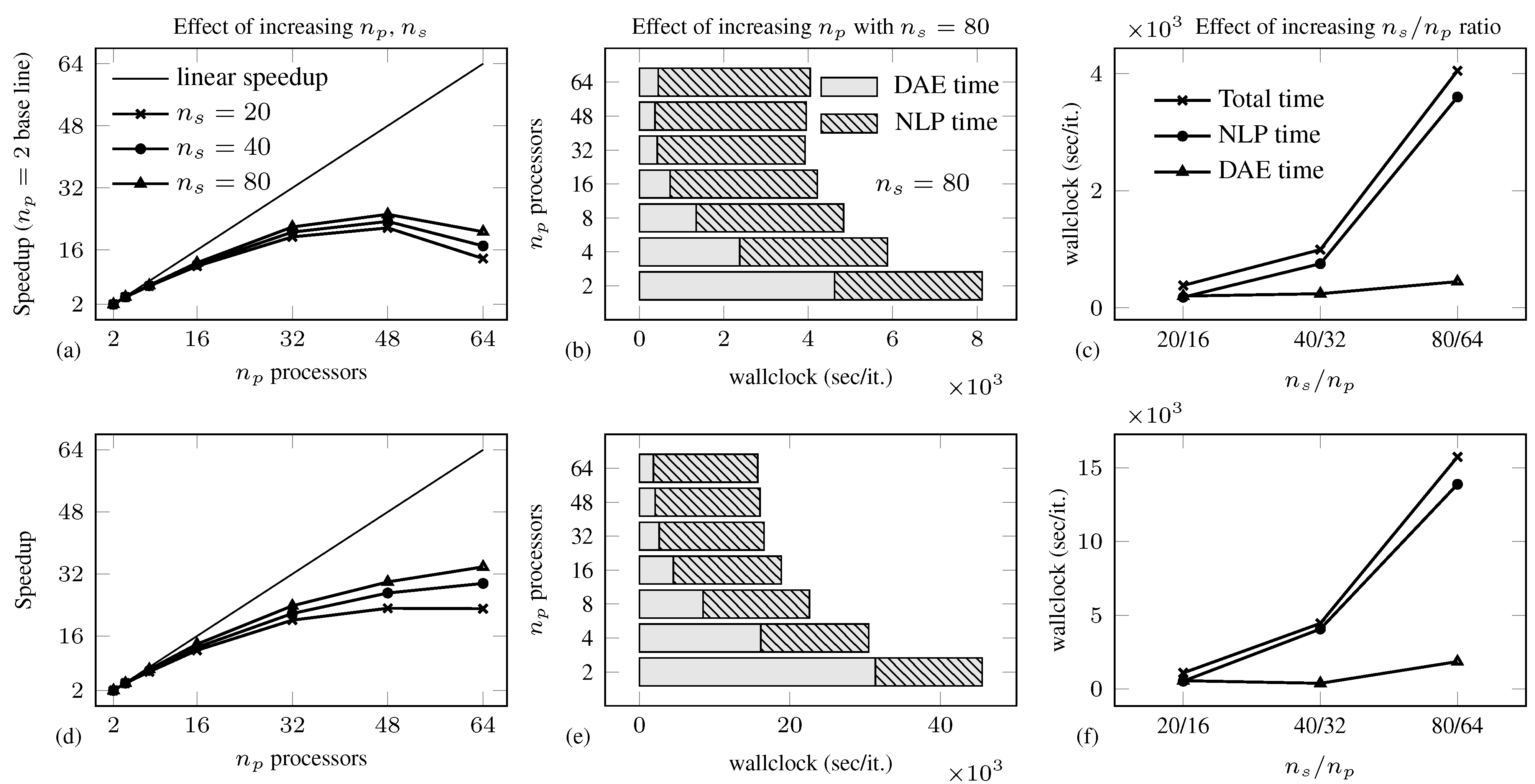
4.2. Air Separation Problem

This next case study explores further the influence of processor loading on algorithm scalability and additionally the influence of DAE model size. A large-scale DAE air separation model is used, which considers the separation of nitrogen from air. The model used here was adapted from Cao [46], and a simplified process schematic is shown in Figure 4. As a first step, air enters from the atmosphere and is compressed using a multi-staged compressor (COM); impurities are then removed using several adsorption units; high pressure purified air is then cooled in a multi-path heat exchanger (PHX) using the returning gas product (GN2) and waste streams from a high pressure distillation column (HPC); the cooled air stream is then split where a portion goes through a turbine (EXP) to promote further cooling before entering the bottom of the distillation column, while the other stream goes directly to the distillation column. The air entering the column is converted into high purity gaseous nitrogen, which exits at the top, and crude liquid oxygen, which accumulates at the bottom. A portion of the high purity nitrogen gas is drawn off as product ( V N 2 ), while the remainder is fed to an integrated reboiler/condenser (IRC) to exchange heat with a crude oxygen stream, which is drawn from the bottom of the column. The heat exchange converts gaseous nitrogen to liquid, which is then refluxed back to the top of the column and optionally drawn off as liquid nitrogen product (LN2).
The portion of the process we focus on in this study is the distillation column (HPC) and integrated reboiler/condenser (IRC) units, with the air feed to the bottom of the distillation column ( F 1 ) as the input stream. A detailed listing of the variables and equations used in our particular model can be found in [46]. The optimization formulation considered seeks to determine a robust control profile to transition from one steady state to another while satisfying path inequality constraints on product composition (defined in the form of product impurity y O 2 ) and tray flooding (defined implicitly by ensuring the vapour velocity ν n t is below the flooding velocity ν ¯ n t on the critical tray of n t , which represents the top tray of the column), all while under the influence of uncertainty within key model parameters. The formulation can be defined as a continuous multi-period dynamic optimization problem according to the following equations,
min u ( t ) J = i = 1 n s w i t 0 t f y ( i ) ( t ) y sp 2 + Δ u ( t ) 2 d t st: DAE model (125 ODEs, 329 AEs) x ( i ) ( t 0 ) x ss = 0 (initial steady state) V N 2 sp V N 2 ( i ) ( t f ) 0 (min. production rate at t f ) y O 2 ( i ) ( t ) y O 2 max 0 (max. product impurity) ν n t ( i ) ( t ) ν ¯ n t ( i ) ( t ) 0 (avoid tray flooding) u ( t ) [ u L , u U ] , t [ t 0 , t f ] , i = 1 , , n s θ [ θ L , θ U ]
where y ( t ) = V N 2 ( t )  and  y sp = V N 2 sp are the measured output and corresponding final desired set-point for the nitrogen production rate; u ( t ) = F 1 ( t ) is the manipulated input feed rate of air to the first tray (i.e., column bottom); θ = [ η , Δ P ] is a vector of uncertain model parameters, which we select a priori as the tray efficiency η [ 0 . 4 , 0 . 6 ] and pressure drop between trays Δ P [ 0 . 45 , 0 . 55 ] kPa. Note the stated DAE model dimension of n x = 125 differential and n z = 329 algebraic variables/equations excludes all sub-expression algebraic variables/equations; thus, the algebraic portion of the model is in fact quite larger than it might appear. Select output and state solution trajectories of Formulation E2 are plotted in Figure 5 for variables F ¯ 1 ( t ) F 1 ( t ) / F 1 ( t 0 )  and  V ¯ N 2 ( t ) V N 2 ( t ) / V N 2 ( t 0 ) and path constrained variables y O 2 ( t )  and  α ( t ) , where  α ( t ) = ν n t ( t ) / ν ¯ n t ( t ) 1 .
Figure 4. Case Study 2: air separation process schematic.
Processes 03 00541 g004
Figure 5. Case Study 2: (a) robust control and select output trajectories (nominal solution represented by the solid line) and (b) base line DAE and NLP solution times for increasing n s .
Processes 03 00541 g005
A piecewise linear input control profile was selected, and the rate of change of this profile was penalized in the optimization objective function. Note that in order to prevent unnecessary chattering of the control input in the latter portion of the time horizon, the profile uses an evenly-distributed parameterization of n 1 shooting intervals within the first 0.5 h of the time horizon and a final single interval within the remaining 1.5 h. From Figure 5, we see that the production rate of nitrogen vapour V ¯ N 2 ( t ) and the vapour velocity ratio α ( t ) both increase in proportion to the feed air input F ¯ 1 ( t ) (as one would logically expect); however, due to the flooding constraint, there is a clear limitation on the rate of production increase, and the influence of parametric uncertainty within the model directly affects the onset of constraint activation. Ultimately, we are able to establish an optimal control profile that is robust to the prescribed uncertainties within the model and adherent to the constraints within the formulation. In order to establish a performance base line, we consider a fixed number of shooting intervals, three increasing scenario sizes and two processors. For shooting intervals n = 6 and scenarios n s = 20 , 40 , 80 , the average total solution time per major SQP iteration was approximately 1 . 37 × 10 3 s (22.7 min), 3 . 22 × 10 3 s (53.6 min) and 8 . 12 × 10 3 s (135.4 min), respectively; which are about ×15.53, ×36.68 and ×92.51greater than the nominal solution time of 1.46 min. The corresponding ratio of time spent in the NLP solver versus the DAE solver was 0.14, 0.30 and 0.88, respectively, which indicates that as the problem size increases, the computational burden shifts dramatically from the DAE solver to the in-solver aspects of the NLP solver (e.g., active-set determination, matrix factorizations, matrix-matrix/matrix-vector multiplications, etc.)
With the base line solution properties established, we now turn to assessing the potential computation speed-up via our parallel multi-period approach. Table 3 lists the optimization problem size and solution results, in terms of the number of SQP iterations and total wall-clock times, for an incremental number of integration tasks m = n · n s (where n = { 6 , 12 } and n s = { 20 , 40 , 80 } ) using an increasing number of computing processors. Considering first a problem with n = 6 and increasing scenario realizations ( n s = { 20 , 40 , 80 } ), we observed good scaling properties using at most n p 32 . For example, using n p = 16 , we observe an overall average computation speed-up of ×3.57, ×2.88, ×1.93 for each n s , respectively; and for n p = 32 , ×4.54, ×3.24, ×2.07, where the decrease in rate of speed-up from 16 to 32 processors is due to the increasing serial portion of the NLP solver. If we remove this large serial NLP portion, it can be confirmed that the parallel implementation of the embedded DAE shooting intervals can be done fairly efficiently. For example, Figure 6a provides speed-up trends for n p from two to 64 at a fixed amount of work (m) based on the so-called “DAE time” as defined in the previous case study. It is evident that good, strong scaling properties are observed up to about 32 processors, after which a more sharply decreasing rate is observed, which can be attributed in part to an insufficient work load per processor M. Figure 6b compares the amount of time, per major SQP iteration, spent in the DAE solver versus the NLP solver. Considering a problem size of m = 480 and imposing an increase in processors from two to 64, we see a significant reduction in DAE solution time relative to the serial NLP solution time. Furthermore, from Figure 6c, if we increase the number of processors in proportion to the problem size m, the DAE solution time remains relatively constant, which indicates reasonably good weak-scaling properties. For the case of n = 12 (see Figure 6d,e), where we effectively double the NLP size, better speed-up with increasing number of processors is observed, which indicates the expected result that as we increase the work per processor (M), we also reduce the relative parallel overhead and ultimately see better, strong scaling properties. However, for the particular active-set SQP solver used in this study, we quickly run into significant serial computation overhead within the QP subproblems (i.e., a sharp increase in the number of QP iterates).
Finally, we consider the aspect of increasing the embedded DAE size and provide a relative comparison on the influence of DAE size on the overall parallel scalability of the implementation. Table 4 compares model sizes of n x / n z = { 23 / 57 , 59 / 153 , 125 / 329 } where n x and n z represent the number of differential and algebraic state variables, respectively, that are a result of increasing the number of distillation column trays according to n t = { 5 , 17 , 39 } . The base line total solution time per SQP iteration for each model size using n s = 80 scenarios was 6.24 min, 20.23 min and 135.37 min, respectively, which are over 100-times the nominal solution time. Through parallelization, these base line times can be reduced by about ×3.6, ×2.4 and ×1.9, respectively; where again, we observe that as the serial NLP portion grows, the potential speed-up diminishes. Figure 7 reveals more closely the speed-up and efficiency excluding the influence of the serial in-solver NLP contribution. As the model size is increased (i.e., more expensive integration tasks), a more pronounced improvement is observed when compared to increasing the number of integration tasks per processor via discretization alone (i.e., increasing M via increasing n s or n). In other words, if one compares the delta in speed-up from n x / n z = 59 / 153 and n x / n z = 125 / 329 in Figure 7a to the delta in speed-up from n s = 40 and n s = 80 in Figure 6a, then a larger deviation results from increasing the model size versus the discretization refinement. This result is particularly positive and highlights that one is able to more easily achieve better parallel scalability using larger embedded DAE models versus creating more independent integration tasks.
Table 3. Case Study 2: parallel computation results comparing increasing n and n s .
Total solution time (s)/ 1 . 0 × 10 5
n n s mvarsconsiter J / 10 n p = 2 n p = 16 n p = 32 n p = 48 n p = 64
616318431949 (1308)1.01590.0079
2012063,68063,97414 (42,704)1.01340.19080.05350.04200.04260.0501
40240127,360127,95516 (85,672)1.01810.51460.17850.15890.15960.1688
80480254,720255,91517 (170,391)1.01561.38080.71660.66690.67200.6882
121125914593012 (3221)1.01410.0135
20240118,280118,80818 (81,273)1.01140.71630.19550.15580.14910.1474
40480236,560237,62811 (162,037)1.01590.91670.51790.48910.47320.4714
80960473,120475,26817 (322,952)1.01297.74683.20472.81562.72392.6748
NLP optimality/feasibility tol. = 1 × 10 4 , 1 × 10 6 , DAE relative/absolute tol. = 1 × 10 3 , 1 × 10 4 .
Figure 6. Case Study 2: speed-up and wall-clock times for increasing n p and n s , where n = 6 fixed for (a) to (c) and n = 12 fixed for (d) to (f).
Processes 03 00541 g006
Table 4. Case Study 2: parallel computation results comparing different DAE dimensions.
Total Solution Time (s)/ 1 . 0 × 10 5
n x / n z * m varsconsiter J / 10 n p = 2 n p = 16 n p = 32 n p = 48 n p = 64
23/57656656819 (184)0.85590.0006
48045,28045,91522 (16,326)0.85600.08240.02300.02470.03680.0416
59/15361490149212 (616)1.01110.0011
480119,200119,83518 (38,928)1.01100.21850.08960.08700.08810.1052
125/32963184319410 (1294)1.01590.0079
480254,720255,91517 (170,391)1.01561.38080.71660.66690.67200.6882
* dimension based on number of distillation trays n t = { 5 , 17 , 39 } ; problem size based on n = 6 and n s = { 1 , 80 } .
Figure 7. Case Study 2: speed-up and efficiency for increasing DAE size n x / n z based on n t = { 5 , 17 , 39 } , with n = 6 , n s = 80 fixed.
Processes 03 00541 g007

5. Concluding Remarks

In this paper, we have presented a parallel computing approach for large-scale dynamic optimization under uncertainty that targets the decomposition of the embedded differential-algebraic equation model. A combined multi-period multiple-shooting approach was used to discretize the DAE optimization formulation to yield a multi-period NLP formulation with embedded implicit DAE functionals within the constraints. The DAE model and sensitivity equations corresponding to each shooting interval and scenario constitute independent integration tasks, well suited for parallel processing. Our multi-period approach was applied to a large-scale DAE air separation model comprising up to 125 ODEs and 329 algebraic equations for the purpose of obtaining a robust optimal control profile subject to uncertainty in the model parameters. Results indicated fairly good parallel scalability using a parallel OpenMP implementation of the DAE solution; however, the extent of scalability depends largely on the amount of work per processor and on the ability to effectively balance the work load between processors. In this paper, we were able to demonstrate the benefits of parallelizing the DAE solution portion of the multiple-shooting algorithm; however, as the NLP size grows with scenario realizations, the computation bottleneck shifts to the NLP solver. While it is possible to alleviate some of the computation burden through the use of a sparse interior-point NLP solver (as opposed to an active-set solver, primarily used in this study), a better approach, and the subject for future work, would be to take advantage of the multi-period block structure of the NLP by exploiting the partial separability of the system and tailoring the linear algebra within the algorithm (possibly through an interior-point QP solution strategy within an overall SQP approach) to suit a given structure, which would speed up the algebraic computations and reduce the overall memory consumption.

Acknowledgements

Funding for this work through the McMaster Advanced Control Consortium (MACC) and an Ontario Research Fund Research Excellence grant (ORFRE-05-072), is gratefully acknowledged. We further thank Yanan Cao for providing us with an initial version of the air separation model that we adapted for this study.

Author Contributions

This paper represents collaborative work by the authors. The research concepts and strategy were devised by both authors, I.D.W. implemented all coding and generation of data, and I.D.W. and C.L.E.S. analyzed the results. Both authors were involved in the preparation of the manuscript.

Conflicts of Interest

The authors declare no conflict of interest.

References

  1. Geletu, A.; Li, P. Recent Developments in Computational Approaches to Optimization under Uncertainty and Application in Process Systems Engineering. ChemBioEng Rev. 2014, 1, 170–190. [Google Scholar]
  2. Mohideen, M.J.; Perkins, J.D.; Pistikopoulos, E.N. Optimal design of dynamic systems under uncertainty. AIChE J. 1996, 42, 2251–2272. [Google Scholar] [CrossRef]
  3. Sakizlis, V.; Perkins, J.D.; Pistikopoulos, E.N. Recent advances in optimization-based simultaneous process and control design. Comput. Chem. Eng. 2004, 28, 2069–2086. [Google Scholar] [CrossRef]
  4. Wang, S.; Baldea, M. Identification-based optimization of dynamical systems under uncertainty. Comput. Chem. Eng. 2014, 64, 138–152. [Google Scholar] [CrossRef]
  5. Diwekar, U. Introduction to Applied Optimization; Springer: New York, NY, USA, 2008. [Google Scholar]
  6. Arellano-Garcia, H.; Wozny, G. Chance constrained optimization of process systems under uncertainty: I. Strict monotonicity. Comput. Chem. Eng. 2009, 33, 1568–1583. [Google Scholar] [CrossRef]
  7. Kloppel, M.; Geletu, A.; Hoffmann, A.; Li, P. Using Sparse-Grid Methods To Improve Computation Efficiency in Solving Dynamic Non-linear Chance-Constrained Optimization Problems. Ind. Eng. Chem. Res. 2011, 50, 5693–5704. [Google Scholar] [CrossRef]
  8. Diehl, M.; Gerhard, J.; Marquardt, W.; Monnigmann, M. Numerical solution approaches for robust non-linear optimal control problems. Comput. Chem. Eng. 2008, 32, 1279–1292. [Google Scholar] [CrossRef]
  9. Houska, B.; Logist, F.; Van Impe, J.; Diehl, M. Robust optimization of non-linear dynamic systems with application to a jacketed tubular reactor. J. Process Control 2012, 22, 1152–1160. [Google Scholar] [CrossRef]
  10. Huang, R.; Patwardhan, S.C.; Biegler, L.T. Multi-scenario-based robust non-linear model predictive control with first principle Models. In 10th International Symposium on Process Systems Engineering: Part A; de Brito Alves, R.M., do Nascimento, C.A.O., Biscaia, E.C., Eds.; Elsevier: Oxford, UK, 2009; Volume 27, pp. 1293–1298. [Google Scholar]
  11. Lucia, S.; Andersson, J.A.E.; Brandt, H.; Diehl, M.; Engell, S. Handling uncertainty in economic non-linear model predictive control: A comparative case study. J. Process Control 2014, 24, 1247–1259. [Google Scholar] [CrossRef]
  12. Washington, I.D.; Swartz, C.L.E. Design under uncertainty using parallel multi-period dynamic optimization. AIChE J. 2014, 60, 3151–3168. [Google Scholar] [CrossRef]
  13. Shapiro, A.; Dentcheva, D.; Ruszczynski, A. Lectures on Stochastic Programming; SIAM: Philadelphia, PA, USA, 2009. [Google Scholar]
  14. Brenan, K.E.; Campbell, S.L.; Petzold, L.R. Numerical Solution of Initial-Value Problems In Differential-Algebraic Equations; SIAM: Philadelphia, PA, USA, 1996. [Google Scholar]
  15. Varvarezos, D.K.; Biegler, L.T.; Grossmann, I.E. Multi-period design optimization with SQP decomposition. Comput. Chem. Eng. 1994, 18, 579–595. [Google Scholar] [CrossRef]
  16. Bhatia, T.K.; Biegler, L.T. Multi-period design and planning with interior point methods. Comput. Chem. Eng. 1999, 23, 919–932. [Google Scholar] [CrossRef]
  17. Albuquerque, J.; Gopal, V.; Staus, G.; Biegler, L.T.; Ydstie, B.E. Interior point SQP strategies for large-scale, structured process optimization problems. Comput. Chem. Eng. 1999, 23, 543–554. [Google Scholar] [CrossRef]
  18. Cervantes, A.M.; Wachter, A.; Tutuncu, R.H.; Biegler, L.T. A reduced space interior point strategy for optimization of differential algebraic systems. Comput. Chem. Eng. 2000, 24, 39–51. [Google Scholar] [CrossRef]
  19. Zavala, V.M.; Laird, C.D.; Biegler, L.T. Interior-point decomposition approaches for parallel solution of large-scale non-linear parameter estimation problems. Chem. Eng. Sci. 2008, 63, 4834–4845. [Google Scholar] [CrossRef]
  20. Word, D.P.; Kang, J.; Akesson, J.; Laird, C.D. Efficient parallel solution of large-scale non-linear dynamic optimization problems. Comput. Optim. Appl. 2014, 59, 667–688. [Google Scholar] [CrossRef]
  21. Kang, J.; Cao, Y.; Word, D.P.; Laird, C.D. An interior-point method for efficient solution of block-structured NLP problems using an implicit Schur-complement decomposition. Comput. Chem. Eng. 2014, 71, 563–573. [Google Scholar] [CrossRef]
  22. Leineweber, D.B.; Schafer, A.; Bock, H.G.; Schloder, J.P. An efficient multiple shooting based reduced SQP strategy for large-scale dynamic process optimization. Part II: Software aspects and applications. Comput. Chem. Eng. 2003, 27, 167–174. [Google Scholar] [CrossRef]
  23. Bachmann, B.; Ochel, L.; Ruge, V.; Gebremedhin, M.; Fritzson, P.; Nezhadali, V.; Eriksson, L.; Sivertsson, M. Parallel Multiple-Shooting and Collocation Optimization with OpenModelica. In Proceedings of the 9th International Modelica Conference, Munich, Germany, 3–5 September 2012; pp. 659–668.
  24. Andersson, J. A General-Purpose Software Framework for Dynamic Optimization. Ph.D. Thesis, Arenberg Doctoral School, KU Leuven, Department of Electrical Engineering (ESAT/SCD) and Optimization in Engineering Center, October 2013. [Google Scholar]
  25. Leineweber, D.B.; Bauer, I.; Bock, H.G.; Schloder, J.P. An efficient multiple shooting based reduced SQP strategy for large-scale dynamic process optimization. Part I: Theoretical aspects. Comput. Chem. Eng. 2003, 27, 157–166. [Google Scholar] [CrossRef]
  26. Houska, B.; Diehl, M. A quadratically convergent inexact SQP method for optimal control of differential algebraic equations. Optim. Control Appl. Methods 2013, 34, 396–414. [Google Scholar] [CrossRef]
  27. Maly, T.; Petzold, L.R. Numerical methods and software for sensitivity analysis of differential-algebraic systems. Appl. Numer. Math. 1996, 20, 57–79. [Google Scholar] [CrossRef]
  28. Feehery, W.F.; Tolsma, J.E.; Barton, P.I. Efficient sensitivity analysis of large-scale differential-algebraic systems. Appl. Numer. Math. 1997, 25, 41–54. [Google Scholar] [CrossRef]
  29. Schlegel, M.; Marquardt, W.; Ehrig, R.; Nowak, U. Sensitivity analysis of linearly-implicit differential-algebraic systems by one-step extrapolation. Appl. Numer. Math. 2004, 48, 83–102. [Google Scholar] [CrossRef]
  30. Kristensen, M.R.; Jorgensen, J.B.; Thomsen, P.G.; Michelsen, M.L.; Jorgensen, S.B. Sensitivity Analysis in Index-1 Differential Algebraic Equations by ESDIRK Methods; IFAC World Congress: Prague, Czech Republic, 2005; Volume 16, pp. 895–895. [Google Scholar]
  31. Ozyurt, D.B.; Barton, P.I. Cheap Second Order Directional Derivatives of Stiff ODE Embedded Functionals. SIAM J. Sci. Comput. 2005, 26, 1725–1743. [Google Scholar] [CrossRef]
  32. Cao, Y.; Li, S.; Petzold, L.; Serban, R. Adjoint sensitivity analysis for differential-algebraic equations: The adjoint DAE system and its numerical solution. SIAM J. Sci. Comput. 2003, 24, 1076–1089. [Google Scholar] [CrossRef]
  33. Hannemann-Tamas, R. Adjoint Sensitivity Analysis for Optimal Control of Non-Smooth Differential-Algebraic Equations. Ph.D. Thesis, RWTH-Aachen University, Aachen, Germany, February 2012. [Google Scholar]
  34. Albersmeyer, J. Adjoint-based algorithms and numerical methods for sensitivity generation and optimization of large scale dynamic systems. Ph.D. Thesis, University of Heidelberg, Interdisciplinary Center for Scientific Computing, Heidelberg, Germany, 23 December 2010. [Google Scholar]
  35. Davis, T. Direct Methods for Sparse Linear Systems; SIAM: Philadelphia, PA, USA, 2006. [Google Scholar]
  36. Hindmarsh, A.C.; Brown, P.N.; Grant, K.E.; Lee, S.L.; Serban, R.; Shumaker, D.E.; Woodward, C.S. SUNDIALS: Suite of non-linear and differential/algebraic equation solvers. ACM Trans. Math. Softw. 2005, 31, 363–396. [Google Scholar] [CrossRef]
  37. Gill, P.E.; Murray, W.; Saunders, M.A. SNOPT: An SQP algorithm for large-scale constrained optimization. SIAM Rev. 2005, 47, 99–131. [Google Scholar] [CrossRef]
  38. Wachter, A.; Biegler, L.T. On the implementation of an interior-point filter line-search algorithm for large-scale non-linear programming. Math. Program. 2006, 106, 25–57. [Google Scholar] [CrossRef]
  39. Walther, A.; Griewank, A. Getting started with ADOL-C. In Combinatorial Scientific Computing; Naumann, U., Schenk, O., Eds.; Chapman-Hall CRC Computational Science: London, UK, 2012; chapter 7; pp. 181–202. [Google Scholar]
  40. Albersmeyer, J.; Bock, H.G. Sensitivity Generation in an Adaptive BDF-Method. In Modeling, Simulation and Optimization of Complex Processes; Bock, H.G., Kostina, E., Phu, H.X., Rannacher, R., Eds.; Springer: New York, NY, USA, 2008; pp. 15–24. [Google Scholar]
  41. Quirynen, R.; Vukov, M.; Zanon, M.; Diehl, M. Autogenerating microsecond solvers for non-linear MPC: A tutorial using ACADO integrators. Optim. Control Appl. Methods 2014. [Google Scholar] [CrossRef]
  42. Hannemann-Tamas, R.; Imsland, L.S. Full algorithmic differentiation of a Rosenbrock-type method for direct single shooting. In Proceedings of the 2014 European Control Conference (ECC), Strasbourg, France, 24–27 June 2014; pp. 1242–1248.
  43. Nocedal, J.; Wright, S.J. Numerical Optimization, 2nd ed.; Springer: New York, NY, USA, 2006. [Google Scholar]
  44. Pacheco, P.S. An Introduction to Parallel Programming; Morgan Kaufmann: New York, NY, USA, 2011. [Google Scholar]
  45. Hannemann, R.; Marquardt, W. Continuous and Discrete Composite Adjoints for the Hessian of the Lagrangian in Shooting Algorithms for Dynamic Optimization. SIAM J. Sci. Comput. 2010, 31, 4675–4695. [Google Scholar] [CrossRef]
  46. Cao, Y. Design for Dynamic Performance: Application to an Air Separation Unit. Master Thesis, McMaster University, June 2011. [Google Scholar]

