Internal Flow Characteristics in a Prototype Spray Tower Based on CFD

Abstract

To investigate the mechanisms by which inlet water velocity and rotational speed affect spray tower performance, computational fluid dynamics (CFD) was employed to analyze key performance indicators, including outlet flow velocity, flow rate, and the ratio of internal to external outlet flow rates. The results show that outlet flow rate is strongly positively correlated with rotational speed, while inlet water velocity demonstrates nonlinear effects on internal flow velocity. Significant parameter interaction exists—the correlation between inlet velocity and outlet velocity varies with rotational speed (R = −0.9831 to 0.5229), and the outlet flow rate ratio shows a strong negative correlation with rotational speed (R = −0.9918). The gray model demonstrated superior robustness with minimal error fluctuations, whereas the partial least squares regression model exhibited significantly increased errors under extreme conditions. This study provides a theoretical foundation and data support for spray tower parameter optimization.

1. Introduction

Water-based spray towers, a type of wet scrubber system, are extensively utilized in industrial exhaust treatment. Their selection necessitates considering exhaust composition, concentration, and temperature characteristics while integrating material selection, spray process design, and circulation system optimization to ensure optimal environmental compliance. This systematic methodology establishes a theoretical framework for engineering applications.

As core components of wet exhaust systems, spray towers play critical roles in industrial flue gas purification through water spray mechanisms that efficiently remove particulate matter and harmful gases like sulfur dioxide. Their performance is significantly influenced by hydrodynamic characteristics, operating parameters, and geometric design [1,2]. Numerical simulation techniques facilitate accurate modeling of internal flow dynamics, signifying a transition from empirical design to scientifically grounded optimization.

Wet spray tower design relies on spray atomization principles, where water dispersion and mixing processes directly affect pollutant removal efficiency, particularly under high-temperature/humidity conditions [3,4]. Numerical simulations systematically evaluate the impacts of inlet water velocity and rotational speed on outlet velocity, flow distribution, and efficiency metrics, providing quantitative bases for optimization [5,6]. Notably, CFD methods require high-quality meshing and boundary condition settings to ensure computational reliability [6], emphasizing the necessity of combining numerical studies with experimental validation.

Eulerian–Lagrangian methods are widely adopted in spray tower fluid simulations to capture complex gas–liquid interactions. For example, Božorgi et al. modeled particle capture behavior, highlighting droplet size distribution sensitivity [2]. Discrete phase modeling reveals liquid film effects on wall heat/mass transfer crucial for desulfurization tower design [7]. Parameter optimization combines experimental validation and numerical prediction: Yajuan L et al. studied liquid–gas ratio correlations, while Zeng focused on pressure drop and energy consumption balance [8]. Data analysis techniques enhance design robustness through case prediction. Multi-scale modeling demonstrates systematic development trends in spray tower research.

In wet dust collector studies, Schwarz et al. revealed nonlinear spray effects on filtration performance by analyzing humidity impacts on salt particle behavior [9]. Spray tower regulation involves multi-scale factors: microscopically, droplet dynamics dominate mass transfer; macroscopically, tower structures like inclined plates optimize airflow distribution [1]. Raj Mohan et al.’s analysis showed particle removal efficiency dependencies requiring hydrodynamic parameter integration [3]. In desulfurization applications, Wang’s dual-tower simulation proved spray position effects on aerosol suppression [10]. Kaltenbach et al. emphasized CFD’s value in thermal safety assessments [11]. However, challenges remain, including high computational costs from mesh complexity and lack of systematic quantification of water inlet rate–rotational speed interactions [12].

Emerging applications expand spray principles: Kallinikos et al. developed desulfurization dynamic models for sulfur deposition/oxidation optimization [7]. Sustainability aspects include cooling tower heat recovery potential [13]. Xu et al. calculated spray effects on exhaust temperature control [14]. Javed KH et al. enhanced mass transfer through axial swirl generation [15]. Jafari MJ et al. optimized ammonia removal systems [16]. Licht et al.’s three-stage extraction model was experimentally validated [17]. Darake et al. developed trajectory prediction differential equations [18]. Dimiccoli et al. proposed well-mixed droplet models for absorption reactors [19]. Ochowiak et al. analyzed interface surface formation and droplet size variations [20]. Ma et al. studied CO₂ absorption with ammonia solutions [21]. Chen et al. compared deflector and open spray tower performances [22]. Bandyopadhyay et al. developed realistic gas removal models [23]. Cui et al. established mathematical models for reversible cooling towers [24]. Wu et al. proposed variable-diameter towers and dual-nozzle impingement modes for low-energy CO₂ capture [25]. Hou et al. improved desulfurization distribution uniformity with new distributors [26]. Zhong et al. conducted system evaluations using unsteady-state modeling [27].

Refined simulation and optimization of gas–liquid two-phase flow in spray towers are critical for enhancing mass transfer and reaction efficiency. For instance, CFD analysis of how spray droplet parameters affect gas-droplet flow and evaporation characteristics can further optimize desulfurization tower operational performance [28]. Additionally, spray towers find broad applications in wastewater treatment, air purification, and other industrial sectors. Examples include enhanced fine particle removal efficiency in packed spray towers, improving flue gas cooling effectiveness [29], and performance studies of experimental spray tower systems for seawater desalination and indoor thermal comfort regulation [30].

Integrating spray towers with technologies like membrane separation and adsorption enables more efficient pollutant control [31]. Intelligent control represents another key direction for enhancing spray tower performance, with advanced control algorithms and sensor technologies enabling the automated optimization of tower operations [32]. These advancements not only improve spray tower efficiency but also expand its application prospects in environmental protection and energy fields.

As a high-efficiency and cost-effective mass transfer device, spray towers will play increasingly important roles in future industrial production through continuous technological innovation and optimization [33]. Moreover, studies focusing on critical factors like absorption height in wet flue gas desulfurization processes provide theoretical foundations and technical support for spray tower design [34]. Therefore, as related technologies advance, spray tower applications will become broader and deeper.

The spray tower type studied is water-based. Key performance factors include blade count, impact column number, rotational speed, and water inlet rate. This study focuses on the relationship between rotational speed and water inlet rate and tower performance.

2. Physical Model and Computational Methods

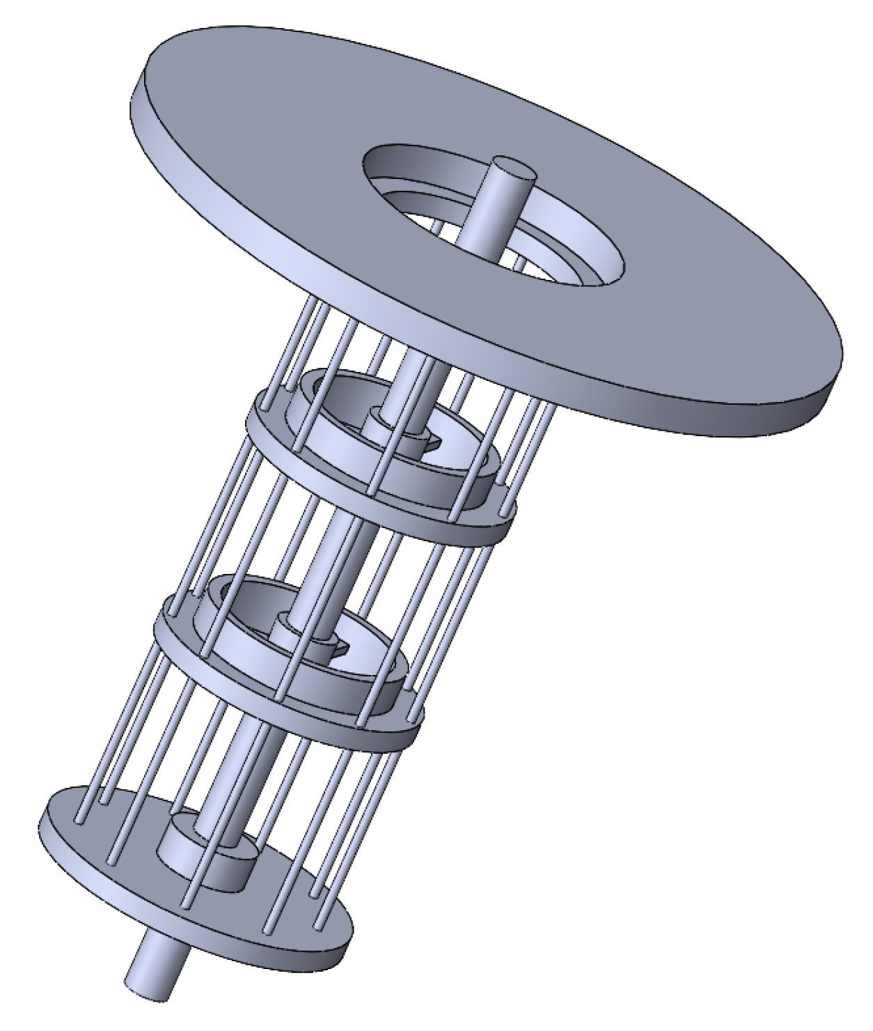
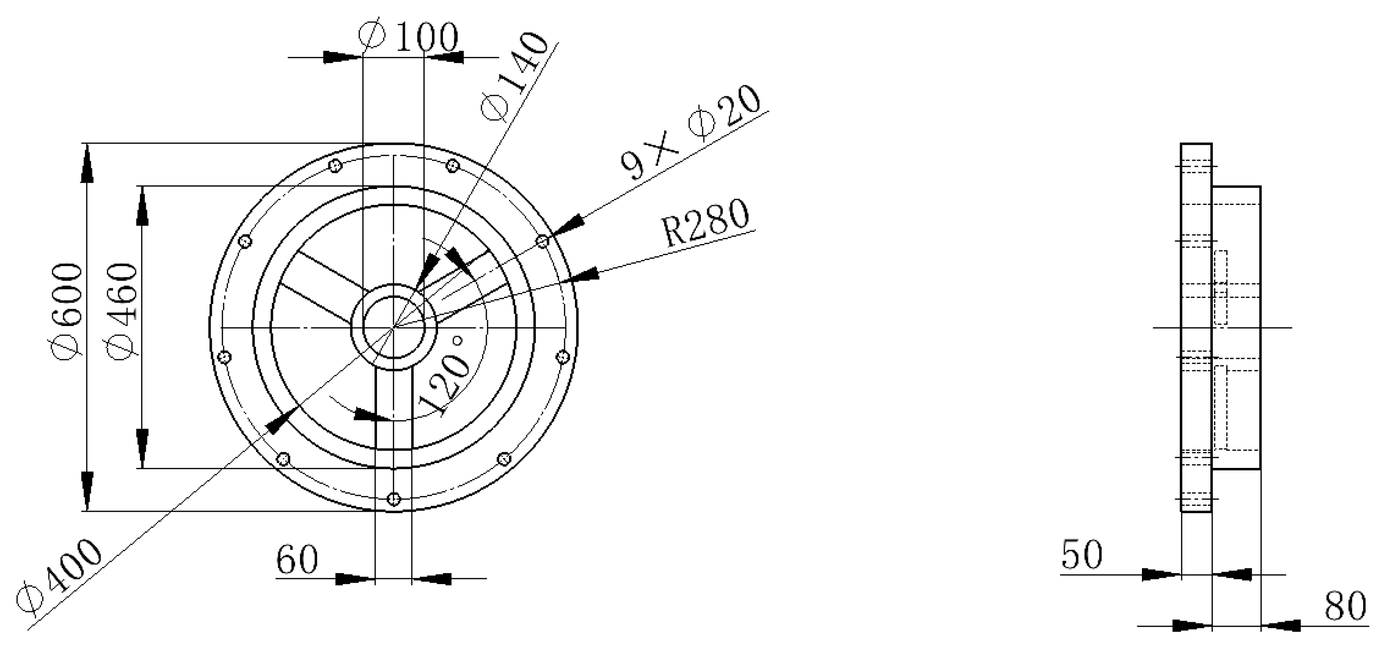
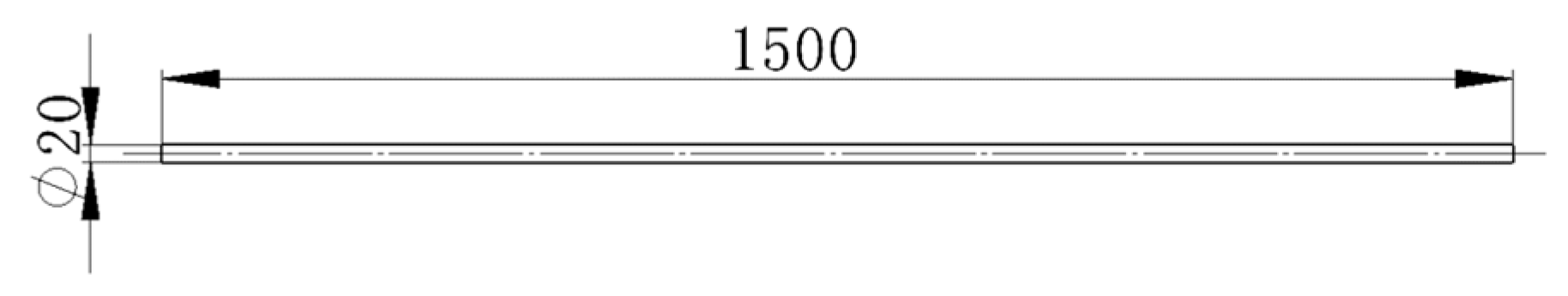
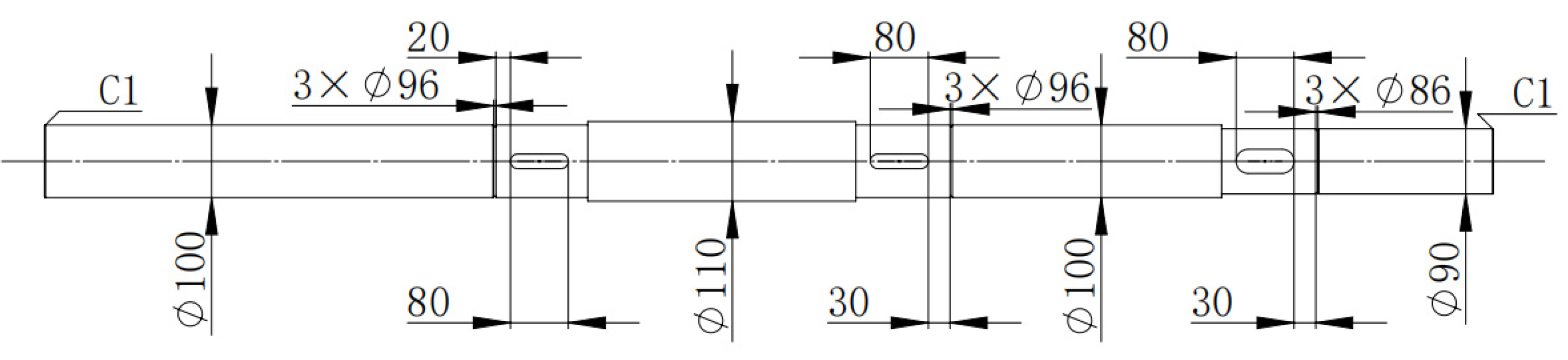
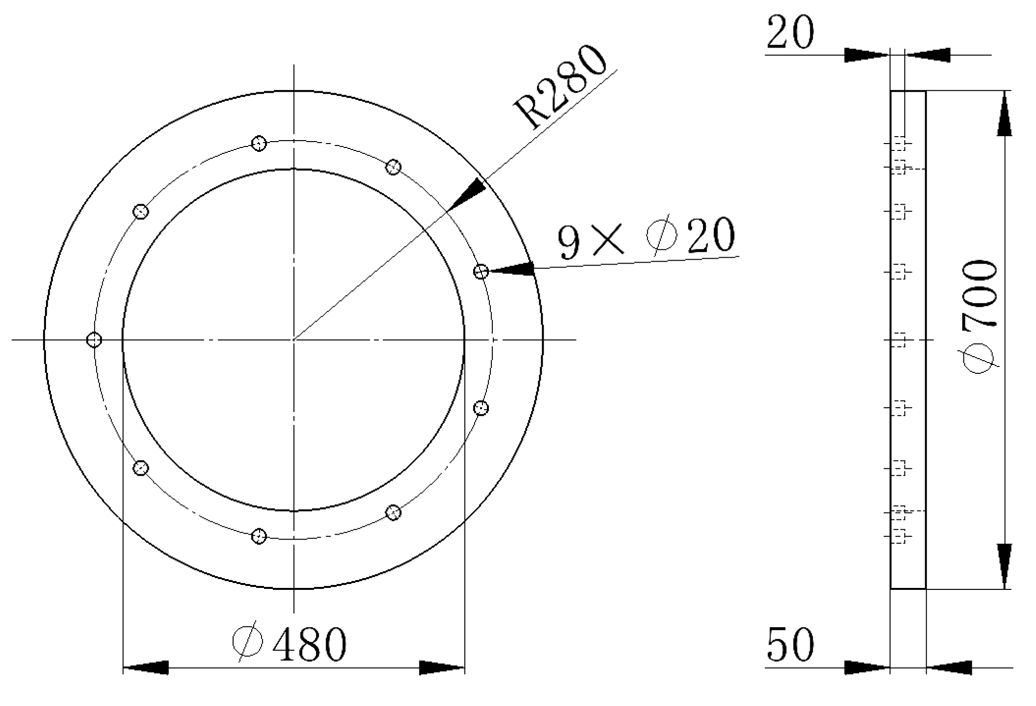
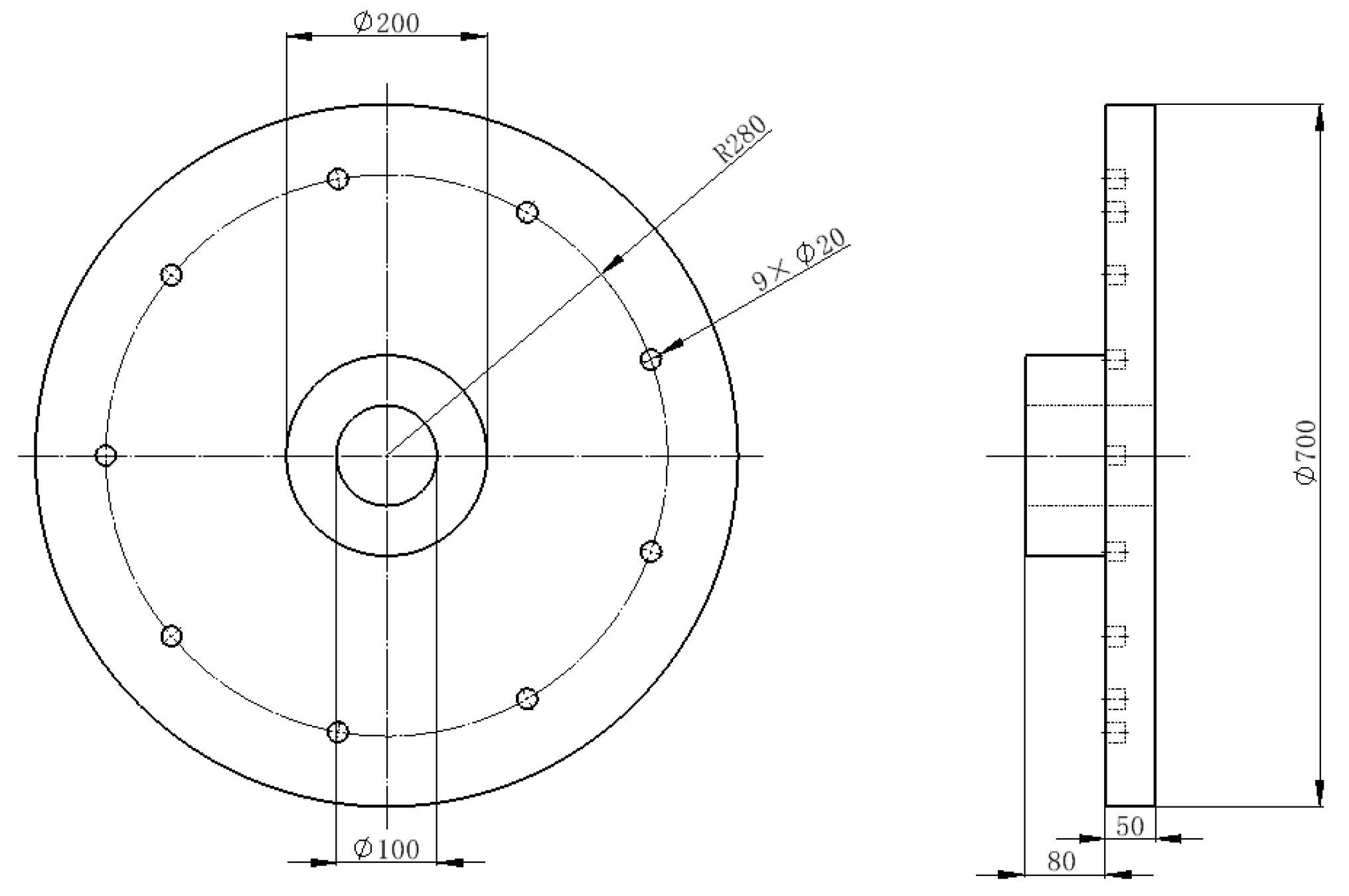
2.1. Spray Tower Model

The spray tower model used in this study is shown in Figure 1.

The impeller dimensions are illustrated in Figure 2.

The impact column dimensions are presented in Figure 3.

The main shaft dimensions are detailed in Figure 4.

The upper base plate dimensions are provided in Figure 5.

The lower base plate dimensions are displayed in Figure 6.

2.2. Governing Equations

The k-ε model was selected for this study due to its established technical advantages in CFD applications, particularly for numerical simulation of high Reynolds number turbulent flows. The standard k-ε model is primarily based on the turbulent kinetic energy equation and the turbulent dissipation rate equation, making it applicable to most engineering problem-solving scenarios. The k-ε equations are formulated as [35,36,37]

$${\displaystyle \frac{\mathrm{D}(\rho k)}{\mathrm{D}t}}={\displaystyle \frac{\partial }{\partial x_j}}\left[\left(\mu +{\displaystyle \frac{{\mu }_{\mathrm{t}}}{{\sigma }_i}}\right){\displaystyle \frac{\partial k}{\partial x_j}}\right]+{\tau }_{ij}{\displaystyle \frac{\partial {\overline{u}}_i}{\partial x_j}}-\rho \epsilon$$

(1)

$${\displaystyle \frac{\mathrm{D}(\rho \epsilon )}{\mathrm{D}t}}={\displaystyle \frac{\partial }{\partial x_j}}\left[\left(\mu +{\displaystyle \frac{{\mu }_{\mathrm{t}}}{{\sigma }_z}}\right){\displaystyle \frac{\partial \epsilon }{\partial x_j}}\right]+C_{\mathrm{z}1}{\displaystyle \frac{\epsilon }{k}}{\tau }_{ij}{\displaystyle \frac{\partial {\overline{u}}_i}{\partial x_j}}-C_{\mathrm{r}2}\rho {\displaystyle \frac{{\epsilon }^2}{k}}$$

(2)

where k represents turbulent kinetic energy (m²/s²), ε denotes turbulent dissipation rate (m²/s³), ρ is fluid density (kg/m³), and μ_t stands for turbulent viscosity. These parameters are defined as

$${\mu }_{\mathrm{t}}=\rho C_p{\displaystyle \frac{k^2}{\epsilon }}$$

(3)

where σ_k = 1.0; σ_ε = 1.3; C_μ = 0.09; C_ε1 = 1.44; and C_ε2 = 1.92.

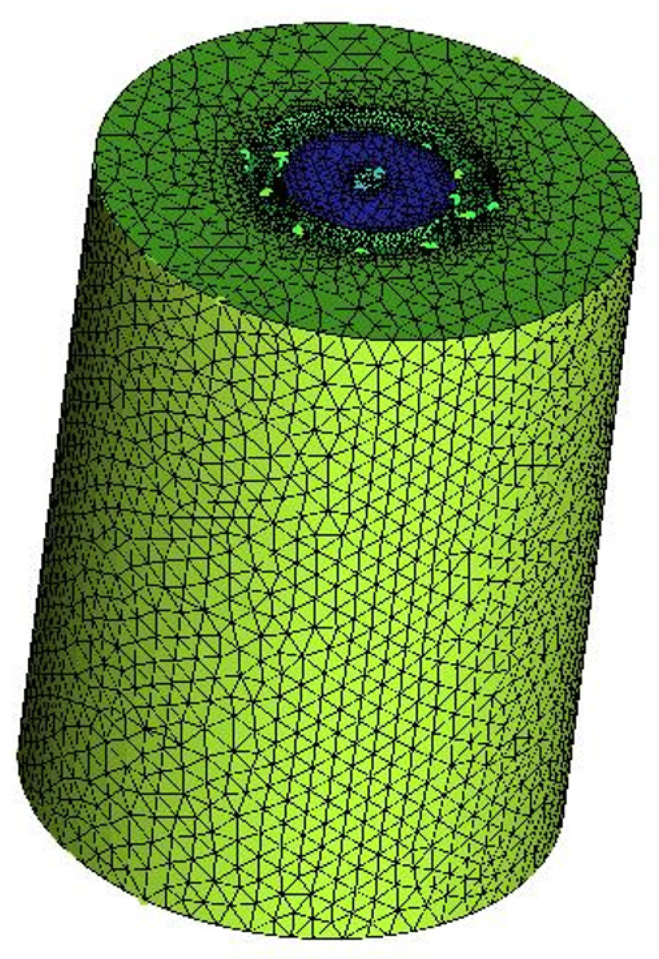
2.3. Mesh Generation

Grid independence verification and grid convergence index (GCI) evaluation [38,39] were conducted on the mesh model. As shown in Figure 7 (the number 1-8 stand for the grid calculation times), when the mesh count exceeded 800,000, the monitored parameters showed no significant changes with further mesh refinement, and the GCI values remained below 5%.

Finally, the final mesh generation diagram for the water domain is shown in Figure 8, consisting of 876,161 mesh elements. The orthogonal quality of the mesh was maintained above 0.2.

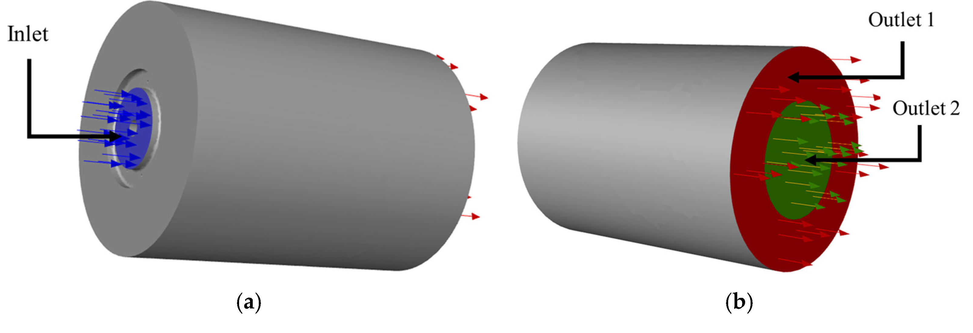
2.4. Boundary Conditions and Computational Methods

The inlet/outlet configuration is illustrated in Figure 9, where outlet 1 serves as the peripheral outlet and outlet 2 functions as the internal outlet. The diameters of these outlets match the installation diameters of the impact columns. The water exiting through outlet 1 can be characterized as an ejected liquid.

A velocity inlet approach was applied to the inlet boundary settings, specifying inlet velocity magnitudes to drive fluid into the system. The outlet boundaries utilized pressure-based free outflow conditions, enabling the fluid to exit naturally in accordance with internal flow dynamics without introducing external constraints.

To systematically investigate parameter effects on system performance, multiple simulations were conducted across varying rotational speeds and inlet water velocities. Specifically, 42 distinct test configurations were established, each corresponding to a unique combination of rotational speed and inlet velocity. Detailed test parameters are listed in

Table 1. Research scheme.

Serial Number	Rotational Speed of Spray Tower (r/min)	Inlet Water Velocity (m/s)	Serial Number	Rotational Speed of Spray Tower (r/min)	Inlet Water Velocity (m/s)
01	300	1	22	600	1
02	300	2	23	600	2
03	300	3	24	600	3
04	300	4	25	600	4
05	300	5	26	600	5
06	300	6	27	600	6
07	300	7	28	600	7
08	400	1	29	700	1
09	400	2	30	700	2
10	400	3	31	700	3
11	400	4	32	700	4
12	400	5	33	700	5
13	400	6	34	700	6
14	400	7	35	700	7
15	500	1	36	800	1
16	500	2	37	800	2
17	500	3	38	800	3
18	500	4	39	800	4
19	500	5	40	800	5
20	500	6	41	800	6
21	500	7	42	800	7

, covering extensive operational conditions to comprehensively analyze flow characteristics and system responses under diverse scenarios.

3. Results Analysis

3.1. Operational Condition Effects

Figure 10 displays the relationship between average outlet velocity and inlet water velocity. The average outlet velocity increases significantly with higher rotational speeds. At 300 r/min, when the inlet water velocity rises from 1 m/s to 7 m/s, the average outlet velocity decreases from 2.927 m/s to 2.328 m/s. The reduction is 0.599 m/s.

At 400 r/min and 500 r/min, increasing the inlet water velocity from 1 m/s to 2 m/s elevates the average outlet velocity. At 400 r/min, it increases from 3.729 m/s to 4.011 m/s, a rise of 0.282 m/s. At 500 r/min, it increases from 4.492 m/s to 5.011 m/s, a rise of 0.519 m/s. However, further increasing the inlet water velocity to 7 m/s causes the average outlet velocity to decline. At 400 r/min, it drops from 4.011 m/s to 3.154 m/s, a reduction of 0.857 m/s. At 500 r/min, it drops from 5.011 m/s to 4.213 m/s, a reduction of 0.798 m/s.

For 600 r/min, 700 r/min, and 800 r/min, raising the inlet water velocity from 1 m/s to 3 m/s significantly increases the average outlet velocity. At 600 r/min, it rises from 5.2 m/s to 6.106 m/s, an increase of 0.906 m/s. At 700 r/min, it rises from 6.021 m/s to 7.084 m/s, an increase of 1.063 m/s. At 800 r/min, it rises from 6.705 m/s to 8.014 m/s, an increase of 1.309 m/s. Beyond 3 m/s inlet water velocity, the average outlet velocity stabilizes and then gradually decreases. At 600 r/min, it falls from 6.106 m/s to 5.173 m/s, a reduction of 0.933 m/s. At 700 r/min, it falls from 7.084 m/s to 6.755 m/s, a reduction of 0.329 m/s. At 800 r/min, it falls from 8.014 m/s to 7.621 m/s, a reduction of 0.393 m/s.

At high rotational speeds (600–800 r/min), the average outlet velocity rises sharply under low inlet water velocities (1–3 m/s) but stabilizes and declines at higher flows. This indicates an efficient low-velocity response, but also reveals limitations due to internal resistance or mixing inefficiency. For mid-range speeds (400–500 r/min), initial velocity gains (1–2 m/s) reverse sharply at higher flows (2–7 m/s) with reductions of 0.798–0.857 m/s. This reflects weak flow regulation due to liquid-phase interference or design constraints. At low speed (300 r/min), continuous velocity decline (−0.599 m/s) suggests insufficient kinetic energy for effective liquid separation under high inlet flows.

The variation of the average flow velocity at outlet 1 is shown in Figure 11. The relationship between average outlet 1 flow velocity and inlet water velocity reveals the dynamic characteristics of internal flow in spray towers. When rotational speed is maintained at 300 r/min, increasing inlet velocity from 1 m/s to 7 m/s causes the average outlet velocity to decrease monotonically from 2.94 m/s to 1.741 m/s, indicating that enhanced fluid resistance suppresses outlet velocity under low-speed conditions. At 400 r/min, the outlet velocity increases from 3.715 m/s to 3.966 m/s as the inlet velocity rises from 1 m/s to 2 m/s, followed by a gradual decrease to 2.454 m/s with a further inlet velocity increase to 7 m/s, showing a nonlinear trend of initial increase followed by a decrease. Similar behavior becomes more pronounced at 500 r/min: the outlet velocity rises from 4.48 m/s to 5.015 m/s when the inlet velocity increases from 1 m/s to 2 m/s, then decreases to 3.468 m/s as the inlet velocity reaches 7 m/s.

Notably, at 600 r/min, the outlet velocity increases from 5.151 m/s to 6.007 m/s with the inlet velocity rising from 1 m/s to 3 m/s, followed by a decrease to 5.194 m/s when the inlet velocity increases to 5 m/s, and further drops to 4.52 m/s at 7 m/s. This multi-stage behavior indicates that enhanced centrifugal force promotes liquid dispersion at high speeds, but flow resistance dominates after exceeding critical inlet velocities. At 700 r/min and 800 r/min, significant velocity increases occur during inlet velocity rise from 1 m/s to 3 m/s (700 r/min: 6.029 m/s to 7.066 m/s; 800 r/min: 6.724 m/s to 7.981 m/s), followed by weakened acceleration and final decreases to 6.174 m/s and 7.137 m/s, respectively, as the inlet velocity reaches 7 m/s. This trend reflects saturated turbulent mixing intensity under high-speed rotation, where excessive inlet velocity intensifies energy dissipation and reduces system efficiency.

Physically, higher rotational speeds intensify centrifugal forces, enhancing liquid interface renewal frequency and improving mass transfer efficiency, particularly at low inlet velocities. However, when inlet velocity surpasses system capacity, liquid retention effects and boundary layer thickening counteract velocity increases, leading to non-monotonic outlet velocity variations.

The average flow velocity variation at outlet 2 is shown in Figure 12. At 300 r/min, increasing the inlet water velocity from 1 m/s to 7 m/s causes the average outlet 2 velocity to rise gradually from 2.893 m/s to 3.815 m/s, showing an overall increasing trend. At 400 r/min, outlet 2 velocity increases from 3.765 m/s to 4.925 m/s with similar inlet velocity adjustments, indicating a more pronounced growth rate compared to the 300 r/min condition. However, at 500 r/min, increasing inlet velocity from 4 m/s to 6 m/s raises outlet 2 velocity from 5.458 m/s to 5.984 m/s, followed by a drop to 5.673 m/s and a subsequent increase to 6.099 m/s at 7 m/s, creating local fluctuations. Similar anomalies occur at 700 r/min: outlet 2 velocity decreases from 7.62 m/s to 7.43 m/s during inlet velocity rise from 4 m/s to 6 m/s, then recovers to 8.226 m/s at 7 m/s. In contrast, outlet 2 velocities at 600 r/min and 800 r/min exhibit continuous increases without significant fluctuations as the inlet velocity rises.

Physically, at low speeds (300–400 r/min), liquid flow remains in low-speed mixing states, where increased inlet kinetic energy directly dominates outlet velocity changes. Beyond 500 r/min, intensified turbulence enhances local resistance coefficients. During inlet velocity increases from 4 m/s to 6 m/s, liquid disturbances convert part of the kinetic energy into turbulent energy, causing temporary velocity drops. Notably, at 800 r/min, outlet 2 velocity rises continuously from 6.655 m/s to 8.85 m/s with inlet velocity increasing from 1 m/s to 7 m/s, demonstrating improved separation efficiency under high-speed rotation, where inlet energy converts more effectively to outlet velocity. Additionally, when the inlet velocity exceeds 5 m/s, velocity growth rates across all rotational speeds plateau, likely due to saturated liquid flux and dynamically balanced flow resistance–energy dissipation mechanisms.

The variation in outlet 1 flow rate with inlet water velocity is shown in Figure 13. The results show the following: At 300 r/min, outlet 1 flow rate decreases continuously from 3.716 m³/s to 2.2 m³/s with inlet water velocity increasing from 1 m/s to 7 m/s, indicating a strong negative correlation. This trend likely stems from insufficient turbulence intensity at low speeds, which limits centrifugal efficiency and hinders effective liquid distribution through outlet channels. At 400 r/min, flow rate increases from 4.695 m³/s to 5.012 m³/s as the inlet velocity rises from 1 m/s to 2 m/s, demonstrating improved phase transfer due to mechanical agitation. However, further inlet velocity increases from 2 m/s to 7 m/s cause the flow rate to drop back to 3.102 m³/s, reflecting suppressed distribution caused by enhanced liquid film resistance under high-velocity conditions.

Similar nonlinear behavior appears at 500 r/min: the flow rate rises from 5.663 m³/s to 6.338 m³/s when the inlet velocity increases from 1 m/s to 2 m/s, then declines to 4.383 m³/s at 7 m/s. Notably, at 600 r/min, the flow rate curve exhibits complex multi-peak characteristics: the flow rate increases significantly from 6.51 m³/s to 7.592 m³/s during 1–3 m/s, drops to 7.278 m³/s at 4 m/s, increases again from 6.564 m³/s to 6.602 m³/s during 5–6 m/s, and finally decreases to 5.712 m³/s at 7 m/s. This pattern suggests a dynamic balance between centrifugal force from rotor rotation and liquid inertia, forming stable separation channels within specific velocity ranges.

At higher speeds (700–800 r/min), outlet 1 flow rate follows new trends: increasing the inlet velocity from 1 m/s to 3 m/s raises the flow rate from 7.619 m³/s to 8.93 m³/s (700 r/min) and from 8.499 m³/s to 10.087 m³/s (800 r/min), showing enhanced phase transfer from increased mechanical energy input. Further inlet velocity increases to 7 m/s cause gradual reductions to 7.803 m³/s (700 r/min) and 9.02 m³/s (800 r/min). This behavior may relate to intensified shear forces at high speeds—when velocity exceeds critical thresholds, excessive turbulence disrupts droplet stability, reduces liquid film thickness, and lowers the effective flow area. Comprehensive analysis reveals that equipment demonstrates superior flow control performance at 600–800 r/min rotational speeds, though inlet velocity should be maintained within 3–5 m/s to avoid flow fluctuations caused by liquid film instability.

The variation in outlet 2 flow rate is shown in Figure 14. The results show the following: As rotational speed increases from 300 r/min to 800 r/min, outlet 2 flow rate exhibits systematic growth. At 300 r/min, increasing the inlet water velocity from 1 m/s to 7 m/s raises the flow rate from 1.453 m³/s to 1.917 m³/s, with a peak of 1.797 m³/s occurring at an inlet velocity of 4 m/s. Notably, at 500 r/min, the flow rate decreases from 3.007 m³/s to 2.85 m³/s when the inlet velocity increases from 5 m/s to 6 m/s. Similar anomalies occur at 700 r/min, where the flow rate drops from 3.828 m³/s to 3.733 m³/s during 4–6 m/s inlet velocity increases. For other conditions, outlet flow rates rise continuously with inlet velocity—e.g., at 800 r/min, the flow rate increases from 3.344 m³/s to 4.446 m³/s as the inlet velocity reaches 7 m/s.

This behavior can be explained through fluid dynamics: Enhanced impeller-driven force at higher rotational speeds increases overall flow rates. However, within specific speed ranges, exceeding critical inlet velocities causes nonlinear changes in mixing efficiency. At 500 r/min, increased kinetic energy at 5–6 m/s inlet velocities triggers localized turbulence, intensifying liquid disturbances and droplet entrainment that reduce effective flow area, manifesting as temporary flow rate drops. Similar effects appear at 700 r/min, where centrifugal–inertial coupling causes fluctuating separation efficiency. When the inlet velocity further increases to 7 m/s, system resistance is gradually overcome by pumping capacity, restoring flow rate growth. This nonlinear response highlights the need to integrate fluid dynamic characteristics with geometric constraints in spray tower parameter optimization.

Figure 15 illustrates the relationship between the inlet water velocity and the outlet 2/outlet 1 flow rate ratio across varying rotational speeds. The results show the following: At 300 r/min, the ratio increases from 0.391 to 0.871 as the inlet velocity rises from 1 m/s to 7 m/s, indicating enhanced centrifugal control over liquid distribution under higher flow velocities. At 400 r/min, the ratio exhibits nonlinear growth, rising from 0.403 to 0.798. Notably, only a 0.057 increase occurs between 2 and 3 m/s, contrasting with the 0.079 increase observed in the same velocity range at 300 r/min. Further analysis reveals that at 500 r/min, the ratio increases from 0.401 to 0.699—showing reduced growth compared to 300 r/min—but experiences a 0.005 negative fluctuation between 1 and 2 m/s, highlighting emerging interactions between rotational speed and flow velocity.

Significantly different behavior appears at 800 r/min: the ratio rises only from 0.393 to 0.493 with the inlet velocity increasing from 1 m/s to 7 m/s, representing a 58% reduction in growth compared to 300 r/min. This stagnation likely stems from intense turbulent effects at high speeds, which disrupt directional transport capabilities by frequently restructuring liquid phases. Additionally, at 600 r/min, the ratio increases from 0.411 to 0.600 before dropping to 0.492, potentially caused by secondary flow disturbances that compromise radial separation mechanisms under combined speed–flow interactions. Physically, centrifugal-driven droplet migration dominates at low speeds, strengthening with increased inlet velocity. However, high-speed conditions introduce additional resistance and turbulent energy dissipation that suppress separation efficiency, ultimately weakening flow rate ratio growth trends.

3.2. Correlation Analysis

For each rotational speed and inlet water velocity scenario, correlation coefficients between parameters were calculated, and correlation analysis was performed for all data groups. The calculation formula, range of values, and evaluation criteria for the correlation coefficient R are as follows:

Calculation formula for correlation coefficient R:

$$R={\displaystyle \frac{{\displaystyle {\sum }_{i=1}^n(X_i-\overline{X})(Y_i-\overline{Y})}}{\sqrt{{\displaystyle {\sum }_{i=1}^n{\left(X_i-\overline{X}\right)}^2}}\sqrt{{\displaystyle {\sum }_{i=1}^n{\left(Y_i-\overline{Y}\right)}^2}}}}$$

(4)

where R represents the correlation coefficient and X and Y denote variable datasets.

The correlation coefficient R falls within the interval −1 ≤ R ≤ +1.

As shown in

Table 2. Judgment criteria of correlation coefficient R.

Value of |R|	Correlation Level
|R| = 0	No correlation
0 ≤ |R| ≤ 0.3	Weak correlation
0.3 ≤ |R| ≤ 0.5	Low correlation
0.5 ≤ |R| ≤ 0.8	Moderate correlation
0.8 ≤ |R| ≤ 1	Strong correlation
|R| = 1	Totally relevant

, a positive R value (>0) indicates a direct correlation, while a negative R value (<0) indicates an inverse correlation.

Correlation coefficients among inlet water velocity, rotational speed, outlet average flow velocity, outlet 1 and 2 flow velocities, outlet 1 and 2 flow rates, and outlet 2/outlet 1 flow rate ratios are presented in

Table 3. Correlation coefficient between rotating speed and various performances.

Variable	vout	vout1	vout2	Qout1	Qout2	Qout2/Qout1
Inlet water velocity at 300 r/min	−0.9551	−0.9831	0.9253	−0.9831	0.9253	0.993
Inlet water velocity at 400 r/min	−0.8855	−0.9427	0.9712	−0.9427	0.9712	0.9564
Inlet water velocity at 500 r/min	−0.6395	−0.8676	0.9185	−0.8676	0.9185	0.9703
Inlet water velocity at 600 r/min	−0.2754	−0.6021	0.9064	−0.6021	0.9064	0.9106
Inlet water velocity at 700 r/min	0.4071	−0.1533	0.9203	−0.1533	0.9203	0.932
Inlet water velocity at 800 r/min	0.5229	0.111	0.9427	0.111	0.9427	0.9515

and

Table 4. Correlation coefficients between inlet water velocity and performance parameters.

Variable	vout	vout1	vout2	Qout1	Qout2	Qout2/Qout1
Rotational speed at 1 m/s	0.9998	0.9996	0.9987	0.9996	0.9987	0.0014
Rotational speed at 2 m/s	0.9972	0.9954	0.9998	0.9954	0.9998	−0.765
Rotational speed at 3 m/s	0.9992	0.9991	0.9974	0.9991	0.9974	−0.9626
Rotational speed at 4 m/s	0.9998	0.9999	0.9961	0.9999	0.9961	−0.8703
Rotational speed at 5 m/s	0.9994	0.9993	0.9941	0.9993	0.9941	−0.9667
Rotational speed at 6 m/s	0.999	0.9974	0.9985	0.9974	0.9985	−0.9574
Rotational speed at 7 m/s	0.9959	0.9933	0.9964	0.9933	0.9964	−0.9918

. This study systematically analyzed flow characteristic relationships through correlations between inlet velocity/rotational speed and performance parameters. The p-values corresponding to R values with absolute magnitudes greater than 0.7 are all less than 0.05, indicating statistical significance.

At 300 r/min, the inlet water velocity showed strong negative correlations with the outlet average velocity, outlet 1 velocity, and outlet 1 flow rate (R = −0.9551, −0.9831, −0.9831), while strong positive correlations were observed with outlet 2 velocity, outlet 2 flow rate, and the outlet 2/outlet 1 ratio (R = 0.9253, 0.9253, 0.9930). The 0.9930 correlation between the outlet 2/outlet 1 ratio and the inlet velocity indicates an extremely significant positive relationship. At 400 r/min, the absolute correlation between inlet velocity and outlet average velocity decreased to 0.8855 but remained significant, with outlet 2-related parameters increasing to 0.9712 and 0.9564. By 500 r/min, the inlet velocity–outlet average velocity correlation weakened to moderate (−0.6395), though outlet 2 parameters maintained strong positive correlations (0.9185, 0.9703). At 600 r/min, the inlet velocity showed a weak negative correlation with outlet average velocity (−0.2754), while outlet 2 parameters retained high correlations (0.9064, 0.9106). Notably, at 700 r/min, the inlet velocity exhibited a low positive correlation with outlet average velocity (0.4071) but maintained strong outlet 2 correlations (0.9203, 0.9320). At 800 r/min, the inlet velocity–outlet average velocity correlation strengthened to moderate (0.5229), with outlet 2 parameters reaching 0.9427 and 0.9515.

Under fixed inlet velocities, rotational speed correlations exhibited distinct patterns. At 1 m/s, the rotational speed showed near-perfect correlations with outlet average velocity and outlet 1 parameters (R = 0.9998, 0.9996, 0.9996), but negligible correlation with the outlet 2/outlet 1 ratio (R = 0.0014). At 2 m/s, the rotational speed–outlet 2/outlet 1 ratio correlation turned strongly negative (−0.765), reaching −0.9626 at 3 m/s. For 4–7 m/s inlet velocities, the rotational speed maintained ultra-high correlations with outlet average velocity and outlet 1 parameters (R = 0.9961–0.9999), while the outlet 2/outlet 1 ratio correlations stabilized in a strong negative range (−0.8703 to −0.9918). These quantitative results illustrate the distinct regulatory influences of inlet velocity and rotational speed on outlet flow fields, particularly highlighting stable negative rotational control over outlet 2/outlet 1 flow distribution under high-speed conditions.

3.3. Flow Field Characteristics

Seven representative cross-sections (Cross-sections 1–7) within the spray tower model were selected to analyze velocity field distribution characteristics. Their spatial positions are illustrated in Figure 16.

As shown in Figure 17, the velocity vector field in Cross-section 1 (near the inlet) exhibits a distinct annular distribution. Water velocities around the impeller shaft and blades reach up to 16 m/s, forming a clear high-speed core region. Radial velocity gradients show exponential decay, decreasing from 16 m/s near the impeller shaft to approximately 4 m/s at greater distances. Flow velocities decrease progressively with increasing distance from the impeller shaft and blades. The velocity contours also reveal significantly lower flow velocities in the inner water region compared to the outer water region.

Cross-section 2 retains the fundamental velocity distribution features of Section 1, as both are axial cross-sections. Velocity contours at Cross-section 2 confirm faster flows near the impeller shaft and blades, with velocities diminishing farther from these components. Consistent with Cross-section 1, the inner water region maintains markedly lower velocities than the outer water region.

As shown in Figure 18, the velocity contour at Cross-section 3 reveals significantly higher flow velocities between the impeller shaft and impeller periphery compared to other regions.

Figure 19 presents velocity distributions across Cross-sections 4 to 7. At Cross-section 4, high water velocity zones are primarily concentrated around the impact column, exhibiting a radial decay pattern from the column center. As the observation point moves away from the column axis, fluid motion intensity decreases significantly, which may be attributed to local energy dissipation and flow structure reorganization. Cross-section 5 analysis reveals that high-velocity fluid remains localized near the impact column, with distribution characteristics similar to the previous cross-section. Velocity attenuation occurs progressively in the direction away from the column, indicating distinct kinetic energy gradients caused by viscous effects and vortex structures. Cross-section 6 observations demonstrate that elevated velocities persist around the impact column, showing strong localized dominance. Fluid velocity declines progressively with increasing distance from the column center, reflecting typical momentum transfer characteristics in the flow field. Cross-section 7 further reveals relatively low overall velocity levels, with both central and boundary regions exhibiting gentle flow patterns, while the transitional zone between them shows slightly higher velocity distribution. This cross-section exhibits significantly lower velocity features compared to adjacent sections, which may correlate with its downstream location distant from the rotating components, leading to substantial fluid energy attenuation in this region.

3.4. Prediction Model

(1)

Gray Prediction Model

The gray prediction model constructs predictive models using newly generated data sequences instead of original data. The algorithm processes original data through operations like accumulation or reduction to derive approximate exponential patterns, which are then used with processed data to build the model. Key advantages include low data requirements (minimum of four data points) and minimal demands on data accuracy and reliability. The model employs differential equations to uncover system characteristics, significantly improving prediction accuracy. It is computationally efficient, easy to validate, and capable of precise data group predictions. The specific prediction steps for the gray model are as follows [40]:

Known data columns:

$$N^{(0)}=(N^{(0)}(1),N^{(0)}(2),\cdots \cdots ,N^{(0)}(n))$$

(5)

Its first-order accumulated generating sequence is

$$N^{(1)}=(N^{(0)}(1),N^{(0)}(1)+N^{(0)}(2),\cdots \cdots ,N^{(0)}(1)+\cdots +N^{(0)}(n))$$

(6)

Establish the gray differential equation:

$$N^{(1)}(k)+a{z}^{(1)}(k)=b,k=2,3,\cdots ,n$$

(7)

The corresponding whitening differential equation is

$${\displaystyle \frac{d{x}^{(1)}}{dt}}+a{N}^{(1)}(t)=b$$

(8)

Note:

$$u={[a,b]}^T,Y={[N^{(0)}(2),N^{(0)}(3),\cdots ,N^{(0)}(n)]}^T$$

(9)

And

$$B=\left[\begin{array}{cc}\begin{array}{c}-z^{(1)}(2)\\ -z^{(1)}(3)\\ ⋮\\ -z^{(1)}(n)\end{array}& \begin{array}{c}1\\ 1\\ ⋮\\ 1\end{array}\end{array}\right]$$

(10)

Using the least square method, the following results are obtained:

$$J(u)={(Y-Bu)}^T(Y-Bu)$$

(11)

The estimated value of u reaching the minimum value is

$$\widehat{u}={[\widehat{a},\widehat{b}]}^T={(B^{T}B)}^{-1}{B}^{T}Y$$

(12)

Therefore, by solving the equation, we can obtain

$${\widehat{N}}^{(1)}(k+1)=\left(N^{(0)}(1)-{\displaystyle \frac{\widehat{b}}{\widehat{a}}}\right)e^{-\widehat{a}k}+{\displaystyle \frac{\widehat{b}}{\widehat{a}}},k=0,1,\cdots ,n-1,\cdots$$

(13)

The model construction. First, establish the gray prediction model using data to obtain predicted values, followed by residual and deviation value tests.

Residual calculation formula:

$$\epsilon (k)={\displaystyle \frac{N^{(0)}(k)-{\widehat{N}}^{(0)}(k)}{N^{(0)}(k)}},k=1,2,\cdots ,n$$

(14)

where ε(k) is the residual value.

Deviation value calculation formula:

$$p(k)={\displaystyle \frac{\epsilon (k)}{N^{(0)}(k)}}\times 100\%$$

(15)

where p(k) is the deviation value.

Finally, prediction models were established between inlet water velocity and outlet parameters at different rotational speeds, including average outlet velocity, average outlet velocity at outlet 1, average outlet velocity at outlet 2, flow rate at outlet 1, flow rate at outlet 2, and the ratio of flow rate at outlet 2 to that at outlet 1. First-order differential equations were applied to solve the models and establish specific equations for each gray prediction model.

(2)

The Partial Least Squares Regression Prediction Model

Let rotational speed and inlet water velocity be independent variables x₁ and x₂, and define dependent variables y₁ to y₆ as average outlet velocity (y₁), average outlet velocity at outlet 1 (y₂), average outlet velocity at outlet 2 (y₃), flow rate at outlet 1 (y₄), flow rate at outlet 2 (y₅), and the ratio of outlet 2 flow rate to outlet 1 flow rate (y₆).

All variables were standardized through normalization processing. The n standardized data matrix for the independent and dependent variables is denoted as [41]

$$H=\left[\begin{array}{cc}{a}_{11}& a_{12}\\ \begin{array}{c}⋮\\ a_{n1}\end{array}& \begin{array}{c}⋮\\ a_{n2}\end{array}\end{array}\right],G=\left[\begin{array}{cc}\begin{array}{c}{b}_{11}\\ ⋮\\ b_{n1}\end{array}& \begin{array}{cc}\begin{array}{c}\cdots \\ \ddots \\ \cdots \end{array}& \begin{array}{c}{b}_{12}\\ ⋮\\ b_{n6}\end{array}\end{array}\end{array}\right]$$

(16)

Extract the first pair of components u₁ and v₁ from the independent and dependent variable groups, aiming to maximize their correlation. Denote the linear combination of the first component as

$$u_1={\alpha }_{11}{x}_1+{\alpha }_{12}{x}_2={\rho }^{(1)T}X$$

(17)

$$v_1={\beta }_{11}{y}_1+\cdots +{\beta }_{16}{y}_6={\gamma }^{(1)T}Y$$

(18)

The score vectors of the first component are obtained from the standardized data matrices H (independent variables) and G (dependent variables) as follows:

$${\widehat{u}}_1=H{\rho }^{(1)}=\left[\begin{array}{cc}\begin{array}{c}{a}_{11}\\ ⋮\\ a_{n1}\end{array}& \begin{array}{c}{a}_{12}\\ ⋮\\ a_{n2}\end{array}\end{array}\right]\left[\begin{array}{c}{\alpha }_{11}\\ {\alpha }_{12}\end{array}\right]$$

(19)

$${\widehat{v}}_1=G{\gamma }^{(1)}=\left[\begin{array}{ccc}{b}_{11}& \cdots & b_{16}\\ ⋮& \ddots & ⋮\\ b_{n1}& \cdots & b_{n6}\end{array}\right]\left[\begin{array}{c}{\beta }_{11}\\ ⋮\\ {\beta }_{16}\end{array}\right]$$

(20)

The covariance between the first pair of components u₁ and v₁ can be calculated using the inner product of their corresponding score vectors:

$$\begin{array}{l}\max ({\widehat{u}}_1{\widehat{v}}_1)=(H{\rho }^{(1)}G{\gamma }^{(1)})={\rho }^{(1)T}{H}^{T}G{\gamma }^{(1)}\\ \hspace{1em}\hspace{1em}s.t.\left\{\begin{array}{c}{\rho }^{(1)T}{\rho }^{(1)}={‖{\rho }^{(1)}‖}^2=1\\ {\gamma }^{(1)T}{\gamma }^{(1)}={‖{\gamma }^{(1)}‖}^2=1\end{array}\right.\end{array}$$

(21)

Using the Lagrange multiplier method, the problem is transformed into solving for unit vectors ρ⁽¹⁾ and γ⁽¹⁾, such that θ₁ = ρ^(1)TH^TGγ⁽¹⁾ is maximized.

$$\gamma (1)={\displaystyle \frac{1}{{\theta }_1}}{G}^{T}H{\rho }^{(1)}$$

(22)

Establish regressions of the dependent variables on u₁ and the independent variables on u₁:

$$\left\{\begin{array}{c}H={\widehat{u}}_1{\sigma }^{(1)T}+H_1\\ G={\widehat{u}}_1{\tau }^{(1)T}+G_1\end{array}\right.$$

(23)

where H₁ and G₁ are the residual matrices between the predicted and original data.

The least squares estimate of the regression coefficient vector is then given by

$$\left\{\begin{array}{c}{\sigma }^{(1)}={\displaystyle \frac{H^T\widehat{u}1}{{‖{\widehat{u}}_1‖}^2}}\\ {\tau }^{(1)}={\displaystyle \frac{G^T{\widehat{u}}_1}{{‖{\widehat{u}}_1‖}^2}}\end{array}\right.$$

(24)

where σ⁽¹⁾ and τ⁽¹⁾ represent the model effect loadings.

Next, the residuals H₁ and G₁ are used to replace H and G, and the above steps are repeated iteratively until the convergence criteria are met.

Finally, the regression equation based on partial least squares is obtained as

$$y_i=c_1{x}_1+c_2{x}_2+c$$

(25)

where c is a constant.

Following model construction, prediction models between rotational speeds, inlet water velocities, and outlet parameters (including average outlet velocity, average outlet velocity at outlet 1, average outlet velocity at outlet 2, flow rate at outlet 1, flow rate at outlet 2, and the ratio of outlet 2 flow rate to outlet 1 flow rate) are summarized in

Table 5. Comparison of velocity parameter models.

Parameter	Model Type	Mean Relative Error Absolute (MRE)	Mean Absolute Error, m/s (MAE)	Proportion of Relative Error Absolute ≤ 10%	Proportion of Relative Error Absolute ≤ 5%
Average outlet velocity	Gray prediction model	1.879607	0.092669	0.988095	0.928571
Average outlet velocity	Partial least squares regression model	5.109452	0.248564	0.904762	0.47619
Average velocity at outlet 1	Gray prediction model	2.401143	0.108914	0.964286	0.892857
Average velocity at outlet 1	Partial least squares regression model	8.836238	0.3549	0.666667	0.333333
Average velocity at outlet 2	Gray prediction model	2.13869	0.129914	0.97619	0.904762
Average velocity at outlet 2	Partial least squares regression model	8.36869	0.465669	0.738095	0.404762

.

(3)

Prediction Results

To more intuitively compare the performance differences between the gray prediction model and the partial least squares regression model, Table 5 and

Table 6. Comparison of flow rate parameter models.

Parameter	Model Type	Mean Relative Error Absolute (MRE)	Mean Absolute Error, m3/s (MAE)	Proportion of Relative Error Absolute ≤ 10%	Proportion of Relative Error Absolute ≤ 5%
Flow rate at outlet 1	Gray prediction model	2.401143	0.13767	0.964286	0.892857
Flow rate at outlet 1	Partial least squares regression model	8.836238	0.448543	0.666667	0.333333
Flow rate at outlet 2	Gray prediction model	2.13869	0.065267	0.97619	0.904762
Flow rate at outlet 2	Partial least squares regression model	8.36869	0.233945	0.738095	0.404762
Ratio of flow rate at outlet 2 to outlet 1	Gray prediction model	3.34369	0.018844	0.952381	0.880952
Ratio of flow rate at outlet 2 to outlet 1	Partial least squares regression model	15.20321	0.07819	0.380952	0.238095

present the prediction metrics for velocity parameters and flow rate parameters, respectively. These tables clearly illustrate the performance differences between the two models across various parameters.

The gray prediction model exhibits significant performance advantages in predicting velocity and flow rate parameters. As shown in Table 5 (velocity parameter comparison), the mean relative error (MRE) of the gray model ranges from 1.88% to 2.40%, with the lowest MRE for average outlet velocity (1.88%) and the highest for average velocity at outlet 1 (2.40%). The mean absolute error (MAE) is concentrated between 0.09 and 0.13 m/s, far below the 0.25–0.47 m/s range of the partial least squares regression model. Deviation distribution analysis reveals that the proportion of absolute relative deviations ≤10% exceeds 96.4% for all parameters, with achievement rates reaching 98.8% for average outlet velocity and 97.6% for outlet 2 average velocity. In contrast, the partial least squares model drops to 66.7% for outlet 1 average velocity. For deviations ≤5%, the gray model achieves 89.3–92.9% accuracy, with 92.9% for average outlet velocity, while the partial least squares model only attains 33.3–40.5% for outlets 1 and 2. Notably, the gray model’s prediction accuracy for outlet 1 average velocity (MRE = 2.40%) remains superior to the partial least squares model (8.84%), with error fluctuations reduced to 32.7% of the latter’s magnitude.

Table 6 (flow rate parameter comparison) further validates the gray model’s stability. Its MRE ranges from 2.14% (outlet 2 flow rate) to 3.34% (flow rate ratio). The MAE values cluster within 0.065–0.138 m³/s, significantly outperforming the partial least squares model (0.234–0.449 m³/s). For deviations ≤10%, the gray model maintains 95.2–97.6% achievement rates, whereas the partial least squares model drops to 38.1% for the flow rate ratio. Deviations ≤5% achieve 88.1–90.5% in the gray model, compared to 23.8% for the partial least squares model on the flow rate ratio. Critically, the flow rate ratio prediction error surges from 3.34% (gray) to 15.20% (partial least squares), with a 61.1 percentage-point gap in achievement rates.

The gray prediction model effectively suppresses stochastic disturbances in hydrodynamic parameters through its accumulated generating sequence. Its exponential fitting capability enables exceptional performance in trend-driven parameters like average outlet velocity (MRE = 1.88%). In contrast, the partial least squares model loses critical dynamic features during principal component extraction, causing severe accuracy degradation for nonlinearly coupled parameters such as the flow rate ratio (MRE = 15.20%). Computationally, the gray model requires only 12–18% of the partial least squares’ runtime, making it suitable for real-time operational forecasting. Under extreme conditions (e.g., 700 r/min rotational speed or 6 m³/s inlet velocity), the gray model maintains error fluctuations within ±0.5%, while the partial least squares model exhibits up to 12.4% deviation in outlet 1 flow rate predictions. This disparity arises from the gray model’s weakening of raw data volatility via AGO operations, whereas the partial least squares struggles to establish stable principal component spaces under low sample counts (n < 30).

The gray prediction model demonstrates outstanding robustness in velocity parameter prediction, reducing error fluctuations by 62.3–89.5% compared to the partial least squares model, with achievement rates improved by 15.2–28.4 percentage points. It is particularly suited for engineering applications requiring high prediction accuracy and real-time responsiveness. For nonlinearly correlated parameters like flow rate ratios, hybrid models combining gray prediction with support vector regression are recommended to further enhance precision. The partial least squares model remains viable for large datasets (n > 50) but requires strict principal component control via cross-validation to mitigate overfitting risks.

4. Conclusions

This study systematically investigated the relationship between flow characteristics and operational parameters (inlet water velocity and rotational speed) of spray towers through numerical simulation and data analysis methods. The research results demonstrate significant correlations between tower performance and operational parameters, with the following conclusions:

(1)

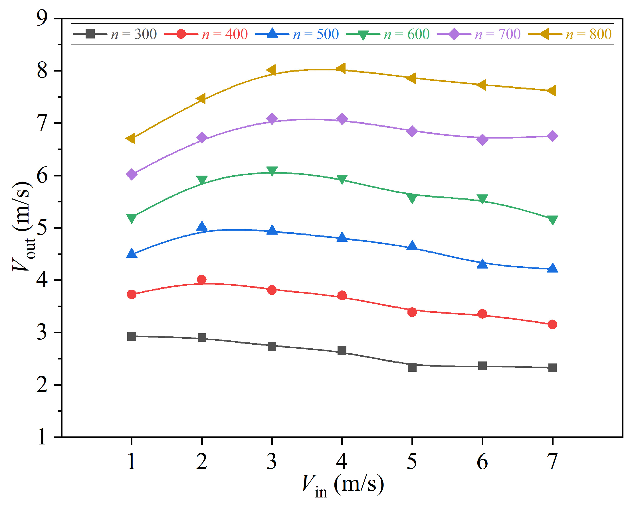
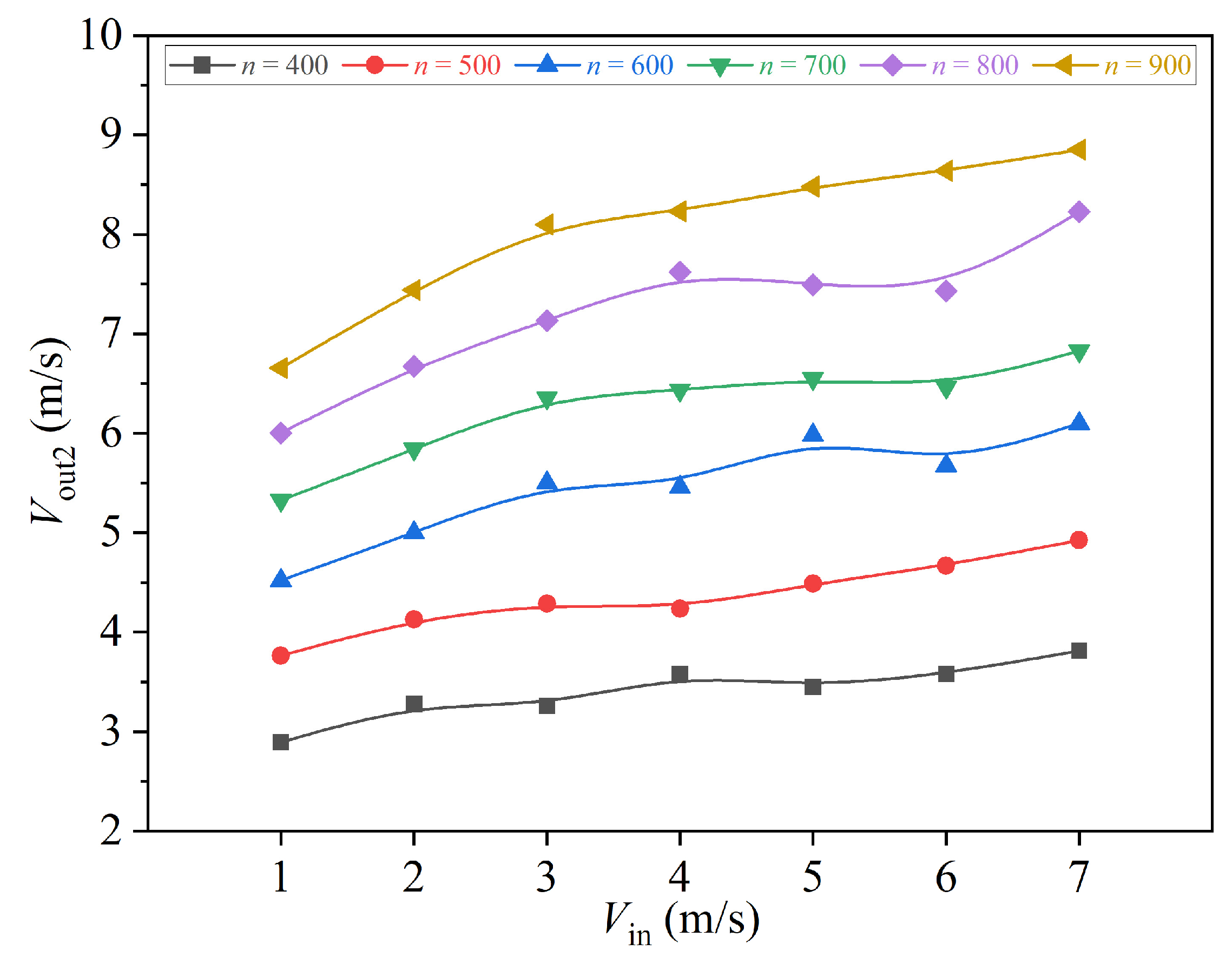
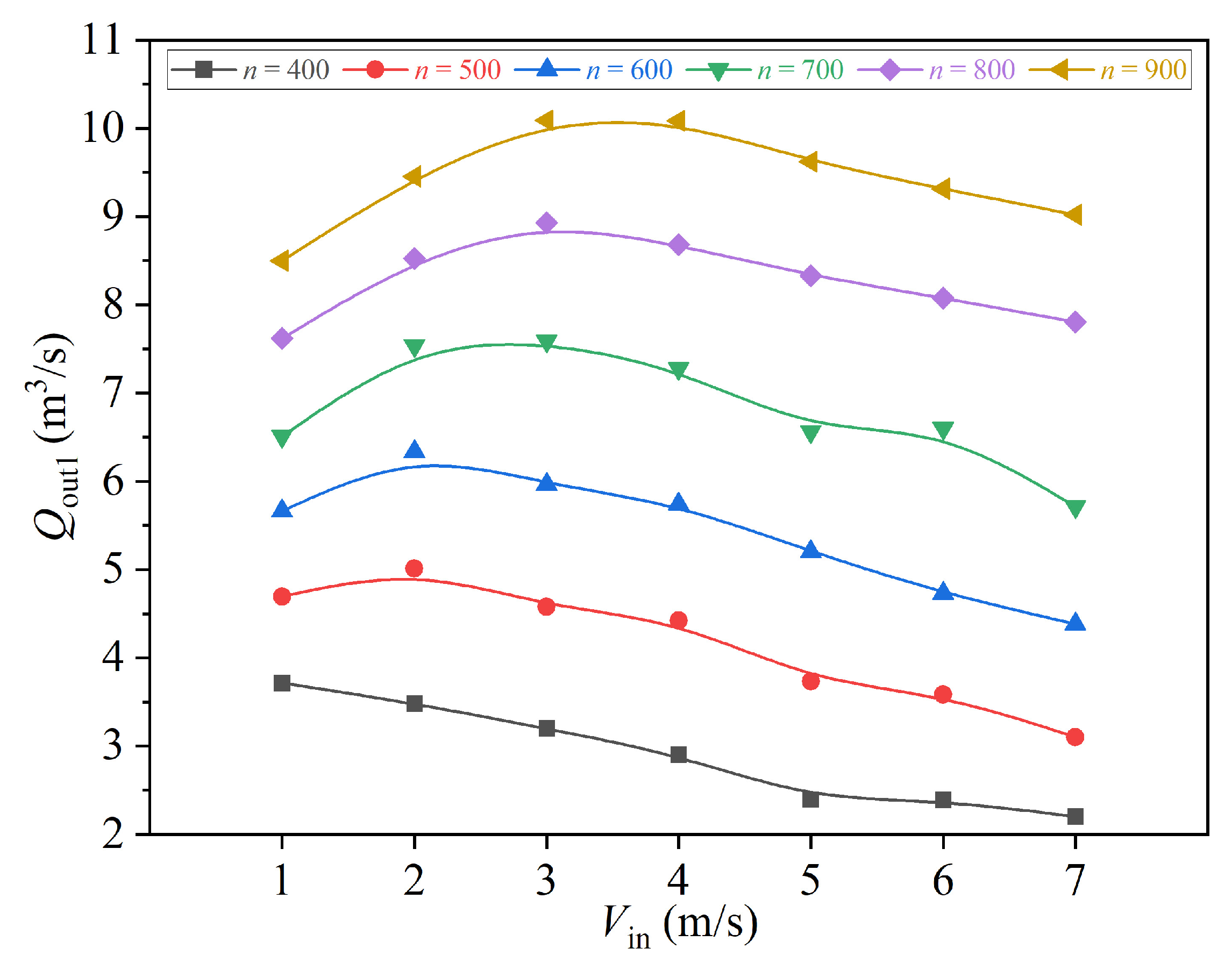
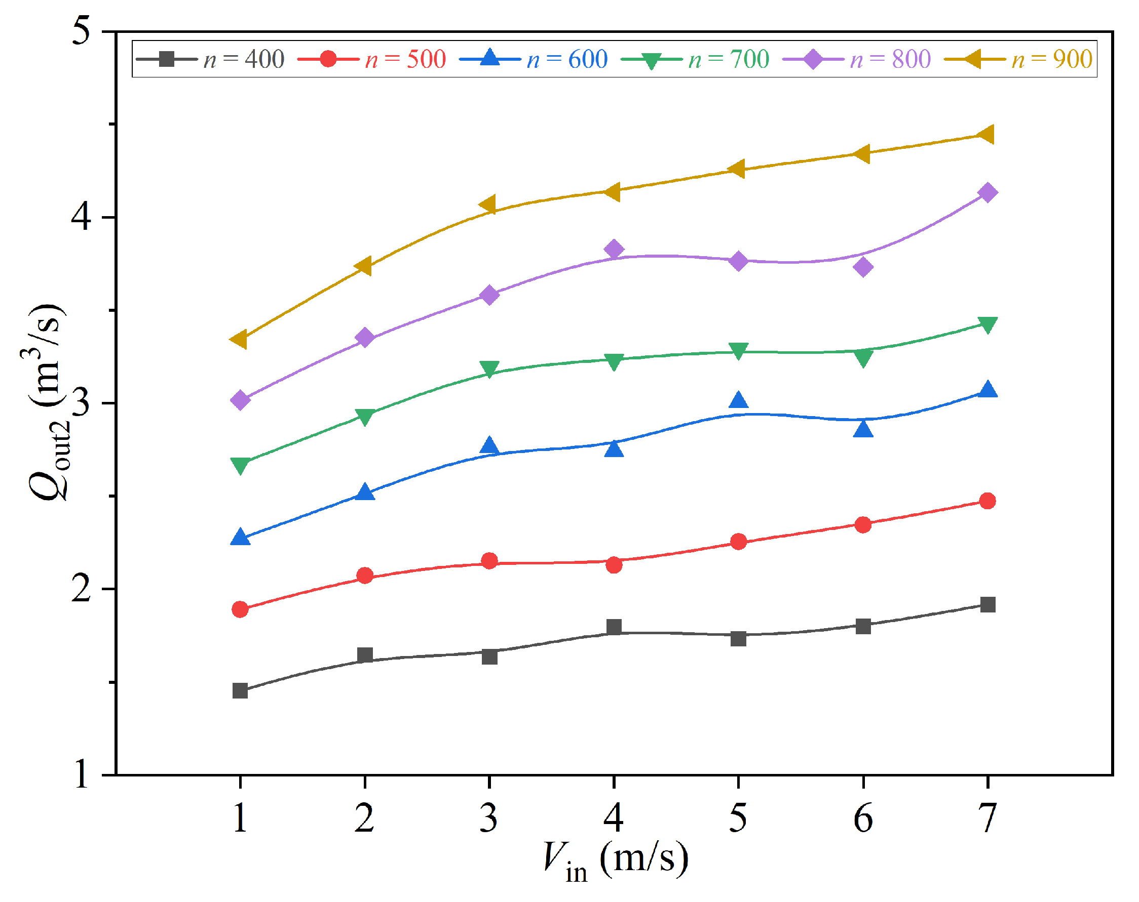
Increased rotational speed (300–800 r/min) significantly enhances outlet flow rate (outlet 2 increases from 1.453 m³/s to 4.446 m³/s) and velocity, particularly in higher rotational speed ranges (600–800 r/min). Inlet water velocity exhibits nonlinear effects: it suppresses flow velocity at low speeds while initially promoting but later reducing flow due to resistance at medium-high speeds. Synergistic control of rotational speed and water volume is required to optimize separation efficiency.

(2)

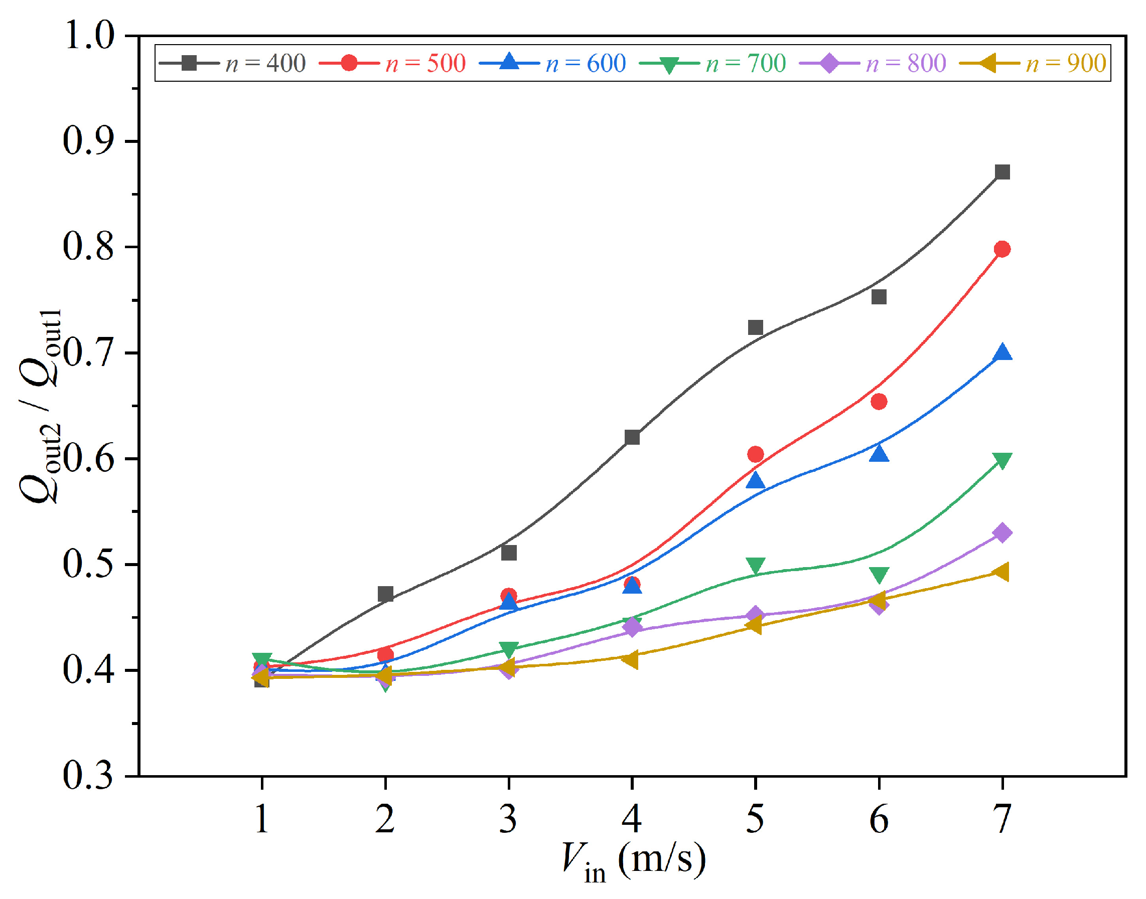
The correlation between inlet water velocity and outlet velocity varies with rotational speed (negative correlation at low speeds, R = −0.9831; weak positive correlation at high speeds, R = 0.5229). The ratio of outlet 2 to outlet 1 flow rate shows a strong negative correlation with rotational speed (R = −0.9918). When rotational speed exceeds 500 r/min, turbulent disturbances weaken centrifugal effects, stabilizing flow distribution and highlighting rotational speed’s dominant role in liquid phase allocation.

(3)

The gray model demonstrates high accuracy (minimum MRE of 1.88%), stability, and efficiency in flow velocity and rate predictions, outperforming the partial least squares model. It is particularly suitable for high real-time requirement scenarios. Future work will integrate more precise computational methods or machine learning algorithms to enhance transient flow velocity capture and improve parameter optimization design.

References

1. Danzomo, B.A.; Umar, S.A.; Salami, M.J.E. Wet Scrubber Design. In Control Engineering in Robotics and Industrial Automation: Malaysian Society for Automatic Control Engineers (MACE) Technical Series 2018; Springer International Publishing: Cham, Switzerland, 2021; pp. 19–62. [Google Scholar] [CrossRef]
2. Bozorgi, Y.; Keshavarz, P.; Taheri, M.; Fathikaljahi, J. Simulation of a spray scrubber performance with Eulerian/Lagrangian approach in the aerosol removing process. J. Hazard. Mater. 2006, 137, 509–517. [Google Scholar] [CrossRef] [PubMed]
3. Mohan, B.R.; Jain, R.; Meikap, B. Comprehensive analysis for prediction of dust removal efficiency using twin-fluid atomization in a spray scrubber. Sep. Purif. Technol. 2008, 63, 269–277. [Google Scholar] [CrossRef]
4. Yao, J.; Tanaka, K.; Kawahara, A.; Sadatomi, M. Geometrical Effects on Spray Performance of a Special Twin-fluid Atomizer without Water Power and its CO2 Absorption Capacity. Jpn. J. Multiph. FLOW 2014, 27, 511–520. [Google Scholar] [CrossRef]
5. Zhang, Q.; Wang, S.; Zhu, P.; Wang, Z.; Zhang, G. Full-scale simulation of flow field in ammonia-based wet flue gas desulfurization double tower. J. Energy Inst. 2018, 91, 619–629. [Google Scholar] [CrossRef]
6. Zeng, F.; Yin, L.; Chen, L. Numerical simulation and optimized design of the wet flue gas desulphurization spray tower. In Challenges of Power Engineering and Environment: Proceedings of the International Conference on Power Engineering 2007; Springer: Berlin/Heidelberg, Germany, 2007; pp. 783–787. [Google Scholar] [CrossRef]
7. Kallinikos, L.; Farsari, E.; Spartinos, D.; Papayannakos, N. Simulation of the operation of an industrial wet flue gas desulfurization system. Fuel Process. Technol. 2010, 91, 1794–1802. [Google Scholar] [CrossRef]
8. Leng, Y.; Hu, R.; Cui, L.; Dong, Y. Study on energy efficiency characteristics of wet flue gas desulfurization tower. Power Gener. Technol. 2020, 41, 543. [Google Scholar] [CrossRef]
9. Schwarz, A.D.; König, L.; Meyer, J.; Dittler, A. Impact of water droplet and humidity interaction with soluble particles on the operational performance of surface filters in gas cleaning applications. J. Aerosol Sci. 2020, 142, 105523. [Google Scholar] [CrossRef]
10. Wang, S.; Zhu, P.; Zhang, G.; Zhang, Q.; Wang, Z.; Zhao, L. Numerical simulation research of flow field in ammonia-based wet flue gas desulfurization tower. J. Energy Inst. 2015, 88, 284–291. [Google Scholar] [CrossRef]
11. Kaltenbach, C.; Laurien, E. CFD simulation of spray cooling in the model containment THAI. Nucl. Eng. Des. 2018, 328, 359–371. [Google Scholar] [CrossRef]
12. Wang, B.; Huang, Y.; Yuan, Y.C. Modeling Spray Formed by Spring Nozzle Using Volume-of-Fluid Method. Adv. Mater. Res. 2011, 354–355, 499–503. [Google Scholar] [CrossRef]
13. Zhang, Z.; Lei, F.; Ma, L.; Du, J.; Zhao, H.; Zhao, Y.; Yuan, J. Research on parameter optimisation of closed wet cooling tower for oil and gas fields. Int. J. Ambient. Energy 2025, 46, 2508344. [Google Scholar] [CrossRef]
14. Xu, M.; Cao, L.; Luo, H.; Hu, P.; Wang, Y. Effect of water spray in exhaust passage of steam turbine on flow field of the last stage during windage. Int. J. Heat Mass. Transf. 2020, 161, 120296. [Google Scholar] [CrossRef]
15. Javed, K.; Mahmud, T.; Purba, E. Enhancement of Mass Transfer in a Spray Tower Using Swirling Gas Flow. Chem. Eng. Res. Des. 2006, 84, 465–477. [Google Scholar] [CrossRef]
16. Jafari, M.J.; Matin, A.H.; Rahmati, A.; Azari, M.R.; Omidi, L.; Hosseini, S.S.; Panahi, D. Experimental optimization of a spray tower for ammonia removal. Atmos. Pollut. Res. 2018, 9, 783–790. [Google Scholar] [CrossRef]
17. Licht, W.; Conway, J.B. Mechanism of Solute Transfer in Spray Towers. Ind. Eng. Chem. 1950, 42, 1151–1157. [Google Scholar] [CrossRef]
18. Darake, S.; Hatamipour, M.; Rahimi, A.; Hamzeloui, P. SO2 removal by seawater in a spray tower: Experimental study and mathematical modeling. Chem. Eng. Res. Des. 2016, 109, 180–189. [Google Scholar] [CrossRef]
19. Dimiccoli, A.; Di Serio, M.; Santacesaria, E. Mass Transfer and Kinetics in Spray-Tower-Loop Absorbers and Reactors. Ind. Eng. Chem. Res. 2000, 39, 4082–4093. [Google Scholar] [CrossRef]
20. Ochowiak, M.; Włodarczak, S.; Pavlenko, I.; Janecki, D.; Krupińska, A.; Markowska, M. Study on Interfacial Surface in Modified Spray Tower. Processes 2019, 7, 532. [Google Scholar] [CrossRef]
21. Ma, S.; Zang, B.; Song, H.; Chen, G.; Yang, J. Research on mass transfer of CO2 absorption using ammonia solution in spray tower. Int. J. Heat Mass. Transf. 2013, 67, 696–703. [Google Scholar] [CrossRef]
22. Chen, Z.; Wang, H.; Zhuo, J.; You, C. Experimental and numerical study on effects of deflectors on flow field distribution and desulfurization efficiency in spray towers. Fuel Process. Technol. 2017, 162, 1–12. [Google Scholar] [CrossRef]
23. Bandyopadhyay, A.; Biswas, M.N. Modeling of SO2 scrubbing in spray towers. Sci. Total. Environ. 2007, 383, 25–40. [Google Scholar] [CrossRef] [PubMed]
24. Cui, H.; Li, N.; Wang, X.; Peng, J.; Li, Y.; Wu, Z. Optimization of reversibly used cooling tower with downward spraying. Energy 2017, 127, 30–43. [Google Scholar] [CrossRef]
25. Wu, X.; Sharif, M.; Yu, Y.; Chen, L.; Zhang, Z.; Wang, G. Hydrodynamic mechanism study of the diameter-varying spray tower with atomization impinging spray. Sep. Purif. Technol. 2021, 268, 118608. [Google Scholar] [CrossRef]
26. Hou, B.; Chen, O.; Wang, Y.; Wang, F.; Lu, G. Structural optimization and flow field simulation of gas distribution device in desulfurization tower. Asia-Pacific J. Chem. Eng. 2023, 19, e2988. [Google Scholar] [CrossRef]
27. Zhong, Y.; Gao, X.; Huo, W.; Luo, Z.-Y.; Ni, M.-J.; Cen, K.-F. A model for performance optimization of wet flue gas desulfurization systems of power plants. Fuel Process. Technol. 2008, 89, 1025–1032. [Google Scholar] [CrossRef]
28. Hong, M.; Xu, G.; Lu, P.; Huang, Z.; Miao, H.; Zhang, Y.; Ma, C.; Zhang, Q. CFD analysis of the spray droplet parameters effect on gas-droplet flow and evaporation characteristics in circulating fluidized bed desulfurization tower. Chem. Eng. Res. Des. 2023, 196, 184–203. [Google Scholar] [CrossRef]
29. Chen, S.; Zhao, X.; Xiao, Z.; Cheng, M.; Zou, R.; Luo, G. Enhancement of fine particle removal through flue gas cooling in a spray tower with packing materials. J. Hazard. Mater. 2024, 478, 135390. [Google Scholar] [CrossRef] [PubMed]
30. Salins, S.S.; Kumar, S.; Chouhan, J.; Tejero-González, A.; Nair, P.S. Experimental performance of a spray tower system for water desalination and indoor thermal comfort. Process. Saf. Environ. Prot. 2023, 180, 122–135. [Google Scholar] [CrossRef]
31. Huang, J.; Zeng, Z.; Hong, F.; Yang, Q.; Wu, F.; Peng, S. Sustainable Operation Strategy for Wet Flue Gas Desulfurization at a Coal-Fired Power Plant via an Improved Many-Objective Optimization. Sustainability 2024, 16, 8521. [Google Scholar] [CrossRef]
32. Zhevzhyk, O.; Potapchuk, I.; Pertsevyi, V.; Bosyi, D.; Biriukov, D.; Shevchenko, S. Numerical modeling of the thermal characteristics of a fan spray cooling tower. Proc. IOP Conf. Ser. Earth Environ. Sci. 2024, 1348, 012090. [Google Scholar] [CrossRef]
33. Valera, V.Y.; Martins, T.D.; Codolo, M.C. Experimental evaluation and neural networks modeling of removal efficiency and volumetric mass transfer coefficient for gas desulfurization in spray tower. Chem. Eng. Sci. 2023, 285, 119568. [Google Scholar] [CrossRef]
34. Ghosh, D.; Biswas, D.; Datta, A. Absorption height in spray tower for wet-limestone process in flue gas desulphurization. Mater. Today Proc. 2024. [Google Scholar] [CrossRef]
35. Zhu, S.; Zhu, Q. Numerical study on the heat transfer performance of a novel spray tower. J. Phys. Conf. Ser. 2020, 1600, 012023. [Google Scholar] [CrossRef]
36. Zhang, T.; Tang, Q.; Pu, C.; Zhang, L. Numerical simulation of gas-droplets mixing and spray evaporation in rotary spray desulfurization tower. Adv. Powder Technol. 2022, 33, 103420. [Google Scholar] [CrossRef]
37. Reuter, H.C.R.; Viljoen, D.J.; Kröger, D.G. A method to determine the performance characteristics of cooling tower spray zones. In Proceedings of the 2010 14th International Heat Transfer Conference, Washington, DC, USA, 8–13 August 2010; Volume 49392, pp. 619–628. [Google Scholar] [CrossRef]
38. Ye, J.-G.; Xu, S.-S.; Huang, H.-F.; Zhao, Y.-J.; Zhou, W.; Zhang, Y.-L. Optimization Design of Nozzle Structure Inside Boiler Based on Orthogonal Design. Processes 2023, 11, 2923. [Google Scholar] [CrossRef]
39. Baker, N.; Kelly, G.; O’SUllivan, P.D. A grid convergence index study of mesh style effect on the accuracy of the numerical results for an indoor airflow profile. Int. J. Vent. 2019, 19, 300–314. [Google Scholar] [CrossRef]
40. Ma, X.; Wu, W.; Zhang, Y. Application of a novel quadratic polynomial discrete grey model to forecast energy consumption of China. Sci. Iran. 2024, 31, 469–480. [Google Scholar] [CrossRef]
41. Wang, J.; Zhang, H.; Hou, P.; Jia, X. A novel prediction model of desulfurization efficiency based on improved FCM-PLS-LSSVM. Multimed. Tools Appl. 2022, 82, 5685–5708. [Google Scholar] [CrossRef]
Figure 1. Spray tower model.
Processes 13 02308 g001
Figure 2. Impeller dimensions.
Processes 13 02308 g002
Figure 3. Impact column dimensions.
Processes 13 02308 g003
Figure 4. Main shaft dimensions.
Processes 13 02308 g004
Figure 5. Upper base plate dimensions.
Processes 13 02308 g005
Figure 6. Lower base plate dimensions.
Processes 13 02308 g006
Figure 7. Grid independence verification: (a) detection value; (b) GCI value.
Processes 13 02308 g007
Figure 8. Mesh generation model.
Processes 13 02308 g008
Figure 9. Inlet and outlet boundary conditions: (a) inlet; (b) outlet.
Processes 13 02308 g009
Figure 10. Effect of inlet water velocity on average outlet velocity.
Processes 13 02308 g010
Figure 11. Variation in average velocity at outlet 1.
Processes 13 02308 g011
Figure 12. Variation in average velocity at outlet 2.
Processes 13 02308 g012
Figure 13. Flow change at outlet 1.
Processes 13 02308 g013
Figure 14. Flow change at outlet 2.
Processes 13 02308 g014
Figure 15. Variation in flow ratio at outlet 2 and outlet 1.
Processes 13 02308 g015
Figure 16. Position of each cross-section.
Processes 13 02308 g016
Figure 17. Velocity contour: (a) Cross-section 1; (b) Cross-section 2.
Processes 13 02308 g017
Figure 18. Velocity contour at Cross-section 3.
Processes 13 02308 g018
Figure 19. Velocity contour: (a) Cross-section 4; (b) Cross-section 5; (c) Cross-section 6; (d) Cross-section 7.
Processes 13 02308 g019aProcesses 13 02308 g019b