Modeling Renewable Energy Feed-In Dynamics in a German Metropolitan Region

Abstract

This study presents community-specific modeling approaches for simulating power injection from photovoltaic and wind energy systems in a German metropolitan region. Developed within the EMN_SIM project and based on openly accessible datasets, the methods are broadly transferable across Germany. For PV, a cluster-based model groups systems by geographic and technical characteristics, using real weather data to reduce computational effort. Validation against measured specific yields shows strong agreement, confirming energetic accuracy. The wind model operates on a per-turbine basis, integrating technical specifications, land use, and high-resolution wind data. Energetic validation indicates good consistency with Bavarian reference values, while power-based comparisons with selected turbines show reasonable correlation, subject to expected limitations in wind data resolution. The resulting high-resolution generation profiles reveal spatial and temporal patterns valuable for grid planning and targeted policy design. While further validation with additional measurement data could enhance model precision, the current results already offer a robust foundation for urban energy system analyses and future grid integration studies.

1. Introduction

Germany’s pursuit of carbon neutrality has accelerated the decentralization of energy production, driven largely by the rapid integration of renewable energy sources (RESs) such as photovoltaics (PV) and wind power. While this transformation supports national climate objectives, it significantly alters the spatio-temporal dynamics of electricity feed-in, shifting the operational burden from traditionally centralized transmission systems to increasingly decentralized distribution grids. The fluctuating and spatially dispersed nature of RES introduces new challenges for grid operation, including voltage regulation, load balancing, and real-time control. As Iweh et al. [1] emphasize, the rise of distributed generation entails technical and operational shifts such as bi-directional power flows, local congestion, and the need for smarter grid interfaces. In addition, Oyekale et al. [2] highlight how the high penetration of inverter-based RES reduces system inertia and can exacerbate frequency and voltage instability, reinforcing the urgency for advanced control strategies and infrastructure reinforcement. Understanding these impacts is critical for resilient infrastructure planning in a decarbonized energy system.

Numerous studies have explored the effects of RES integration on power grid infrastructure and developed various modeling approaches to assess load flows, grid stress, and system stability under high-RES-penetration scenarios [3,4,5]. For example, Saha et al. [6] analyzed the frequency dynamics of low-inertia grids under high renewable shares using dynamic eigenvalue-based stability models. While such studies offer valuable insights at the system level, traditional power flow studies generalize spatial distribution patterns or lack the granularity needed to capture localized dynamics—particularly in multi-sectoral interregional contexts where urban energy demands interact with rural renewable feed-in.

This lack of spatial resolution limits the ability of planners and policymakers to make informed, location-specific decisions that account for both technical constraints and strategic objectives. To address this gap, modeling approaches must evolve to reflect the spatial heterogeneity of RES deployment and local grid infrastructure, enabling accurate assessments of distribution-level stress, congestion, and flexibility requirements. Such fine-grained analyses are essential to design cost-effective interventions—such as localized storage, grid-forming inverter deployment, or targeted reinforcement—that enhance system reliability and facilitate the continued expansion of decentralized renewables.

To address this modeling gap, the Klimapakt2030plus research initiative [7] focuses on enabling evidence-based strategies for the energy transition within the Nuremberg Metropolitan Region (NMR). Within this framework, the EMN_SIM subproject is dedicated to developing a detailed, multi-sectoral simulation model designed to approximate load flows in the high-voltage distribution grid. These load flows result from sector-specific energy demands—including electricity, heat, and mobility—and the cumulative feed-in from renewable energy sources. A key feature of the model is its capacity to represent RES injection behaviors across municipal boundaries, thereby identifying intercommunal coherences and their implications for grid infrastructure with high temporal and spatial resolution. The resulting model aims to increase transparency and awareness of the energy transition while supporting effective infrastructure planning and decision-making.

This paper presents the methodological framework developed within EMN_SIM to model regional RES injection patterns at high resolution. The model region considered in EMN_SIM largely contains northern Bavaria and a small part of Thuringia, with a total area of approximately 22,000 km² and 3.6 million inhabitants.

The remainder of this publication is structured as follows: Section 2 introduces the model region and details the methodological framework used to estimate photovoltaic and wind power generation at the community level. Section 3 presents the simulation results and discusses their validity and implications. Finally, Section 4 concludes the paper with a summary of key findings and perspectives for future work.

2. Methods

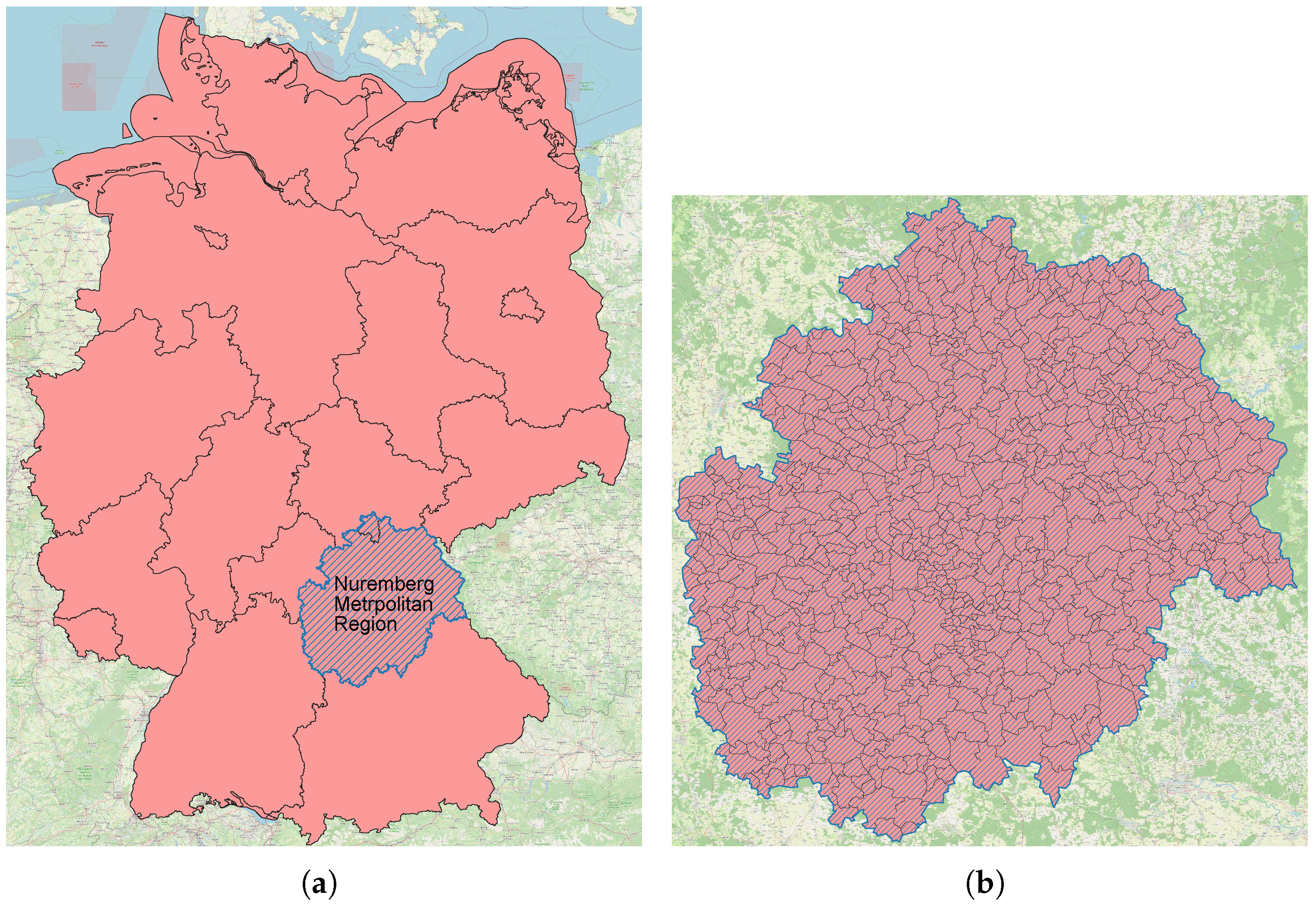
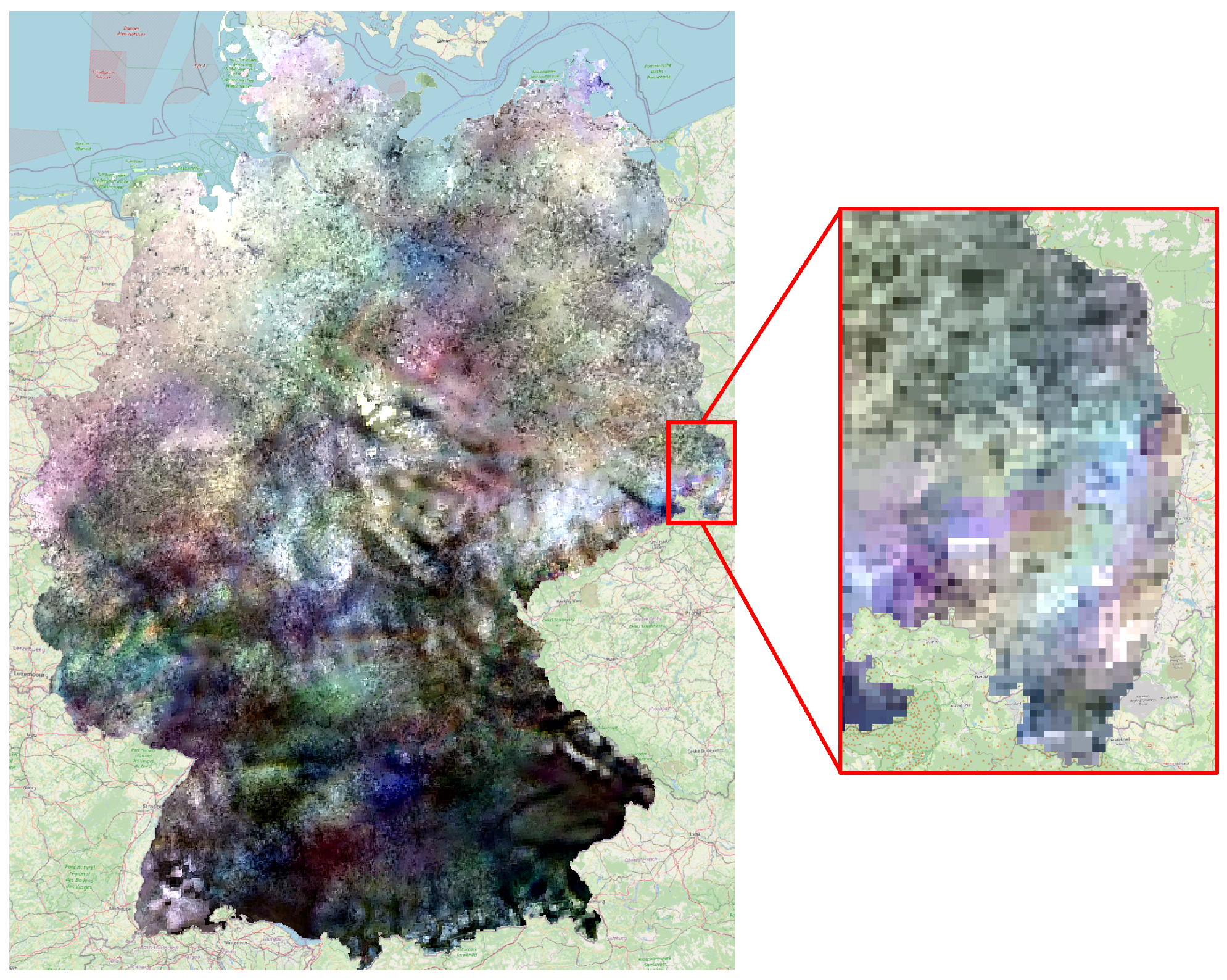
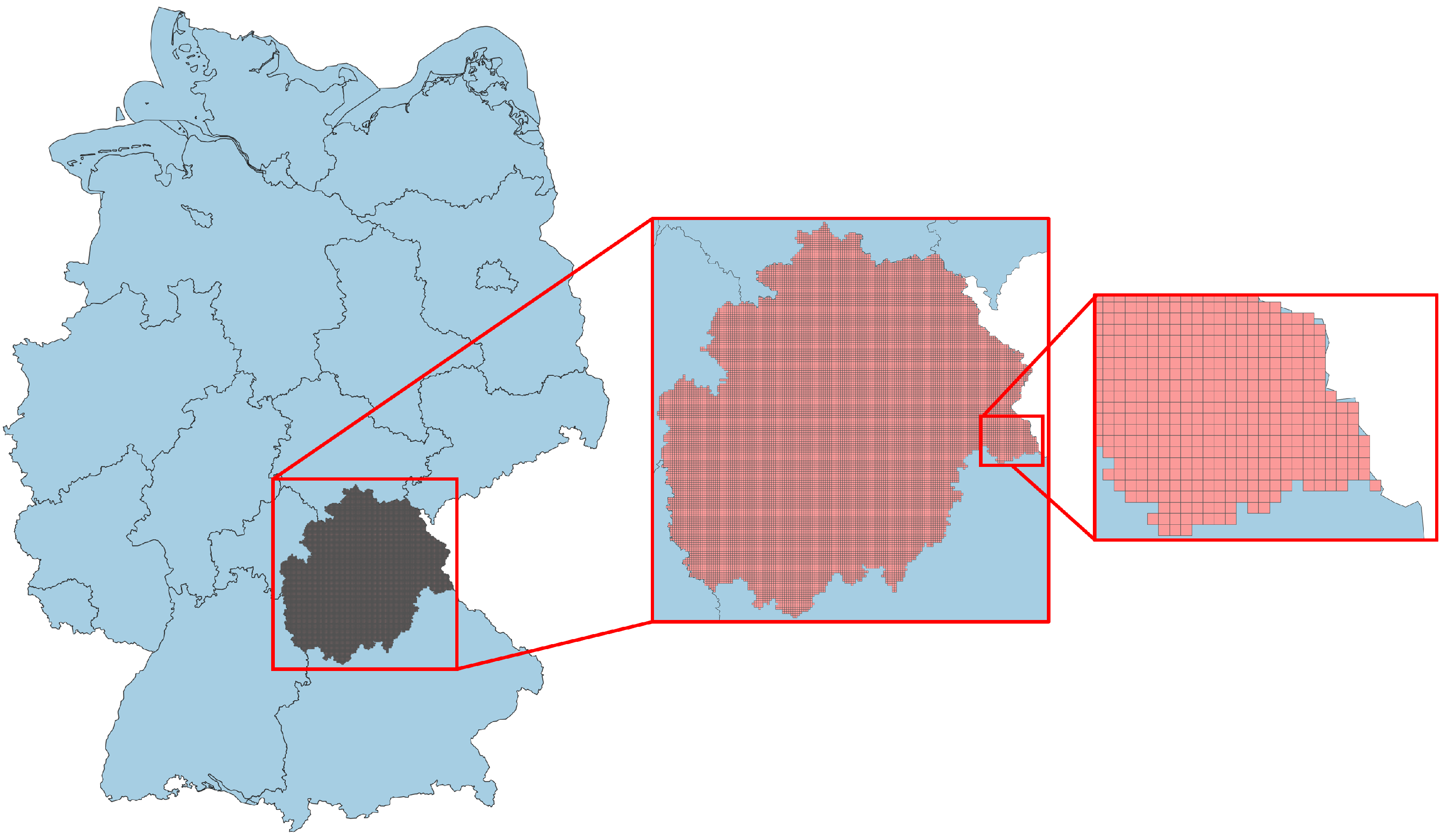
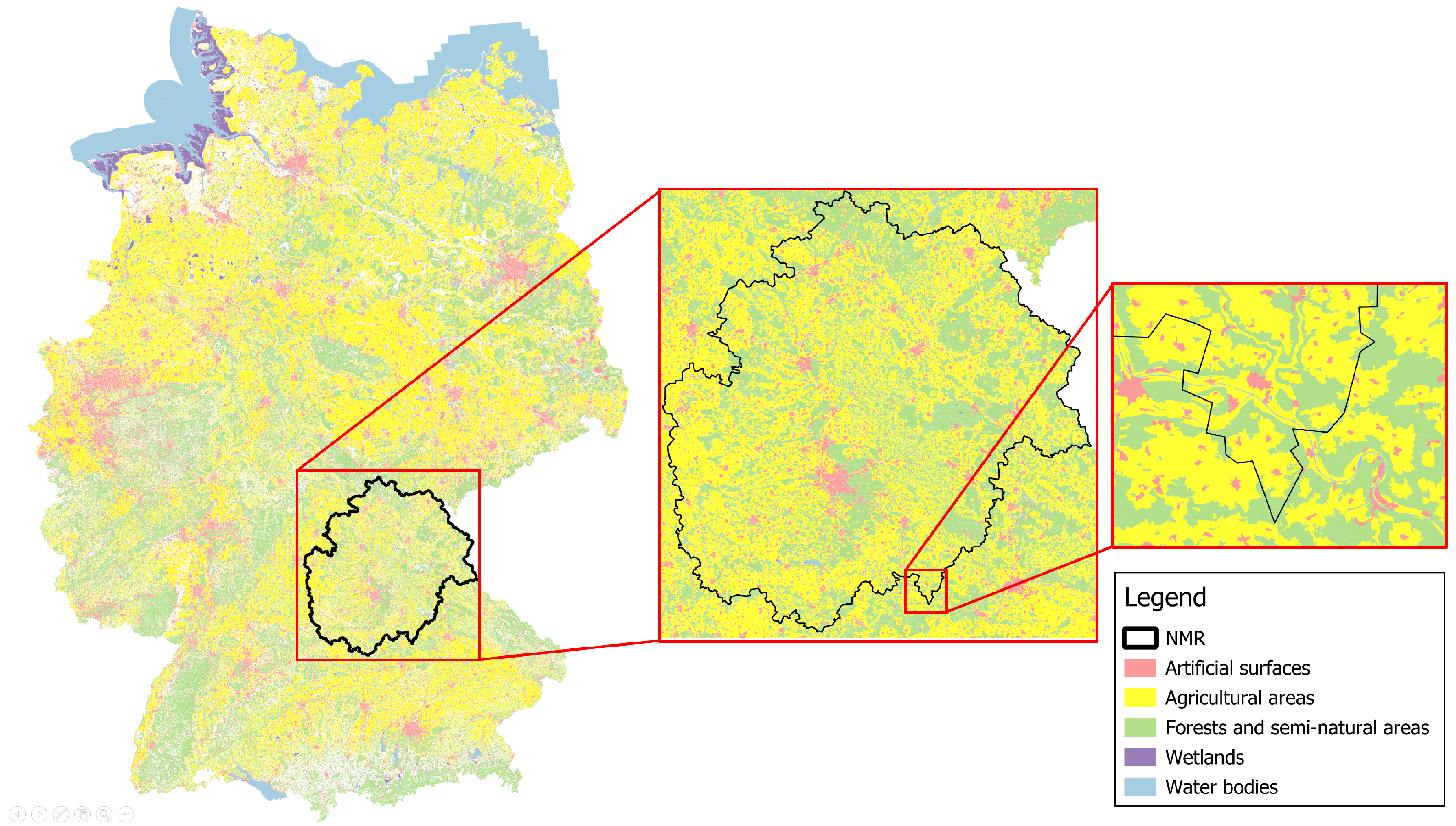
2.1. Visualization of the Model Region

Figure 1a illustrates the spatial context of the model region within Germany and delineates its territorial extent. For the purposes of the RES modeling framework, the NMR is divided into spatial units aligning with its administrative composition. This segmentation is based on publicly available geospatial data provided by the Federal Agency for Cartography and Geodesy [8], resulting in 676 distinct communities represented by the individual polygons shown in Figure 1b.

Each community is assigned a unique identifier, enabling unambiguous referencing and facilitating the integration of community-level data throughout the modeling process. The photovoltaic and wind power generation potentials are estimated separately for each community and subsequently spatially allocated to the region’s high-voltage substations. These generation profiles are superimposed with the sector-specific energy demands—stemming from the electricity, heat, and mobility sectors—to enable a subsequent load flow study. It should be noted, however, that the aforementioned simulation steps, including the load flow calculations lie beyond the scope of this publication and will not be discussed further herein.

2.2. PV Modeling Approach

The development of the PV modeling approach relies heavily on the availability and quality of data describing community-specific PV infrastructure. A key data source is the public installation registry maintained by the Federal Network Agency [9], which catalogs all generation facilities across Germany, including both privately and commercially operated PV systems. The aforementioned registry also includes system-specific community keys that enable the allocation of all PV systems to their respective municipalities, as they are congruent with the identifiers used to identify communities in the NMR. An evaluation of the register revealed several hundred thousand PV systems in the NMR, each of which was assigned to its corresponding community using the standardized identifiers.

Given the large number of installations and the limited availability of detailed open-access data, simulating each system individually was not feasible within the scope of the research project. Instead, an aggregation approach was developed to approximate PV feed-in behavior at the community level.

The aggregation method involves clustering the community-specific PV systems based on their technical specifications, including module orientation (azimuth angle) and module inclination (tilt angle), extracted from the installation registry. These groupings, which are based on the similarity of key technical parameters, are referred to as PV clusters throughout this study.

Several simulations were conducted to demonstrate the influence of system-specific parameters—particularly module orientation and inclination—on the feed-in behavior of PV systems. As illustrated in Figure 2, these characteristics significantly shape the temporal profile of PV power injection, particularly the daily feed-in curves. The results emphasize the necessity of accounting for such technical variations when modeling PV systems at scale. Accordingly, these findings substantiate the adopted clustering methodology, in which PV systems with comparable configurations are grouped together to form representative clusters. This approach enables a computationally efficient yet physically meaningful simulation of aggregated PV behavior at the community level.

Each PV cluster comprises systems with comparable technical characteristics, as identified through the clustering process. To represent the collective capacity of these systems, the aggregated nominal power $P_{nom,agg,Cl}$ of each PV cluster is calculated by summing the nominal powers of all individual PV systems assigned to that cluster—i.e., those matching its defining technical specifications. For a cluster Cl containing N systems, this yields

$$P_{nom,agg,Cl}=\sum _{i=1}^N{P}_{nom,Cl,i}.$$

(1)

The total nominal power $P_{nom,community}$ of all PV systems within a community is obtained by aggregating the cluster-level nominal powers $P_{nom,agg,Cl}$ across all of the community’s PV clusters.

$$P_{nom,community}=\sum _{i=1}^N{P}_{nom,agg,Cl,i}$$

(2)

The behavior of each PV cluster must be individually replicated, using its aggregated nominal power $P_{nom,agg,Cl}$ along with its technical specifications as the primary inputs. As a result, community-specific time series $P_{PV,Cl}\left(t\right)$ representative of each PV cluster’s power injection must be derived.

The total PV power injection of a community, $P_{PV,\mathrm{community}}\left(t\right)$, is obtained by aggregating the established time series $P_{PV,Cl}\left(t\right)$ of all its PV clusters. Accordingly, for a community comprising N PV clusters, the total PV power injection can be expressed as

$$P_{PV,community}\left(t\right)=\sum _{i=1}^N{P}_{PV,Cl,i}\left(t\right).$$

(3)

Numerical integration is used to determine the community’s corresponding energy quantity $E_{PV,community}$ resulting from the PV power injection $P_{PV,community}\left(t\right)$.

$$E_{PV,community}=\int P_{PV,community}\left(t\right)·dt$$

(4)

Furthermore, each community’s specific yield ${SY}_{community}$ is determined using the results provided by (2) and (4).

$${SY}_{community}={\displaystyle \frac{E_{PV,community}}{P_{nom,community}}}$$

(5)

Simulating these individual PV clusters greatly reduces the computational effort, while still effectively approximating the aggregated, community-specific PV feed-in behavior.

The preceding community-specific assessments can be extended to encompass the NMR as a whole by consolidating the individual communities:

$$P_{nom,NMR}=\sum _{i=1}^{676}{P}_{nom,community,i}$$

(6)

$$P_{PV,NMR}\left(t\right)=\sum _{i=1}^{676}{P}_{PV,community,i}\left(t\right)$$

(7)

$$E_{PV,NMR}=\sum _{i=1}^{676}{E}_{PV,community,i}$$

(8)

$${SY}_{NMR}={\displaystyle \frac{E_{PV,NMR}}{P_{nom,NMR}}}$$

(9)

Building on the previously described clustering methodology and nominal power aggregation, the next step involves generating time-resolved PV generation profiles for each community. While the technical configuration of PV systems significantly shapes their feed-in behavior, local meteorological conditions—particularly solar irradiance—are equally crucial for accurately modeling temporal variability. Therefore, the integration of location-specific weather data is essential to realistically capture the dynamics and variability of PV power injection within each cluster and, by extension, each community.

In the EMN_SIM framework, weather data is integrated using irradiance measurements provided by the weather stations of the Deutscher Wetterdienst (DWD) [10]. However, the spatial distribution of these stations is insufficient to allow for a direct, community-level meteorological characterization. To address this limitation, communities are grouped based on their geographic proximity to the nearest DWD weather station. Each community is thereby assigned a representative weather station, whose data serves as a proxy for the local irradiance conditions. This proximity-based clustering results in the weather station groups illustrated in Figure 3, where the locations of the reference stations are marked with star-shaped symbols.

The implementation of the proposed modeling approach involves simulating all combinations of azimuth and tilt angles—representing the defined PV clusters—under the irradiance conditions recorded at each weather station. This results in a set of standardized generation profiles that capture the influence of both system configuration and localized weather variability. Within the EMN_SIM framework, this process is performed using the Python-based library pvlib (0.11.0) [11] and is executed iteratively for each weather station and all PV clusters, as illustrated in Figure 4.

Following the initialization of weather data, an annual solar path is calculated for each weather station location. The PV systems are parameterized according to the technical specifications defining each PV cluster. Using this configuration, the system’s AC output power is simulated, accounting for both cluster-specific parameters and the site-specific solar trajectory. The resulting power curve is subsequently normalized to yield a standardized annual generation profile. Consistent component specifications are applied in all simulations—namely, a Canadian Solar CS6X-300M module (Canadian Solar, Guelph, ON, Canada) and an ABB MICRO-0.3-I-OUTD inverter (ABB, Zurich, Switzerland). Comprehensive tables of the site-specific irradiance data and the electrical characteristics of the reference module and inverter are provided in Appendix A.

Furthermore, an average degradation factor is considered when creating these annual profiles. This degradation is based on an average PV system age of 8 years (relying on the evaluation of the installation register) as well as an assumed annual degradation of 0.5% [12]. These annual profiles are established for all weather stations and the various tilt and azimuth angle specifications and saved as $P_{WS,AZ,Ti,std}$.

Using this approach, over 350 standardized annual profiles are generated in this manner, effectively serving as the base for modeling PV power injection within the NMR. Figure 5 illustrates one of these annual profiles, which was derived from measurement data collected at the weather station in Nuremberg, the largest city in the NMR.

These profiles are subsequently scaled using the corresponding aggregated nominal powers of the community-specific PV clusters, thus enabling a realistic representation of PV generation at the community level.

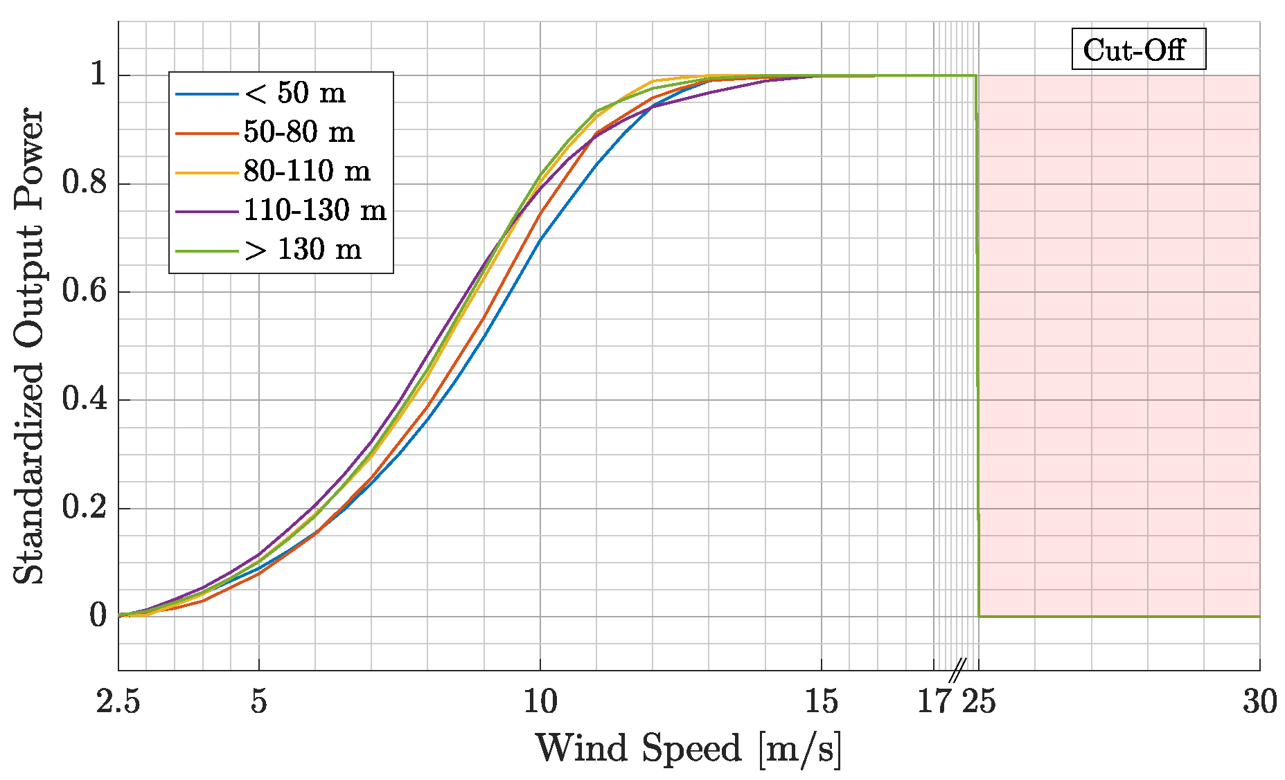
2.3. Wind Modeling Approach

This section outlines a methodology for deriving wind power generation profiles at the community level. The goal is to spatially approximate the disaggregated feed-in patterns of installed wind turbines, reflecting their geographic distribution and technical characteristics, under incorporation of suitable meteorological wind datasets to accurately capture local weather conditions.

Initially, all wind turbines within the NMR are identified and assigned to their respective communities, mirroring the approach used for PV systems. The turbines’ technical data is sourced from the same installation register maintained by the Federal Network Agency [9]. In addition, the registry stipulates georeferencing for generation units with capacities exceeding 100 $\mathrm{k}$$\mathrm{W}$, a threshold that encompasses the vast majority of wind turbines, thereby ensuring that most installations can be spatially identified with high accuracy. As a result, all wind turbines within the NMR can be visualized using a geographic information system (GIS), as shown in Figure 6.

This representation allows the data to be efficiently processed and filtered, making it possible to accurately identify which wind turbines are located within each community’s boundaries. The result is a detailed list of all communities with wind turbines, along with their technical characteristics—forming a solid foundation for modeling wind power generation at the community level within the NMR.

The proposed modeling approach simulates wind-dependent power generation for individual turbines based on a combination of technical and meteorological parameters. Central to this method are two key inputs: the wind speed at the turbine’s hub height and the corresponding turbine-specific power curve. Together, these inputs allow for the estimation of power output by linking local wind conditions to the turbine’s performance characteristics derived from manufacturer technical specifications.

The incorporation of realistic wind data greatly enhances the accuracy of the modeling approach. A straightforward and practical approach of implementing the model is through the direct integration of locally measured wind speed data, e.g., as provided by DWD weather stations [13]. However, wind speeds in Germany exhibit substantial spatial variability, as illustrated by the wind speed maps published by the Bavarian State Ministry [14], which highlight pronounced variation in both average wind speed and expected energy yield (see Figure 7).

Given the previously noted high spatial variability of wind conditions, using wind data with fine spatial resolution is essential for improving modeling accuracy. Unfortunately, direct measurements from DWD weather stations are unsuitable because of their relatively sparse geographic coverage. This study aims to circumvent the limitations of sparse station data by utilizing statistically derived wind raster data, which provides wind speed estimates at a substantially higher spatial resolution.

The raster data used in this study, referred to as HOSTRADA, is published monthly by the DWD and is openly accessible [15]. HOSTRADA is generated through the interpolation of DWD weather station data for most meteorological parameters, combined with satellite and climate model inputs to produce an internally consistent dataset [16]. This raster provides a wide range of meteorological variables, including wind speed (at a height of 10 m) across Germany, with each raster cell covering an area of 1 km by 1 km. Given the total surface area of Germany, this corresponds to approximately 360,000 grid cells, each represented by a pixel in Figure 8. For each cell, localized wind speed time series with an hourly resolution are available, enabling the detailed spatial and temporal modeling of wind conditions relevant to proposed approach.

A dedicated Python (3.10) script was implemented to restrict the scope of the HOSTRADA raster dataset to the region being modeled. As such, the script undertakes a filtering process by identifying and extracting only those cells whose centroids fall within the boundaries of the NMR. These boundaries are derived through the contiguous aggregation of NMR counties, based on geodata provided by [8]. The final result is the wind raster dataset for the year 2023 shown in Figure 9, representing the NMR region. Each grid cell, represented by the red squares, contains a time series of 8760 hourly wind speed values, annually capturing localized wind conditions.

The wind turbine locations shown in Figure 6 are matched to the raster cells in the HOSTRADA dataset, representative of their respective coordinates. This linkage provides the localized weather data crucial for accurately modeling each turbine’s power generation.

In a subsequent step, the raster data, representative of the wind speeds ($v_1$) at a height of 10 $\mathrm{m}$ ($h_1$), must be adjusted to reflect wind speeds ($v_2$) at the turbines’ hub heights ($h_2$). The conversion is based on the approaches published by Quaschning in [17]:

$${\displaystyle \frac{v_2}{v_1}}={\left({\displaystyle \frac{h_2}{h_1}}\right)}^a\to v_2=v_1·{\left({\displaystyle \frac{h_2}{h_1}}\right)}^a,$$

(10)

$$a={\displaystyle \frac{1}{ln\frac{z}{z_0}}},$$

(11)

$$z=\sqrt{h_1·h_2}.$$

(12)

The $z_0$ value is terrain-dependent and is provided as a table by [17], according to [18]. In this study, the site-specific $z_0$ parameter for wind turbines is determined based on the land use classification of the area where the turbine is located. To achieve this, the CORINE Land Cover dataset (CLC5) [19] is used to classify the terrain specific to each turbine. The CLC5 dataset systematically classifies land use and land cover in Germany into specific categories, as showcased in Figure 10.

The wind turbines illustrated in Figure 6 are cross-referenced to the polygons contained in CLC5 (shown in Figure 10), As a result, each turbine’s $z_0$ parameter is specified using the corresponding area’s land usage classification (CLC ID), according to the mapping table shown in

Table 1. Mapping table used for determining z0 in relation to the CLC ID.

CLC ID	CLC-Class Name	${\mathit{z}}_0$ Class	${\mathit{z}}_0$
112	Discontinuous urban fabric	Regularly covered with obstacles (forests, villages, suburbs)	1
121	Industrial or commercial units and public facilities	Regularly covered with obstacles (forests, villages, suburbs)	1
211	Non-irrigated arable land	Agricultural areas with low vegetation cover	0.1
231	Pastures, meadows and other permanent grasslands under agricultural use	Open flat terrain, grasslands	0.03
311	Broad-leaved forest	Regularly covered with obstacles (forests, villages, suburbs)	1
312	Coniferous forest	Regularly covered with obstacles (forests, villages, suburbs)	1
313	Mixed forest	Regularly covered with obstacles (forests, villages, suburbs)	1
324	Transitional woodland/shrub	Park landscapes with bushes and trees	0.5

. Thus, (10) and (11) offer straightforward formulas for converting each grid cell’s ground-level wind speeds to hub-height wind speeds that can be easily integrated into the simulation model’s framework.

System-specific power curves are utilized to model the power output of each unit, thus considering each system’s technical parameters as well as factoring in local wind speeds. A wind turbine’s power curve is a graph that shows the turbine’s relationship between wind speed and its electrical power output. It illustrates how much power a turbine can generate at different wind speeds, typically in the range from cut-in wind speed to cut-out wind speed [20]. The NMR contains approx. 680 wind turbines stemming from different manufacturers with a large variety of turbine types. Individually sourcing the power curve for each unique turbine type is not feasible. Instead, the wind generators are categorized based on their hub height, and a single, shared power curve is used to represent all units within each height category. Individual height categories are defined for the following hub heights: <50 m, 50–80 m, 80–110 m, 110–130 m and >130 m.

Each height-specific power curve is derived by averaging and standardizing the power curves of the most common wind turbine types within that height cluster. These representative turbine types are listed in

Table 2. Height-specific wind turbines types used for categorization.

Height [m]	Turbine Types
<50	E40, LW52/750
50–80	E40, D4, E53, V47
80–110	E82, V90, MD77, NM82
110–130	E70, V90, N117
<130	E82, N117, V112, E101

, and the resulting averaged, standardized power curves are shown in Figure 11. The original power curve data is sourced from [21,22].

All of the power curves shown in Figure 11 are saved within the simulation’s framework in the form of a look-up table. This enables the corresponding standardized power value $P_{Std}\left(t\right)$ to be determined for a given wind speed $v\left(t\right)$.

$$P_{Std}\left(t\right)=P_{Std}\left\{v\left(t\right)\right\}=LookUpTable\left\{v\left(t\right)\right\}$$

(13)

The feed-in power $P_{Turbine}\left(t\right)$ of each turbine is calculated by scaling the system’s nominal power $P_{Nom}$ with the standardized power value $P_{Std}\left(t\right)$.

$$P_{Turbine}\left(t\right)={P_{Nom}·P}_{Std}\left(t\right)$$

(14)

In summary, modeling each turbine’s output power is based on the procedure shown in Figure 12:

The community-specific wind power generation $P_{Wind,community}\left(t\right)$ is determined by aggregating the individual power shares $P_{Turbine}\left(t\right)$ of all turbines contained within the respective community. As such, the wind power generation $P_{Wind,community}\left(t\right)$ of a community with N wind turbines is given by

$$P_{Wind,community}\left(t\right)=\sum _{i=1}^N{P}_{Turbine,i}\left(t\right)$$

(15)

Numerical integration is used to determine the community’s corresponding energy quantity $E_{Wind,community}$ resulting from the wind power injection $P_{Wind,community}\left(t\right)$.

$$E_{Wind,community}=\int P_{Wind,community}\left(t\right)·dt$$

(16)

The preceding community-specific assessments can be extended to encompass the NMR as a whole by consolidating each of the NMR’s 676 individual communities:

$$P_{Wind,NMR}\left(t\right)=\sum _{i=1}^{676}{P}_{Wind,i}\left(t\right)$$

(17)

$$E_{Wind,NMR}=\sum _{i=1}^{676}{E}_{Wind,community,i}$$

(18)

3. Results and Discussion

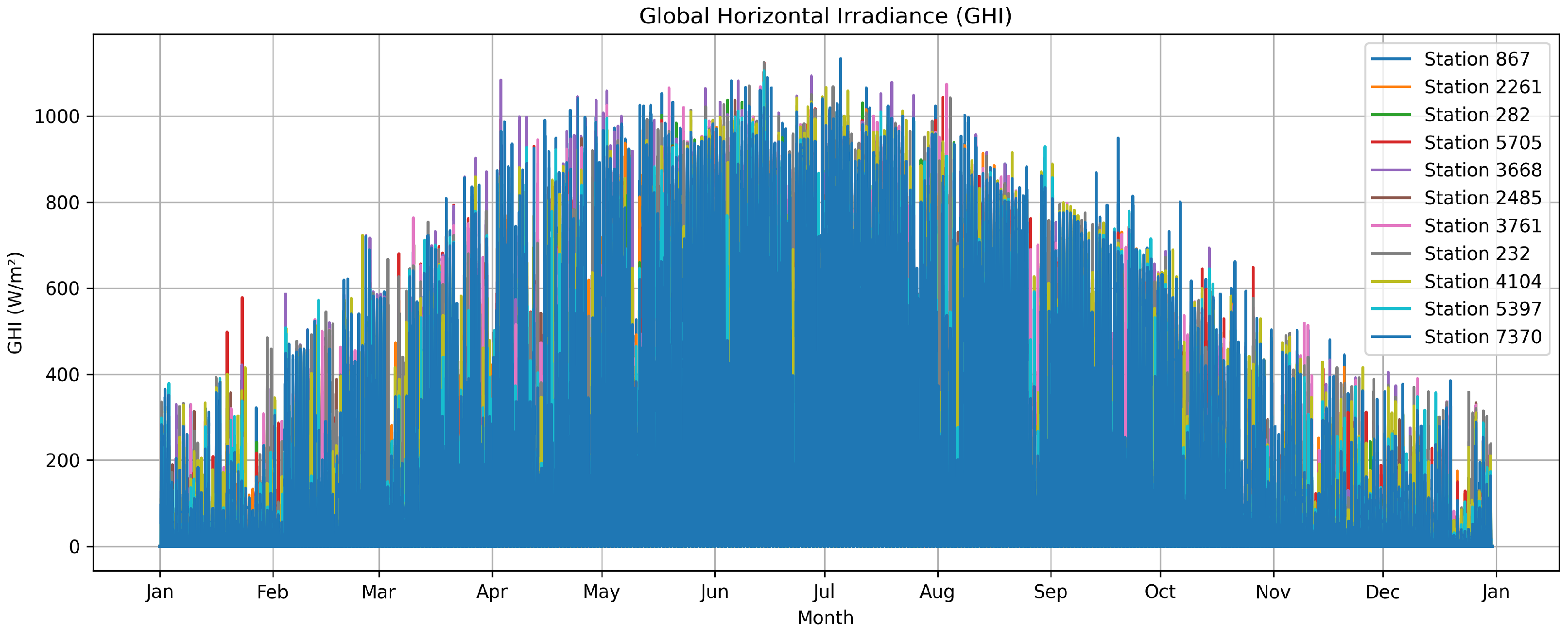
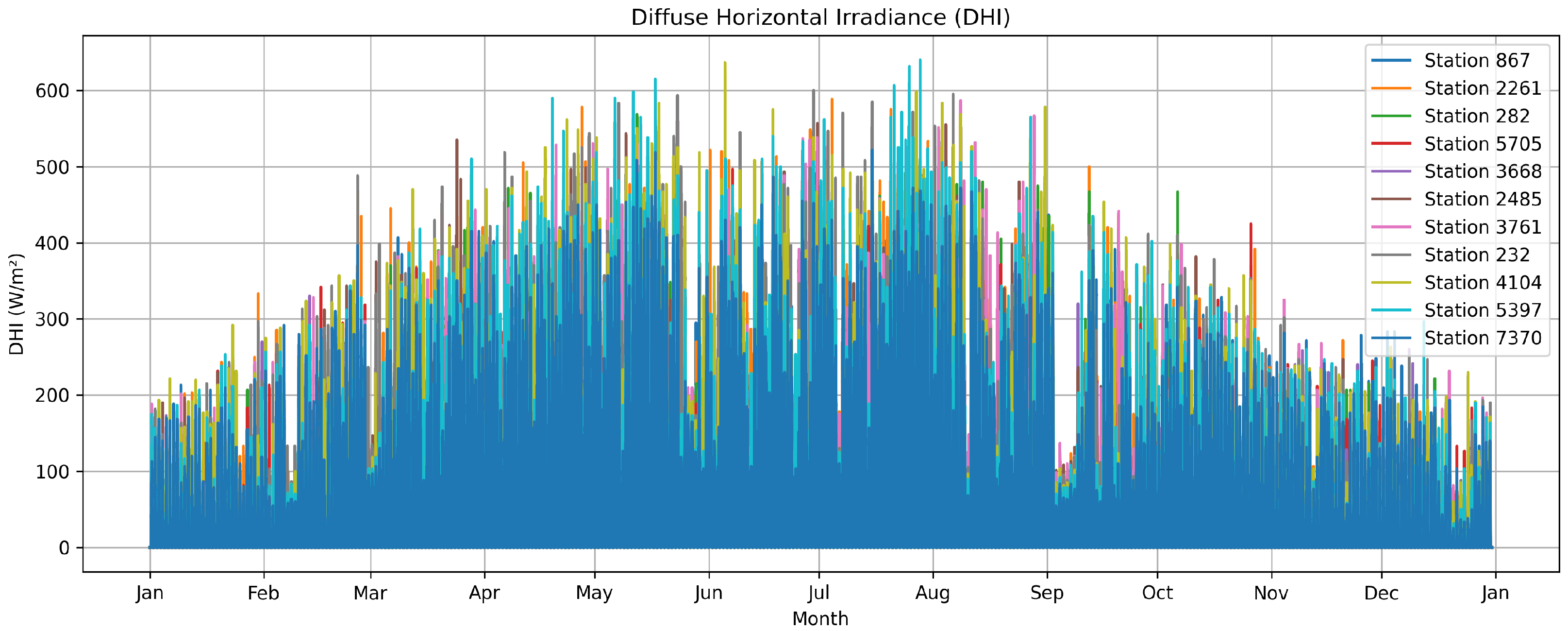
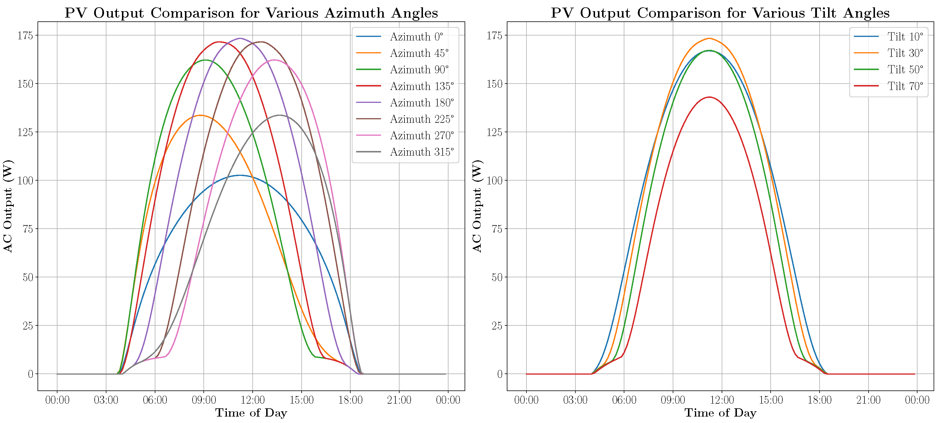
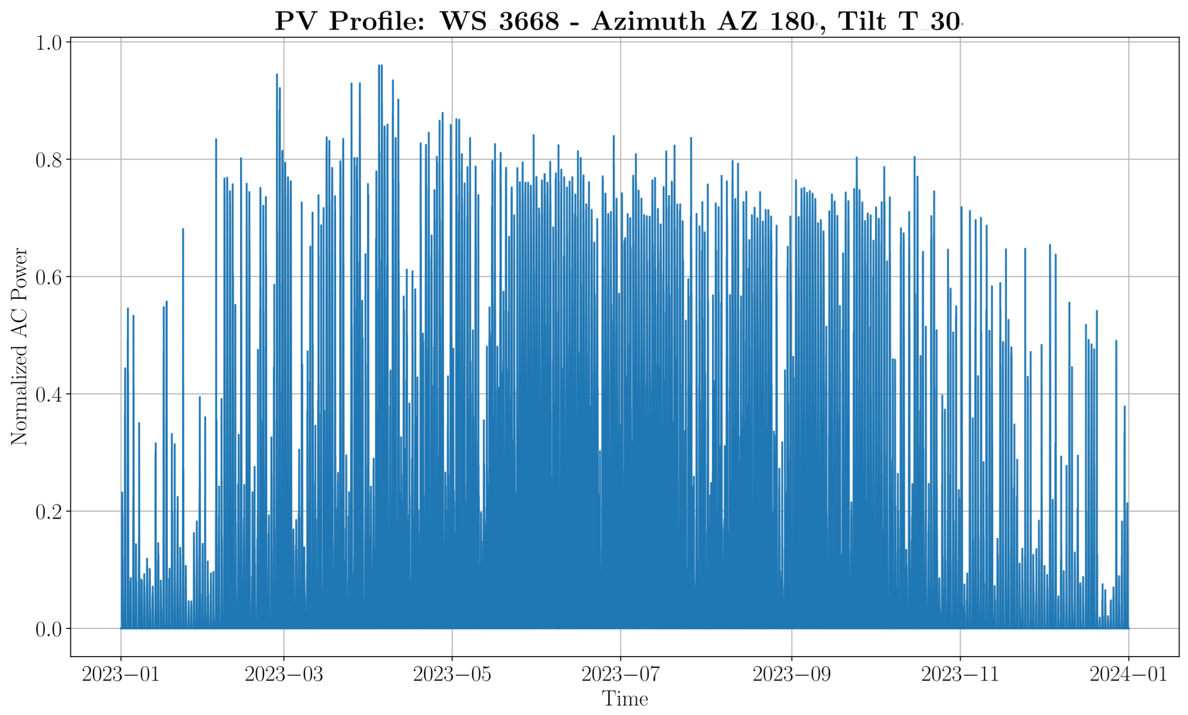
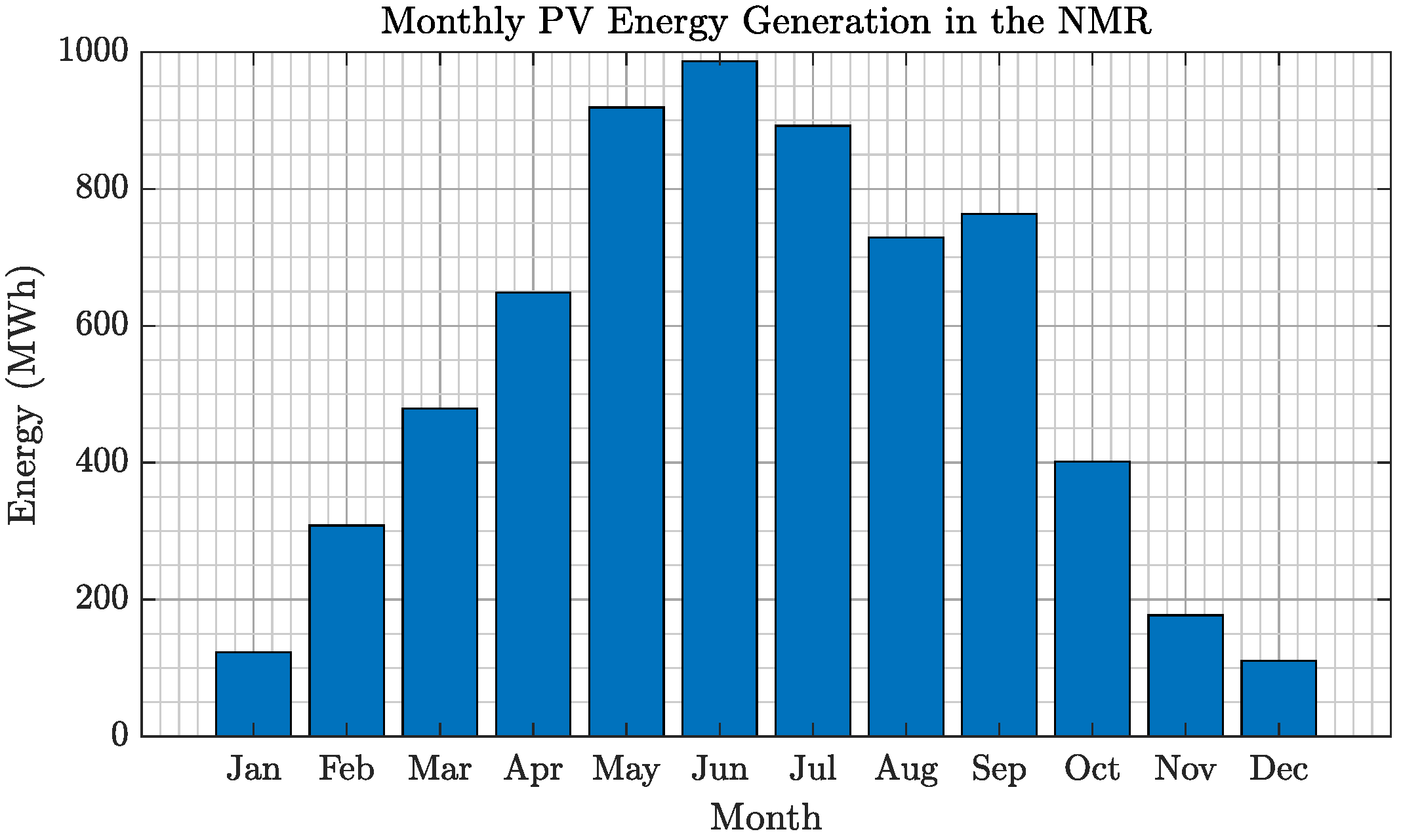
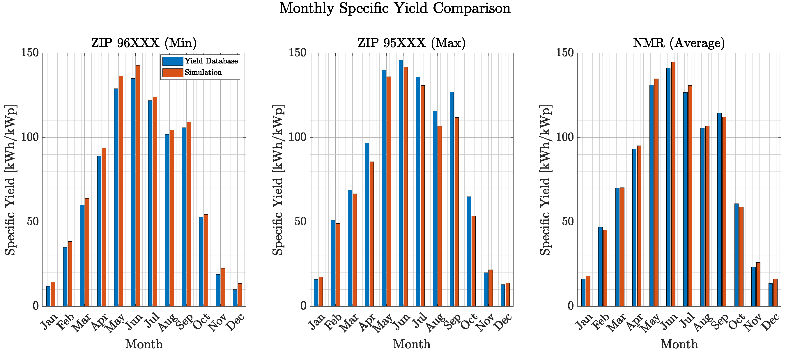
All results presented in this section are based on simulations conducted using the agent-based modeling software AnyLogic (8.8.6). The implemented model employs a class-based structure in which each community is represented as an agent. These agents are instantiated with parameters describing the PV clusters and wind turbines located within their boundaries. All necessary technical input data for these generation units—as well as meteorological inputs, preprocessed generation profiles, and other relevant parameters—are stored in the simulation’s directory and automatically loaded during model initialization. In addition, dedicated functions are implemented to calculate the community-specific renewable energy generation based on the modeling approaches outlined in Section 2. This structure supports a spatially resolved and scalable simulation of decentralized renewable energy generation across the NMR. The following results illustrate the resulting feed-in patterns and spatial dynamics captured by the model.

3.1. PV Simulation

During the simulation, each community’s PV cluster power injections $P_{PV,Cl}\left(t\right)$, are individually modeled by scaling their corresponding standardized profiles with their respective aggregated nominal power $P_{nom,agg,Cl}$. Consequently, the time series representing the $i^{th}$ cluster’s power injection $P_{PV,Cl,i}\left(t\right)$, is determined by referencing the matching standardized profile of the PV cluster $P_{WS,AZ,Ti,std}\left(t\right)$, accounting for the weather station (WS), azimuth (AZ), and tilt (Ti) parameters and scaling it by the cluster’s aggregated nominal power $P_{nom,Cl,i}$.

$$P_{PV,Cl,i}\left(t\right)=P_{WS,AZ,Ti,std}\left(t\right)·P_{nom,agg,Cl}$$

(19)

Finally, totaling the individual PV cluster’s power shares, as shown by (3), yields the desired total PV power injection of each community.

Using the proposed modeling framework in conjunction with Equations (4) and (5), the simulation quantifies the NMR’s photovoltaic output for the 2023 reference year. The model yields an annual energy production of 6538 GW h and an associated specific yield of 960 kWh/kWp, as depicted in Figure 13.

A direct validation of the simulation results at this level of regionalization—i.e., at the community or metropolitan region scale—remains challenging due to the absence of high-resolution reference measurements. Although comprehensive energy use studies for the metropolitan region exist, the most recent dataset dates back to 2019 [23], which does not correspond to the simulation’s reference year of 2023, limiting direct annual energy volume comparisons.

For a more direct evaluation of the simulation’s accuracy, a nationwide PV yield database [24] is used. This database contains recorded measurement data from approximately 20,000 PV systems across Germany, including specific yield data localized by German zip codes. The data is matched to the boundary conditions of the implemented simulation—namely, its geographic localization and the reference year 2023. By extracting the monthly specific yields for all zip codes within the NMR, this dataset provides a geographically consistent real-world baseline for comparison. This approach ensures that the simulated data are evaluated against real measurement data obtained under comparable conditions, thereby strengthening the validation.

Specifically, the comparison focuses on zip codes representative of the NMR region, ranging from 90XXX to 97XXX (German zip codes consist of five digits, and the first two digits often indicate the broader regional location. For example, codes starting with 90 to 97 typically refer to areas in northern Bavaria, including the Nuremberg Metropolitan Region). The comparison between the simulated and measured specific yields for these areas, summarized in

Table 3. Monthly specific yield comparison in the NMR (2023).

Zip/Month	Jan	Feb	Mar	Apr	May	Jun	Jul	Aug	Sep	Oct	Nov	Dec	Annual	Note
90XXX	17	52	73	93	130	143	124	101	115	62	26	16	953
91XXX	17	52	73	93	130	143	124	101	115	62	26	16	953
92XXX	19	46	70	89	128	137	129	108	114	66	27	13	947
95XXX	16	51	69	97	140	146	136	116	127	65	20	13	996	Max
96XXX	12	35	60	89	129	135	122	102	106	53	19	10	870	Min
97XXX	16	46	75	99	130	144	126	106	111	57	22	14	945
Zip Mean:	16.2	47.0	70.0	93.3	131.2	141.3	126.8	105.7	114.7	60.8	23.3	13.7	944.0
Simulation	18.1	45.3	70.3	95.2	134.9	144.9	131.0	107.0	112.1	58.9	26.0	16.2	960.0	Average

, highlights the model’s ability to realistically capture PV generation patterns within the NMR.

Figure 14 presents the simulated, averaged specific yields of the NMR in the form of a bar chart and compares them to the measurement-based reference values. Additionally, the comparison is extended by separately analyzing the region with the lowest specific yields (ZIP: 96XXX) and the region with the highest specific yields (ZIP: 95XXX), which are compared to the corresponding simulation values.

The comparison in Figure 14 indicates a strong correlation between the simulated specific yields and those derived from the measured data provided by the yield database. Although a direct validation of the simulation results at the community level was not implementable, the prior specific yield comparison is enough to reinforce the credibility of the proposed PV modeling approach.

Furthermore, a comparison of annual PV energy volumes illustrates the significant expansion of photovoltaic installations in the model region. In 2019, the annual energy volume was recorded at 3372 GW h according to [23], whereas the simulation results for 2023 reflect the growth realized since then.

An additional evaluation of the PV simulation results is conducted through comparison with regional yield data from recent literature. Hessen et al. [25] present specific yield data across various postal code areas in Germany for 2020. Within the NMR region, yields range from 894 kW h kW⁻¹ to 1142.3 kW h kW⁻¹, based on a standardized system configuration featuring a south-facing orientation and a 30° tilt angle. The specific yields calculated in this study fall within this range, confirming the plausibility of the proposed modeling approach.

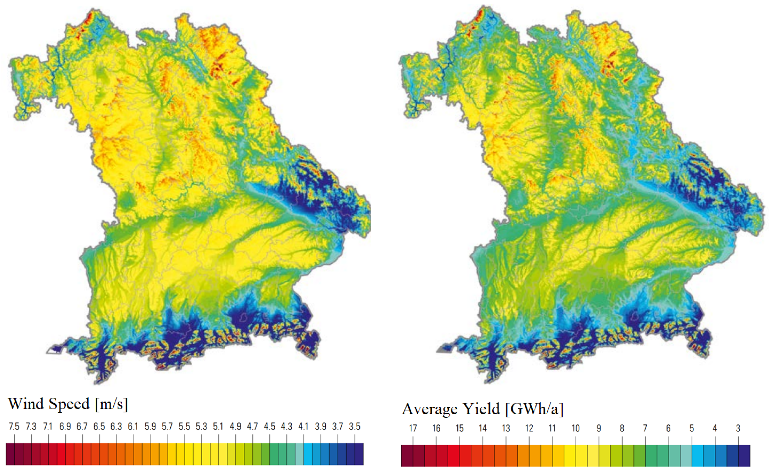
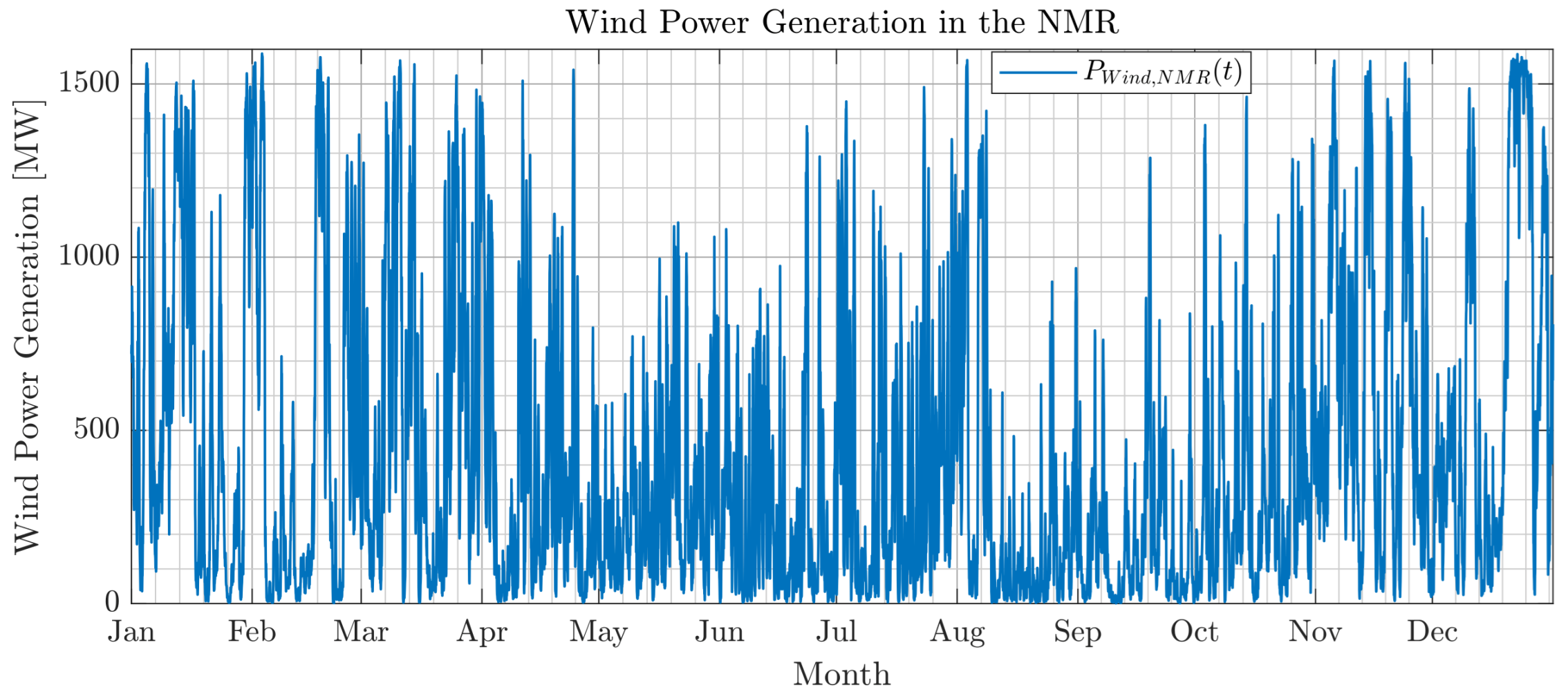
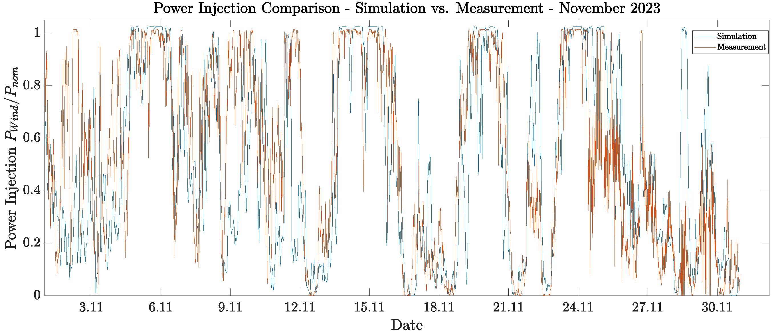
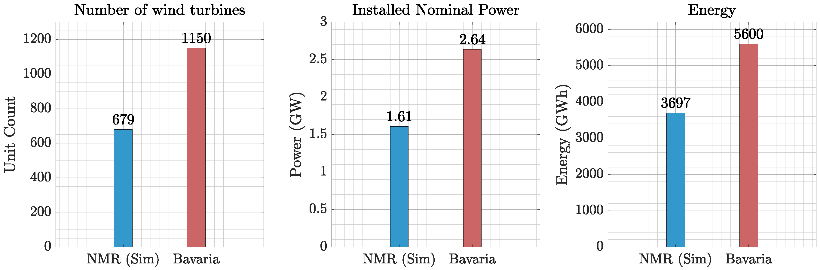
3.2. Wind Simulation

In contrast to the PV simulation, the modeling of wind power generation at the community level is based on the calculation of power outputs from individual wind turbines. Each turbine’s output is determined using its specific technical parameters and localized wind speed data. The resulting power injections are subsequently aggregated for each community, yielding a spatially resolved representation of wind energy feed-in across the NMR. Accordingly, the wind power feed-in and annual energy output for the NMR, shown in Figure 15 and Figure 16, are calculated using (17) and (18), respectively. The simulation indicates that wind turbines in the NMR fed approximately 3697 GW h of electrical energy into the grid in 2023, with a cumulative peak load exceeding 1500 MW.

The comprehensive and holistic validation of simulation results at the turbine level is constrained by the limited availability of high-resolution, publicly accessible feed-in data encompassing the entire population of wind turbines within the NMR. However, to nevertheless evaluate the model’s accuracy, a comparison was performed using actual measurement data from two exemplary wind turbines within the NMR for which detailed monitoring data was available. These real-world datasets are spatially aligned with the corresponding turbine-specific simulations, thereby enabling a direct and location-specific comparison of measured and simulated power output.

Selecting an appropriate validation window presents a notable challenge, as real-world wind turbine operation is often affected by curtailments and external interventions—such as shutdowns for animal protection or grid congestion management—that are not modeled in the simulation. To ensure a fair and meaningful comparison, November 2023 was deliberately chosen as the validation window due to its minimal operational disturbances. This ensures that the comparison is based on representative, undisturbed operation, providing a meaningful assessment of the model’s ability to replicate turbine-level wind power generation under typical conditions (see Figure 17).

The comparison between the simulated and recorded power profiles exhibits a very good fit in several periods, while other sections show noticeable discrepancies. Despite these differences, a clear overall correlation between the measured and simulated curves is evident, demonstrating the model’s general capability to capture the temporal dynamics of wind power generation. The deviations are likely attributable to limitations in the quality and spatial resolution of the underlying wind resource data used for the simulation. Specifically, the meteorological wind data is derived from raster grids with relatively coarse spatial resolution, which may not fully capture localized wind variations influenced by terrain, obstacles, or microclimatic effects. For context, studies such as [14] employ raster data with much finer spatial resolution on the order of 10 × 10 m, allowing for a more precise representation of site-specific wind conditions. The use of coarser data in this study may thus introduce smoothing effects and reduce the accuracy of turbine-level power output simulations. Additionally, unmodeled factors such as short-term turbulence and turbine control strategies can also contribute to the observed discrepancies.

Building on the preceding power-based comparison—limited to individual turbines due to data constraints—an additional energy-based assessment is conducted to validate the simulation results at the broader regional scale of the NMR.

In Germany, municipalities and cities are obligated to publish energy use plans as strategic instruments to facilitate the implementation of energy transition measures. The most recent plan encompassing the NMR was published in 2019 [23] and includes an assessment of wind energy generation based on the reference year 2016. Despite this, a direct comparison between this assessment and the 2023 simulation results presented in this study is methodologically inappropriate due to substantial differences in the respective boundary conditions. Specifically, the extent of wind energy deployment has evolved considerably over this period, with notable increases in both the number of turbines and installed capacity. In addition, interannual meteorological variability—particularly fluctuations in wind speed and distribution—introduces further discrepancies that can significantly affect energy yield. These differences rule a direct comparison and confound any attempt to validate simulation outputs relying on the NMR energy use plan.

Given the limitations associated with the NMR’s latest energy use plan, and the fact that a substantial portion of the NMR lies within Bavarian territory, the present study draws on official Bavarian energy statistics from 2023 to provide a more appropriate reference for validation. These statistics offer regionally representative and contemporaneous benchmarks, encompassing key indicators such as the number of installed wind turbines [26], total nominal capacity [27], and annual wind energy generation [28]. Compared to the outdated 2016 reference, these 2023 data reflect current deployment levels and prevailing meteorological conditions, thereby enabling a more robust and meaningful assessment of the consistency between simulated and observed regional wind energy trends (see Figure 18).

The comparable relationship between the number of turbines and their total installed nominal capacity in both the NMR and Bavaria indicates a similar average system size. This similarity is expected, given that the NMR is geographically embedded within Bavarian territory, and it supports the assumption that wind infrastructure characteristics are broadly comparable across both regions. Based on this premise, an energy-based validation of the simulation results is conducted by comparing the average full load hours (FLH) of wind turbines in the NMR and in Bavaria, as defined in Equations (20) and (21).

$${FLH}_{NMR}={\displaystyle \frac{E_{NMR}}{P_{nom,NMR}}}={\displaystyle \frac{3697\mathrm{G}\mathrm{W}\mathrm{h}}{1.61\mathrm{G}\mathrm{W}}}\approx 2296\mathrm{h}$$

(20)

$${FLH}_{Bavaria}={\displaystyle \frac{E_{Bayern}}{P_{nom,Bayern}}}={\displaystyle \frac{5600\mathrm{G}\mathrm{W}\mathrm{h}}{2.636\mathrm{G}\mathrm{W}}}\approx 2124\mathrm{h}$$

(21)

The previously calculated full load hours for the NMR and Bavaria are of comparable magnitude, supporting the validity of the simulation results at the regional scale. It is important to note, however, that the simulation does not account for curtailments resulting from factors such as grid congestion management. According to estimates by the Federal Network Agency, approximately 3.978 TW h of the total 118.7 TW h of electricity generated by German onshore wind turbines in 2023 was curtailed, representing roughly 3.4% of total potential production [29,30]. This unmodeled reduction may lead to a slight overestimation in the simulated energy yields.

$${FLH}_{NMR,adj}\approx {FLH}_{NMR}·\left(1-0.034\right)\approx 2218\mathrm{h}$$

(22)

Applying the estimated curtailment rate of 3.4% to the simulation results yields an adjusted average of approximately 2218 full load hours. This value aligns even more closely with the corresponding reference values for Bavaria. From an energy-based perspective, these findings further support the validity of the simulation results and reinforce their consistency with observed regional performance.

An additional evaluation of the wind power simulation results is performed by comparing the modeled full load hours with reported values from the recent literature. BWE [31] provides an analysis of onshore wind power plants in Germany for the year 2022. For wind installations in Bavaria, the reported average full load hours amount to approximately 2230 h/a. This value closely matches the simulation results obtained in the present study, confirming the plausibility of the proposed modeling approach for wind energy systems.

4. Conclusions

This publication proposes modeling approaches suitable for portraying the community-specific power injection originating from wind turbines and PV generators within a German metropolitan region. The research conducted within the context of this article was developed within the EMN_SIM research project, but is fundamentally applicable to any metropolitan region in Germany. Both the PV and wind modeling methodologies are implemented using openly accessible datasets.

The proposed PV modeling approach enables simulating community-specific PV power injection through the use of cluster-based aggregation methods, while incorporating real weather data and reducing computational effort. The validation of the developed PV modeling approach is conducted by comparing key system parameters, particularly the specific yield. As such, the regionally simulated specific yields are compared to those of real PV systems (measurement-based). Overall, the simulated specific yields closely align with the recorded data, thereby reinforcing the validity of the proposed approach from an energetic perspective.

The community-specific wind modeling approach is implemented on a per-plant basis, where system-specific parameters (e.g., wind power curves), environmental influences (e.g., land use), and the wind’s meteorological influence are accounted for by integrating real raster wind data. A validation of the simulation results is conducted from both energetic and power perspectives, thus ensuring a comprehensive assessment of the simulation. A power-based evaluation reveals a noticeable correlation between the simulation and measured reference values for two exemplary wind turbines. However, an exact match is not observed, presumably due to the limited resolution of the raster wind data. Nevertheless, from an energetic perspective, the simulation provides comparable average full-load hours for 2023 in relation to the Bavarian reference values.

The high-resolution, community-level generation profiles developed in this study provide a valuable foundation for policymakers seeking to design targeted renewable energy support schemes and grid planning strategies. By identifying spatial and temporal patterns in PV and wind generation, the results can inform investment in local infrastructure, such as storage systems or grid upgrades, and guide policy instruments to areas with the highest impact. These insights support more efficient allocation of resources and help municipalities advance decarbonization goals while maintaining grid reliability.

However, a key limitation lies in the restricted availability of high-resolution, measurement-based validation data for both wind and PV models. The wind model validation was limited to two reference turbines, while the PV validation relied on aggregated national data rather than region-specific measurements. This limits the statistical robustness and precision of the validation results. To address this, future work will actively seek additional real-world validation data from local utilities, SCADA systems, and open-data initiatives to enhance model calibration and uncertainty assessment.

As a next step, the validated generation profiles will be combined with sector-specific energy demand profiles for electricity, heat, and mobility. This integration will enable detailed load flow simulations to evaluate grid stability, hosting capacity, and flexibility options, such as demand response and storage. These simulations are beyond the scope of this publication but constitute a central direction within the EMN_SIM project.

References

1. Iweh, C.D.; Gyamfi, S.; Tanyi, E.; Effah-Donyina, E. Distributed Generation and Renewable Energy Integration into the Grid: Prerequisites, Push Factors, Practical Options, Issues and Merits. Energies 2021, 14, 5375. [Google Scholar] [CrossRef]
2. Oyekale, J.; Petrollese, M.; Tola, V.; Cau, G. Impacts of Renewable Energy Resources on Effectiveness of Grid-Integrated Systems: Succinct Review of Current Challenges and Potential Solution Strategies. Energies 2020, 13, 4856. [Google Scholar] [CrossRef]
3. Müller, S.; Möst, D.; Fichtner, W. A Spatially Resolved Model of the German Electricity Sector to Evaluate Energy Transition Pathways. Electr. Power Syst. Res. 2018, 164, 177–190. [Google Scholar] [CrossRef]
4. Sossan, F.; Bindner, H.; Marinopoulos, A.; Paolone, M. Probabilistic Characterization of Power Flows in Distribution Networks with High Penetration of Renewable Energy Sources. IEEE Trans. Power Syst. 2017, 32, 3464–3474. [Google Scholar]
5. Eckardt, T.; Lutz, M.; Schierhorn, P.; Müller, U.P. Impacts of Decentralized Generation on Medium Voltage Grid Planning—A Meso-Scale GIS-Based Assessment. Appl. Energy 2021, 282, 116098. [Google Scholar] [CrossRef]
6. Saha, T.K.; Nouri, H.; Pal, B.C. Impact of High Penetration of Renewable Energy Sources on Grid Frequency Behaviour: An Eigenvalue-Based Study. Int. J. Electr. Power Energy Syst. 2022, 141, 108701. [Google Scholar] [CrossRef]
7. Metropolregion Nuernberg: Klimapakt2030plus, Simulationsmodell. Available online: https://www.klimapakt2030plus.de/forschung/emn-sim (accessed on 9 January 2025).
8. Bundesamt für Kartographie und Geodäsie, Verwaltungsgebiete 1:5,000,000 (VG5000 01.01.), January 2024. Available online: https://gdz.bkg.bund.de/index.php/default/verwaltungsgebiete-1-5-000-000-stand-01-01-vg5000-01-01.html (accessed on 9 January 2025).
9. Bundesnetzagentur, Markstammdatenregister. Available online: https://www.marktstammdatenregister.de/MaStR/Datendownload (accessed on 9 January 2025).
10. Deutscher Wetterdienst, Solar Observations in Germany. Available online: https://opendata.dwd.de/climate_environment/CDC/observations_germany/climate/10_minutes/solar/historical/ (accessed on 9 January 2025).
11. Anderson, K.; Hansen, C.; Holmgren, W.; Jensen, A.; Mikofski, M.; Driesse, A. Pvlib python: 2023 project update. J. Open Source Softw. 2023, 8, 5994. [Google Scholar] [CrossRef]
12. Jordan, D.; Kurtz, S. Photovoltaic Degradation Rates—An Analytical Review. Prog. Photovoltaics: Res. Appl. 2013, 21, 12–29. [Google Scholar] [CrossRef]
13. Deutscher Wetterdienst, Stationskarte. Available online: https://www.dwd.de/DE/fachnutzer/landwirtschaft/appl/stationskarte/_node.html (accessed on 13 January 2025).
14. Bayerisches Staatsministerium für Wirtschaft, Landesentwicklung un Energie, Bayerischer Windatlas Potenzial der Windenergie in Bayern, February 2024. Available online: https://www.stmwi.bayern.de/fileadmin/user_upload/stmwi/publikationen/pdf/2024-02-01_Bayerischer_Windatlas_aktualisiert-2024.pdf (accessed on 13 January 2025).
15. Deutscher Wetterdienst, Climate Data Center—HOSTRADA Hourly Windspeeds. Available online: https://opendata.dwd.de/climate_environment/CDC/grids_germany/hourly/hostrada/wind_speed/ (accessed on 13 January 2025).
16. Deutscher Wetterdiesnst, HOSTRADA. Available online: https://www.dwd.de/DE/leistungen/uhi/info_methodic/01_hostrada.html (accessed on 13 January 2025).
17. Quaschning, V. Regenerative Energiesysteme: Technologie-Berechnung-Klimaschutz; Carl Hanser Verlag: München, Germany, 2013; p. 480. ISBN 978-3-446-47777-3. [Google Scholar]
18. Christoffer, J.; Ulbricht-Eissing, M. Die Bodennahen Windverhältnisse in der; Deutscher Wetterdienst: Offenbach, Germany, 1989. [Google Scholar]
19. Bundesamt für Kartographie und Geodäsie, CORINE Land Cober 5ha (CLC5-2018). Available online: https://gdz.bkg.bund.de/index.php/default/open-data/corine-land-cover-5-ha-stand-2018-clc5-2018.html (accessed on 13 January 2025).
20. Manwell, J.F.; McGowan, J.G.; Rogers, A.L. Wind Energy Explained: Theory, Design and Application, 2n ed.; John Wiley & Sons, Ltd.: Hoboken, NJ, USA, 2009. [Google Scholar]
21. Wind-Turbine-Models, Windkraftanlagen Datenbank. Available online: https://www.wind-turbine-models.com/turbines (accessed on 13 January 2025).
22. The Wind Power—Wind Energy Market Intelligence, E40/600. Available online: https://www.thewindpower.net/turbine_de_173_enercon_e40-600.php (accessed on 13 January 2025).
23. Energieagentur Nordbayern, Energienutzungsplan Europäische Metropolregion Nürnberg, August 2019. Available online: https://klimaschutz.metropolregionnuernberg.de/fileadmin/media/mediathek-klimaschutz/downloads/studien/2019-10-Energienutzungsplan.pdf (accessed on 13 January 2025).
24. Solarenergie-Förderverein, Ertragsdatenbank für Solarstrom. Available online: https://ertragsdatenbank.de/auswertung/region.html?j=2023&r=9&a=kurz (accessed on 13 January 2025).
25. Heesen, H. Photovoltaik-Ertragsstudie 2020: Regionale Erträge und Performance von PV-Anlagen in Deutschland; Umwelt-Campus Birkenfeld: Hoppstädten-Weiersbach, Germany, 2020; Available online: https://www.umwelt-campus.de/fileadmin/Umwelt-Campus/User/HteHeesen/research/pv/Ertragsstudie_2020.pdf (accessed on 15 June 2025).
26. Deutsche WindGuard, Anzahl der Windenergieanlagen in Bayern in den Jahren 2000 bis 2023, January 2024. Available online: https://de.statista.com/statistik/daten/studie/28315/umfrage/anzahl-der-windenergieanlagen-in-bayern-seit-1989/ (accessed on 14 January 2025).
27. Deutsche WindGuard, Kumulierte Nennleistung der Windenergieanlagen in Bayern in den Jahren 2000 bis 2023 (in Megawatt), January 2024. Available online: https://de.statista.com/statistik/daten/studie/28176/umfrage/installierte-leistung-durch-windenergie-in-bayern-seit-1989/ (accessed on 14 January 2025).
28. Bayerisches Staatsministerium für Wirtschaft, Landesentwicklung und Energie, Windenergie in Bayern. Available online: https://www.stmwi.bayern.de/energie/erneuerbare-energien/windenergie/#:~:text=Windenergieanlagen%20haben%20einen%20geringen%20Fl%C3%A4chenbedarf,2023%20betrug%205%2C6%20TWh%20 (accessed on 15 January 2025).
29. Bundesnetzagentur SMARD, Energiemarkt Aktuell–Netzengpassmangement im Jahr 2023, May 2024. Available online: https://www.smard.de/page/home/topic-article/444/213590 (accessed on 15 January 2025).
30. Bundesnetzagentur, Bundesnetzagentur Veröffentlicht Daten zum Strommarkt 2023, January 2024. Available online: https://www.bundesnetzagentur.de/SharedDocs/Pressemitteilungen/DE/2024/20240103_SMARD.html#:~:text=Insgesamt%20lag%20in%202023%20die,(100%2C6%20TWh%20) (accessed on 15 January 2025).
31. Bundesverband WindEnergie e.V. (BWE). Flächenpotenziale für die Windenergie an Land: Analyse und Ausblick; Bundesverband WindEnergie e.V. (BWE): Berlin, Germany, 2022; Available online: https://www.wind-energie.de/fileadmin/redaktion/dokumente/publikationen-oeffentlich/themen/01-mensch-und-umwelt/02-planung/20220920_BWE_Flaechenpotentiale_Windenergie_an_Land.pdf (accessed on 15 June 2025).
Figure 1. Visualization the NMR—serving as the model region in EMN_SIM. (a) Visualization of the NMR in the context of Germany; (b) visualization of solely the NMR.
Processes 13 02270 g001
Figure 2. Influence of azimuth and tilt angle on PV power injection (clear-sky model for Nuremberg, Germany; date: 1 June 2023).
Processes 13 02270 g002
Figure 3. Weather station-based community clustering.
Processes 13 02270 g003
Figure 4. Procedure for the generation of standardized annual PV profiles in pvlib.
Processes 13 02270 g004
Figure 5. Annual, standardized PV profile for the Nuremberg weather station (AZ = 180° S, Tilt = 30°, 2023).
Processes 13 02270 g005
Figure 6. Wind generators in the NMR.
Processes 13 02270 g006
Figure 7. Average wind speeds and corresponding yields in Bavaria at a height of 100 m.
Processes 13 02270 g007
Figure 8. HOSTRADA raster dataset covering all of Germany for the year 2023.
Processes 13 02270 g008
Figure 9. Subset of the HOSTRADA raster data filtered to the NMR, containing only raster cells within the model region.
Processes 13 02270 g009
Figure 10. CLC5: Depiction of land usage in Germany.
Processes 13 02270 g010
Figure 11. Averaged power curves for each cluster.
Processes 13 02270 g011
Figure 12. Procedure for calculating turbine-specific power output.
Processes 13 02270 g012
Figure 13. Monthly PV energy generation in the NMR (2023).
Processes 13 02270 g013
Figure 14. Bar chart showcasing the monthly specific yield comparison in the NMR (2023).
Processes 13 02270 g014
Figure 15. Total wind power generation P W i n d , N M R ( t ) in the NMR.
Processes 13 02270 g015
Figure 16. Monthly wind energy generation in the NMR.
Processes 13 02270 g016
Figure 17. Standardized power injection comparison (November 2023)—simulation vs. measurement.
Processes 13 02270 g017
Figure 18. Comparison of the number of wind turbines, installed wind capacity, and wind energy generated between the NMR and Bavaria in the year 2023.
Processes 13 02270 g018